

Abstract
A comprehensive mathematical model is proposed to study the transport phenomena in an Electrodialysis (ED) process employed to recover lithium hydroxide and sulfuric acid from the lithium sulphate solution derived from a recycling process of spent lithium-ion battery material. The model is developed based on the conservation equations of mass and ions, and considers electrolyte solutions consisting of mono- and multivalence ions. The concentration polarization at ion exchanged membranes (IEMs) and their adjacent diffusion boundary layers as a function of the applied current, inlet concentrations and flow rate are computed. Experimental data from a three-compartment ED cell are used for validation. A parametric study is performed to evaluate the impact of parameters on transmembrane fluxes of ion and water. It is revealed that increasing current leads to the enhancement of the transmembrane water and concentration polarization across IEMs. Feeding solutions consisting of smaller ions result in lower water transfer through IEMs. Raising the lithium concentration at the dilute channel increases the LiOH concentration due to reduced transmembrane water transfer. Using the uncertainty propagation method, it is found that current and counter-ion radius are the most influential parameters affecting the outlet concentration of concentrate channel and transmembrane water transfer.
Export citation and abstract BibTeX RIS
List of symbols

| Current density, A·m2 |

| Temperature, K |

| Channel width, m |

| Channel length, m |

| Channel height, m |

| Membrane thickness, m |

| Radius of species  m m |

| Hydrated radius of species  m m |

| Debye length, m |

| Diameter of species  m m |

| Membrane effective area, m2 |

| Outlet concentration of species  which exhaust from ED, mol. m−3 which exhaust from ED, mol. m−3
|

| Inlet concentration of species  which enter ED, mol·m−3 which enter ED, mol·m−3
|

| Concentration of species  in each tank, mol·m−3 in each tank, mol·m−3
|

| Average concentration of species  in membrane phase, mol·m−3 in membrane phase, mol·m−3
|

| The concentration of species  in the membrane side of a solution-membrane interface, mol·m−3 in the membrane side of a solution-membrane interface, mol·m−3
|

| The concentration of species  in the solution side of a solution-membrane interface, mol·m−3 in the solution side of a solution-membrane interface, mol·m−3
|

| Average concentration of species  in bulk solution, mol·m−3 in bulk solution, mol·m−3
|

| Concentration difference of species  across the IEM, mol·m−3 across the IEM, mol·m−3
|

| The diffusion coefficient of species  m2·s−1 m2·s−1
|

| Inlet velocity of solution entering ED, m·s−1 |

| Outlet velocity of solution exhausting from ED, m·s−1 |

| Transmembrane water velocity, m·s−1 |

| Solution volume in each tank, m3 |

| Volume of solution entering ED at the nth time step, m3 |

| Volume of solution discharged from ED at the nth time step, m3 |

| Transmembrane flux of species  mol. m−2·s−1 mol. m−2·s−1
|

| Transmembrane flux of water, m3·s−1 |

| Thickness of double layer, m |

| Wet weight of membrane, kg·m2 |

| Dry weight of membrane, kg·m2 |

| Maximum cycle number, 
|

| Total operation time of the batch-configuration ED, s |

| Resident time of solutions in the ED, s |

| Transport number of cations in membrane, 
|

| Transport number of anions in membrane, 
|

| The valence of species 
|

| Faraday's constant, 96485.33 A·s·mol−1 |

| Surface charge of membrane, C |

| The universal gas constant, 8.314 J. mol−1·K−1 |

| Volume fraction of liquid water in the IEM, 1 |

| water uptake, % |
| Greek symbols | |

| Surface charge density of membrane, C·m−2 |

| Zeta potential, V |

| Thickness of diffusion layer, m |

| Permittivity, F·m−1 or C2·J−1·m−1 |

| Relative permittivity, 
|

| Vacuum permittivity, F·m−1 or C2·J−1·m−1 |

| Limiting ionic conductance of species  at 298 K, m2·Ω−1·mol−1 at 298 K, m2·Ω−1·mol−1
|

| Limiting ionic conductance of species  at the temperatures T, m2·Ω−1·mol−1 at the temperatures T, m2·Ω−1·mol−1
|

| Dynamic viscosity, kg·m−1·s−1 or Pa·s |

| Water density, kg·m−3 |

| Constant, s·m−2 |

| Constant, mol. A−1·m−2 |

| Membrane potential difference, V |
| Superscripts | |

| Membrane side of IEM-solution interfaces |

| Solution side of IEM-solution interfaces |

| Bulk solution |

| Number of time step |
| Subscripts | |

| Membrane phase |

| Inlet |

| Outlet |

| Cations |

| Anions |

| Lithium ions |

| Hydroxide ions |

| Hydrogen ions |

| Sulfate ions |

| External tanks |
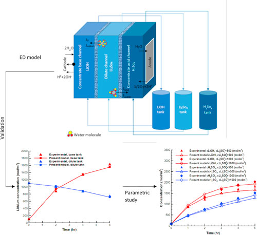
Electrodialysis (ED) is widely used in the desalination of brackish water and organic solutions, 1–4 producing salt, 5,6 demineralization of the boilers feed water, 7 and supplying the required water in food products. 8,9 Owing to the capability of ED in the separation of ionic species from other particles, such system is also used to extract metal ions and decrease the salinity of effluents and industrial waste streams, 10–12 as well as recovery of acid and base applications. 13,14 ED is an electrochemical separation process based on the transport of anions and cations within ion exchange membranes (IEMs) under the applied electrical field, which supplies the driving force of ion transport. Figure 1 illustrates the scheme of an electrodialysis cell, which consists of dilute and concentrate channels, anion and cation exchange membranes, as well as anode and cathode electrodes. Applying an electrical voltage between the electrodes leads to the transport of cations and anions toward the cathode, negatively charged electrode, and anode, positively charged electrode, respectively. Cations can pass through the negatively charged cation exchange membrane (CEM) and enter the concentrate base channel, while these ions are blocked to penetrate through the anion exchange membrane (AEM). Likewise, anions pass through the positively charged anion exchange membrane and arrive at the concentrate acid channel. As a result, the concentration of the dilute compartment decreases, while this amount increases at concentrate, namely base and acid channels. In addition, cations and anions that enter the base and acid channels react with the hydroxide and hydrogen ions, which are generated due to the water splitting at the surface of cathode and anode. Therefore, alkaline and acidic solutions are formed at the base and acid compartments, respectively.
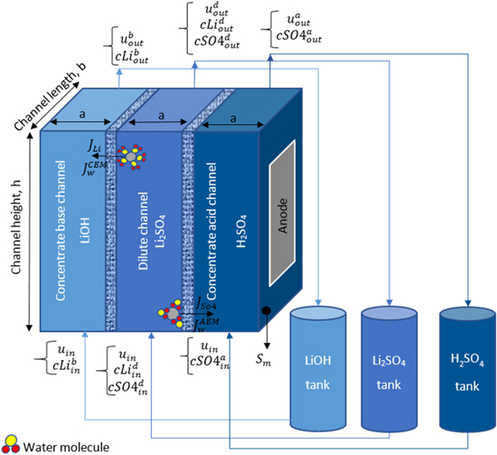
Figure 1. Schematic diagram of a batch-mode electrodialysis process for splitting Li2SO4.
Download figure:
Standard image High-resolution imageSeveral studies have been done to investigate EDs experimentally, e.g., 15,16 and some models have been proposed to predict their behaviour. 17–19 Previous studies mostly focused on the electrodialysis of NaCl solution or other solutions containing monovalent ions. 20 For instance, Mohammadi et al. 21 conducted a series of experiments and presented a mathematical model to evaluate the separation efficiency of EDs that operate at a constant voltage. This model proposed an empirical equation to predict the resistance of bulk solution as a function of temperature and concentration. Despite acceptable agreement between model results and experimental data, their model was not able to determine transmembrane water transfer. In an ED cell, due to the electro-osmotic water transport, i.e., movement of water molecules from dilute to concentrate compartments due to the passage of hydrated ions through IEMs, electrolyte concentration reduces at concentrate channels, while this amount increases at the dilute channel. Therefore, several investigations have been carried out to estimate the transmembrane water transfer and study its negative effects on ED performance. 22–24 Tanaka 17 presented a methodology to evaluate the flux of ions and water molecules within IEMs based on irreversible thermodynamics and the overall membrane characteristics, where empirical equations were used to estimate seawater electrodialysis. Using this methodology, ion and water transport equations, mass balance, and energy consumption relations, models for all single-pass, 25 feed and bleed, 26 as well as batch 27 configurations were developed. His model results showed good agreement with experimental data of NaCl electrodialysis, however, his models were unable to provide accurate results for solutions including multivalent ions.
Some studies have been carried out to investigate the concentration polarization of the diffusion boundary layers adjacent to IEMs. 28–30 To estimate counter- and co-ions concentrations at the solution side of a membrane-solution interface, Tanaka 28 proposed a correlation derived from the Nernst-Plank equation at the diffusion boundary layers adjacent to the IEM. Inspired by Tanaka's work for monovalent ions, the present study aims to develop an equation to determine concentration polarization at IEMs vicinity for 1–2 electrolyte solutions such as lithium sulphate (Li2SO4) and sulfuric acid (H2SO4).
In the present work, an ED test cell was set up to split Li2SO4 solution into LiOH and H2SO4, which are subsequently used in lithium-ion batteries recycling, which is a demanding and essential process due to the recovery of valuable and scarce metals such as lithium and environmental aspects. 31 The objective of the present study is to develop a comprehensive mathematical model to simulate single-pass and batch ED processes, such as this test cell. While electrodialysis of NaCl solution has been investigated in most previous mathematical models, the present model can be used for various solutions containing all mono and multi-valence ions. In this model, the fluxes of ions and water within the IEMs are computed as functions of concentration polarization at the IEM-solution interfaces. This model presents accurate results because of the independency of the model from empirical relations, consideration of the properties of membranes and mobile ions, as well as calculation of water flow through IEMs. A good agreement is observed between the experimental data and the present model results. Then, the effect of applied current, inlet concertation of the dilute channel, counter-ion size, membrane thickness and water volume fraction were investigated on the objective parameters, i.e., the water velocity through IEMs and concentrate channel's outlet concentration. Finally, uncertainty propagation was developed to study how these parameters affect the objective parameters and determine the influential ones.
The remainder of this paper is organized as follows.
Mathematical Modeling
A 1 + 1 dimensional (1 + 1D) mathematical model is developed in the present study to simulate the transport of species and ions in an electrodialysis process. Operation of the ED cell at constant-current for both single-pass and batch configurations are considered. In the batch configuration, all solutions are recirculated until certain desired concentrations are reached, as displayed in Fig. 1. The following assumptions are made to simplify the analysis:
- 1.Steady-state operation and laminar flow for all compartments.
- 2.Applied electric current is kept constant during the ED operation.
- 3.Temperature during the ED operation is constant.
- 4.The effect of pressure on ion transport, water velocity, and Donnan equilibrium approach is neglected.
- 5.The flux of co-ions through IEMs is zero; only counter-ions are allowed to penetrate through the IEMs.
Detailed derivations of the governing equations and specification of boundary conditions are presented in the following sections.
Conservation equations
The ions concentrations and velocity of the electrolyte solutions vary along the channels due to the fluxes of ions and water through the IEMs, which can be determined using material balance relations. Due to the transfer of ions and water molecules from the dilute channel to the concentrate channels, the concentration and velocity of the solution increase at the concentrate channels, while these quantities decrease in the dilute channel downstream. Therefore, the mass conservation equation for the solution and ions are presented in Eqs. 1 and 2, respectively, for all compartments as: 32

where  and
and  shown in Fig. 1, are the width, and length of channels, respectively,
 and
and  are the transmembrane water flux through IEMs, outlet and inlet velocities, respectively. Transmembrane water flux is written as
  and
and  for the anode and cathode channels, respectively. For the dilute channel,
  consists of the flux of water molecules moving through both anion and cation exchange membranes, i.e.,
The relationship between species flux across the membrane direction and net flow through each compartment can be expressed as:

with

where  and
and  are the membrane surface area and channels height,
  is the flux of species
  through an IEM,
  and
and  are the concentration of specie
  at the inlet and outlet of channels, respectively.
Species transport through IEMs
According to Eqs. 1 and 2, in order to find the outlet velocities and outlet concentration of lithium and sulphate ions, the flux of water and ions moving across IEMs must be determined first. Since the current remains constant during the ED operation and the flux of co-ions through IEMs is assumed to be zero, the flux of lithium and sulphate ions across IEMs are determined using Faraday's law as follows: 33

where  is Faraday's constant,
  is the valence of ion
  and
and  is current density defined as current divided per membrane area.
Water molecules tend to penetrate a membrane due to osmotic and electro-osmotic mechanisms. In the ED process, the osmotic water transport, i.e., the transfer of water molecules caused by the osmotic pressure or concentration difference across the membrane is negligible in comparison with the electro-osmotic phenomenon established by the transport of hydrated ions under the influence of an electrical potential gradient.
22,33–35
Hence, to determine the velocity of water molecules across a membrane, transmembrane water velocity, it is assumed that water molecules are dragged into IEMs by electro-osmotic force, which is a function of the applied electrical potential and the friction force that the ions encounter in the solution. Since these forces are equal in a steady-state condition, the water velocity through an IEM,  can be calculated as:
22,35
can be calculated as:
22,35

where  is the thickness of the membrane,
  is potential difference across the membrane,
  is dynamic viscosity,
  is the radius of counter-ion
  moving within the IEM,
22
and
moving within the IEM,
22
and  is the membrane surface charge density, i.e., the surface charge divided per the membrane area, that can be evaluated using the Helmholtz double-layer model:

where  is the surface charge. According to the Helmholtz model, the ions arranged at an IEM surface and the oppositely signed ions appealed to that membrane surface can be considered as capacitor plates at the distance of
  as depicted in Fig. 2(a).
35
Therefore, based on the capacity equation of capacitors,
36
Eq. 7 was proposed to evaluate membrane surface charge density.
35
as depicted in Fig. 2(a).
35
Therefore, based on the capacity equation of capacitors,
36
Eq. 7 was proposed to evaluate membrane surface charge density.
35

where  is called zeta potential representing the Helmholtz double-layer potential, as depicted in Fig. 2(b).
37
In the present study, the following relation is proposed to calculate zeta potential based on the surface charge and Eqs. 6 and 7.
is called zeta potential representing the Helmholtz double-layer potential, as depicted in Fig. 2(b).
37
In the present study, the following relation is proposed to calculate zeta potential based on the surface charge and Eqs. 6 and 7.

where  is the average concentration of species
  in a membrane, and
  is the diameter of counter-ion
  transferring through the membrane. In addition,
  is the permittivity of solvent and is defined as multiplying of the relative permittivity (dielectric constant),
  and the vacuum permittivity,
  as follows:
38
as follows:
38

where  is a constant value equal to 8.854 × 10⁻¹² F·m−1 and
  is calculated using Eq. 10 for dilute solutions:
21,39,40
is calculated using Eq. 10 for dilute solutions:
21,39,40

Finally, substituting Eq. 7 into Eq. 5 leads to:

and the flux of water is determined by:

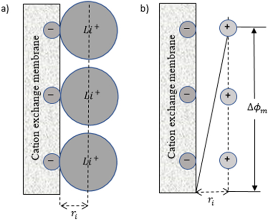
Figure 2. Schematic drawing illustrating: (a) the closest approach of lithium ions to the negatively fixed ions of the surface of a cation-exchange membrane, (b) the potential difference in the double layer according to the Helmholtz model.
Download figure:
Standard image High-resolution imageConcentration polarization at membrane-solution interfaces
In order to estimate the concentration of species at the solution adjacent to an IEM, Tanaka firstly developed Nernst-Planck equations for co- and counter-ions transferring at diffusion layer adjacent to the IEM.
28
Based on his methodology, Eq. 13 is developed to evaluate the concentration of ions at the solution side of an IEM-solution interface ( ) as a function of the bulk concentration, transmembrane water velocity, and diffusion coefficient of mobile ions in a single-salt solution:
28
) as a function of the bulk concentration, transmembrane water velocity, and diffusion coefficient of mobile ions in a single-salt solution:
28

where  is the thickness of diffusion layer, and superscript
  refers to the bulk solution. The following relations were introduced by Tanaka to define
  and
and  coefficients for monovalent salts, e.g., NaCl:
28
coefficients for monovalent salts, e.g., NaCl:
28


where subscripts  and − refer to cations and anions, respectively,
  is the transport numbers of ions in a membrane, and
  demonstrates the diffusion coefficient of ions at the solution. The present study proposes the equations listed in Table I to determine
  and
and  for divalent salts such as Li2SO4 as well as H2SO4 based on the development of Nernst-Plank equations at the diffusion boundary layers of IEMs vicinity.
Table I.
 and
and  coefficients for all solution-membrane interfaces.
| solution-membrane interface | Solution |
 s·m−2 s·m−2
|
 mol·A−1·m−2 mol·A−1·m−2
|
|---|---|---|---|
| Base channel-CEM |

|

|

|
| Dilute channel-CEM |

|

|

|
| Dilute channel-AEM |

|

|

|
| Acid channel-AEM |

|

|

|
It is noted that according to the assumption of zero co-ions flux through the IEM, the transport number of co-ions through IEMs, i.e., sulphate and lithium ions through cation- and anion-exchange membrane, respectively, is considered zero. In addition, water dissociation, i.e., H+ and OH− production, occurs in the over-limiting current densities. Therefore, the transport number of H+ and OH− species at the concentrate interfaces of IEMs would be negligible when the applied current density is lower than the limiting amount.
To predict the concentration of ions in the membrane side of solution-membrane interfaces, the Donnan potential theory is used in the present study. According to the Donnan potential equation, this potential difference of an IEM-solution interface is a function of pressure difference across the IEM and ion concentration at the solution and IEM sides of the IEM-solution interface. Recall the aforementioned assumption, the effect of pressure difference is neglected, the Donnan potential equation can be written as follows: 18,41,42

in which superscripts  and
and  refer to IEM and solution sides of IEM-solution interfaces.
On the other hand, to calculate the potential difference that occurs at the IEM-solution interfaces, Eq. 17 is developed based on the Helmholtz double-layer model:

where positive and negative signs allocate to CEM and AEM, respectively, and  is the thickness of the double layer and is considered equal to the hydrated ion radius (
 ) or Debye length (
 ) based on the Helmholtz and Gouy-Chapman double layer models, respectively. The Debye length is given as:
43
) based on the Helmholtz and Gouy-Chapman double layer models, respectively. The Debye length is given as:
43

Finally,  is evaluated by substituting Eq. 17 into Eq. 16:

where positive and negative signs allocate to CEM and AEM, respectively
Voltage difference across IEMs
The Nernst-Planck equation is considered for cation- and anion-exchange membranes to calculate the voltage difference across IEMs as follows: 35,44

where the first, second and third terms on the right-hand side are the migration, diffusion, and convection fluxes, respectively. The convection term is caused by osmotic pressure and electro-osmotic phenomena, and as explained before, the effect of osmotic pressure can be neglected in electrodialysis processes.
45
In this term,  is the universal gas constant,
  is the diffusion coefficient of species
  at membrane phase,
  indicates the concentration difference of species
  across the IEM, and
  is the average concentration of ion
  at the IEM. Due to computing
  from Eq. 19 and
  from Eq. 11, the potential difference across a membrane can be evaluated using Eq. 20.
Diffusion coefficient in IEMs
The diffusion coefficient of ions in a solution at 298 K can be calculated based on the limiting (zero concentration) ionic conductance using the following relation: 46,47

here  which represents the limiting ionic conductance of species
  at the temperatures T, is calculated as follow:
48
at the temperatures T, is calculated as follow:
48

in which  is the water viscosity at the desired temperature, in centipoises, and
  is the limiting ionic conductance of species
  at 298 K and is available for various ions in literature.
48,49
at 298 K and is available for various ions in literature.
48,49
On the other hand, the following relation is used to predict the amount of diffusion coefficient in an IEM based on the diffusivity of ions in water. 19,50

in which  is the volume fraction of liquid water in the IEM. Also, Eq. 25 is proposed to calculate
  from membrane properties, namely water uptake,
51
presented in Eq. 24, and dry membrane density.
from membrane properties, namely water uptake,
51
presented in Eq. 24, and dry membrane density.

where  and
and  demonstrate the dry and wet weight of membrane, respectively, and
  is water uptake. Using Eq. 24, we have:
52
is water uptake. Using Eq. 24, we have:
52

where  and
and  are dry membrane and water densities, respectively. The parameters for the IEMs used in the present study are presented in Table III.
Material balance at the batch mode operation
In the batch configuration, material balance equations are employed to consider the effect of electrolyte circulation between an ED and external tanks, which are filled by LiOH, H2SO4, and Li2SO4 solutions. As shown in Fig. 1, these solutions enter their corresponding compartments in the ED cell, and after flowing along these compartments and completing the electrodialysis process, they are discharged from the ED and recirculate back to their own tanks.
First of all, the number of cycles ( ) is determined from the total operation time of the ED (
 ) and the resident time of solutions in the ED (
 ), i.e., the time which lasts until the solutions are discharged from the ED cell:

The investigation of the changes of various parameters in ED compartments and tanks is done cycle by cycle. To find the concentration of solutions in each tank, Eq. 27 is proposed based on the mass conservation equation. 32

where superscript  is the cycle number and varies from one to
  and
and 
 and
and  are the concentration of species
  at the tank, and at the outlet and inlet of the ED, respectively. Since the solutions entering the ED has the same concentration as tanks solutions,
 is calculated from Eq. 27.
Furthermore,  in Eq. 27 is the solution volume in each tank, and
  and
and  are the volume of the solutions which are respectively discharged and entered the ED at the n-1th cycle. To determine
  the following relations is proposed based on the mass balance of solutions:
32
the following relations is proposed based on the mass balance of solutions:
32

where


Numerical solution procedure
To calculate  and
and  for all compartments, the parameters including the initial concentration (
 ) initial volume (
 ) for all tanks containing LiOH, H2SO4, and Li2SO4 solutions, and the inlet velocity of solutions to ED, should be prescribed at the first step of ED model. Parameters
  and
and  are determined by simultaneously solving of Eqs. 1–25, using the equation Engineering Solver (EES).
53
EES software is also used to evaluate water properties, e.g., water viscosity and water density, as a function of temperature and concentration of water. Then,
are determined by simultaneously solving of Eqs. 1–25, using the equation Engineering Solver (EES).
53
EES software is also used to evaluate water properties, e.g., water viscosity and water density, as a function of temperature and concentration of water. Then,  and
and  are estimated for all tanks based on Eqs. 27 and 28. Finally, the output parameters obtained at each cycle are input as the initial values of the next time step, and this process goes on until
Experimental Setup
In this study, a three-compartment test cell was fabricated to investigate the behavior of Li2SO4 ED process. The experimental setup consists of peristaltic pumps (LongerPump, YZ1515x) that deliver fluids into the ED channels, i.e., for dilute, alkaline and acidic solutions. The effluents from the cell were collected by three individual tanks, which may be recirculated back to the cell when it was operated in a recirculating mode. A DC power supply (Zhaoxin, KXN-10050D) was used to supply the electricity needed for the process. The concentrate alkaline and acid tanks contain 1.8 l of the LiOH and H2SO4 solutions with the equal concentration of 100 mol.m−3, dissolved in deionized water, while the dilute tank contains 10 l of Li2SO4 solution with the concentration of 550 mol·m−3. Prior to performing the experiment and applying the current, prepared solutions were circulated within the proper compartments at a high flow rate for 15 min to remove the gas bubbles from the cell and decrease the cell resistance. The power supply provided a constant current at 28 A during the experiment. In addition, the electrolyte solutions in the tanks flowed through a series of silica gel tubes and were pumped into their corresponding compartments at the constant flow rate of 12 l·hr−1. Finally, the outlet solutions of each channel recirculated back to their corresponding tanks to be well mixed there, and then the concentration of samples, including 6 g of the solution from each tank, was measured at the regular intervals, 2 h, using inductively coupled plasma optical emission spectrometer (Agilent 5100 ICP-OES).
The ED test cell was made of acrylic plates, and the length, height, and width of all dilute and concentrate channels were 140 and 240, and 22 mm, respectively. Cation and anion exchange membranes, Nafion NRE-212 and Astom ACM, respectively, with an effective membrane area of 336 cm2 were installed in the test cell. Before the membranes were placed in the ED cell, they were conditioned according to the manufacturers' specifications. Furthermore, flat plates made of stainless steel and ruthenium-coated titanium were used as the cathode and anode electrodes, respectively.
Results and Discussion
This section consists of three parts: validation of the baseline cases in single-pass as well as batch configurations, parametric study to investigate the effect of various parameters, and uncertainty propagation to find the importance of these investigated parameters on the ED outputs. The parameters of interest include operating conditions such as current, inlet concentration of the dilute compartment, and parameters related to the membranes on the concentration distribution in the membranes and their adjacent diffusion boundary layers, transmembrane water velocity across the IEMs, and outlet concentrations.
Validation
To investigate the accuracy of the present model, the model results are compared with the experimental data from two ED systems, i.e., one that was operated in single-pass mode and the other in batch configuration. The experimental data of the single-pass electrodialysis was extracted from the study done by Jung et al., 31 while the experimental study of the batch configuration ED is done in the present work. In the single-pass ED, the concentrations of Li+ or SO4 2− ions do not follow the ratio of 2:1 based on the chemical dissociation reaction of Li2SO4 because the solution fed into the dilute channel is the remained solution from the lithium-ion recycling process and was not prepared by dissolving Li2SO4 in water. During the recycling process, crushed lithium-ion batteries are firstly dissolved in LiOH solution and then pass through several leaching and filtering steps, in which some sulphate ions would be removed during the extraction of other valuable materials, i.e., Fe, Ni, Co and Mn.
All the input parameters required for the present model, including applied current, inlet concentrations, the initial electrolyte volume in tanks, test cell dimensions as well as experimental conditions, are listed in Table II. In addition, the properties of the membranes used in the ED systems are shown in Table III.
Table II. Experimental condition and input parameters for the modeling of EDs operating in the single-pass and batch configuration.
| Parameter | Single-pass configuration | Batch configuration |
|---|---|---|
| Temperature, K | 298.15 | 323.15 |
| Current, A | 34 | 28 |
| Inlet flow rate, m3·s−1 | 0.555 × 10⁻⁶ | 3 × 10⁻⁶ |
| Channel width, m | 0.03 | 0.022 |
| Channel length, m | 0.26 | 0.14 |
| Channel height, m | 0.93 | 0.28 |
| Inlet concentration of Li ions supplied to the dilute channel, mol·m−3 | 1260 | 1100 |
| Inlet concentration of SO4 ions supplied to the dilute channel, mol·m−3 | 554 | 550 |
| Inlet concentration of H2SO4 solution supplied to the acid channel, mol·m−3 | 50 | 100 |
| Inlet concentration of LiOH solution supplied to the base channel, mol·m−3 | 100 | 100 |
| LiOH tank initial volume, m3 | — | 1.8 × 10⁻³ |
| Li2SO4 tank initial volume, m3 | — | 1.8 × 10⁻³ |
| H2SO4 tank initial volume, m3 | — | 10 × 10−3 |
| Initial density of solution in LiOH tank, kg·m−3 | — | 1001 |
| Initial density off solution in Li2SO4 tank, kg·m−3 | — | 1047 |
| Initial density of solution in H2SO4 tank, kg·m−3 | — | 1001 |
| CEM type | Fumasep FKE-50 | Nafion NRE-212 |
| AEM type | Fumasep FAA-3-PK-130 | Neosepta ACM |
Table III. Required properties of the IEMs used in this study
54
(water uptake for Nafion NRE-212 is reported at  55,56
).
55,56
).
| Membrane type | Thickness, μm | Water uptake, % | Dry weight, g·m−2 | Ion-exchange capacity meq·g−1 | |
|---|---|---|---|---|---|
| CEM | Nafion NRE-212 | 50.8 | 20–30 | 100 | 0.95–1.01 |
| Fumasep FKE-50 | 45–55 | 15–35 | 75–85 | 1.4–1.5 | |
| AEM | Neosepta ACM | 110 | 15 | 118 | 1–1.5 |
| Fumasep FAA-3-PK-130 | 110–130 | 10–25 | 100–130 | 1.1–1.4 | |
Table IV shows the experimental results and the results obtained by the present model to investigate the accuracy of the present model in both single-pass and batch configurations. As indicated in Table IV, this comparison was done for batch configuration after 2, 4, and 6 h of the ED operation. One can see that the data is in agreement between the model results and reported experimental data in both configurations. In the single-pass mode, the mean error, i.e., the average error among the outlet concentrations listed in Table IV, between modeling and experimental outputs is 5.5% after 6 h of the ED operation. During 2, 4, and 6 h of the batch-mode ED operation, errors reach 3.5, 2.5, and 6.25%, respectively. It should be noted that, due to the steady-state assumption in the present model and the unstable condition at the beginning of the batch-configurated experiment, the mean error of the present model at the first time step (2 hr) is higher than in the second time step (4 hr).
Table IV. Comparison between experimental data and present model results for the single-pass and batch configurations.
| Configuration | Time ( ) ) | Concentration, mol·m−3 | Mean Error, % | ||||
|---|---|---|---|---|---|---|---|
| Li at base channel | Li at dilute channel | SO4 at dilute channel | SO4 at acid channel | ||||
| Single-pass | 6 | Experimental date | 565 | 828 | 375 | 297 | |
| Present modeling results | 614 | 902 | 387 | 301 | |||
| Error (%) | 8.6 | 8.9 | 3.2 | 1.3 | 5.5 | ||
| Batch | 2 | Experimental value | 877 | 1002 | 518 | 473 | |
| Present modeling results | 935 | 1017 | 509 | 495 | |||
| Error (%) | 6.6 | 1.4 | 1.7 | 4.6 | 3.5 | ||
| 4 | Experimental value | 1335 | 874 | 465 | 830 | ||
| Present modeling results | 1346 | 891 | 445 | 802 | |||
| Error (%) | 0.8 | 1.9 | 4.3 | 3.3 | 2.5 | ||
| 6 | Experimental value | 1622 | 742 | 405 | 1137 | ||
| Present modeling results | 1553 | 713 | 357 | 1078 | |||
| Error (%) | 4.2 | 3.9 | 11.8 | 5.1 | 6.3 | ||
Figure 3 shows the concentrations of lithium and sulphate ions, obtained by the present model and measured experimentally. One can see that both the lithium and sulphate concentrations increase at the concentrate tanks, while they decrease at the dilute tank as can be expected.
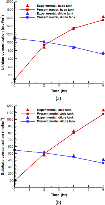
Figure 3. A comparison between the experimental data and present model results (a) lithium ion at LiOH and Li2SO4 tanks; (b) sulphate ions at the H2SO4 and Li2SO4 tanks.
Download figure:
Standard image High-resolution imageEffect of current density on the concentration distribution and transmembrane water velocity
Figures 4a and 4b respectively show the concentration distributions of lithium, and sulphate ions in the CEM, AEM and their vicinity diffusion boundary layers versus the dimensionless length. The inlet concentration of lithium ions at the dilute and concentrate base channels, which have been set 800 mol·m−3, and the sulphate inlet concentration of the dilute and concentrate acid channels, considered as 400 mol·m−3, are respectively shown as straight lines in Figs. 4a and 4b. As indicated in these figures, the ions concentration in the dilute compartment decreases toward the IEMs, while at the concentrate sides it rises toward the IEMs. In addition, in the membrane phase, the ions concentration at the concentrate channel side is greater than that at the dilute channel side. Furthermore, increasing the current leads to higher concentration gradients at IEMs and their adjacent solutions.

Figure 4. Concentration polarization profiles of regions around IEMs: (a) concentrate base-CEM-dilute channels; (b) dilute-AEM-concentrate acid channels.
Download figure:
Standard image High-resolution imageFigure 5 shows the magnitude of transmembrane velocity of water molecules passing through the AEM and CEM as a function of current magnitude. It is well known that in ED systems, water molecules penetrate through the membranes due to the electro-osmotic mechanism, which is related to concentration of counter-ions at IEMs as well as potential gradient across the membrane, as described by Eq. 5. Therefore, it is expected that increasing current leads to the enhancement of water velocity through IEMs, as presented in Fig. 5. The water velocity through CEM is greater than that of AEM due to higher voltage drop across CEM. Considering the average concentration of counter-ions at the membrane phase of solution-IEM interfaces as the concentration of counter-ions, which is directly dependent on transmembrane water velocity, the variation of transmembrane water velocity would follow a non-uniform trend.
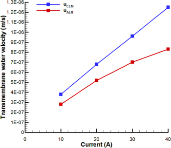
Figure 5. Variations of water velocity through CEM and AEM at different currents.
Download figure:
Standard image High-resolution imageEffect of inlet concentration of the dilute channel
Figure 6a compares the concentration variations of lithium and sulphate species stored respectively at the LiOH and H2SO4 tanks with respect to different initial concentrations of the Li2SO4 tank, cLi2SO4 0. Two initial concentrations of the Li2SO4 solution, i.e., 500 and 1000 mol·m−3 were considered, while the concentration of Li+ and SO4 2− were 100 mol·m−3 at the beginning of the experiments. As indicated in this figure, which shows a good agreement between experimental data and model results, increasing the cLi2SO4 0 results in a higher concentration of the LiOH and H2SO4 solutions, and this variation is more obvious for the LiOH solution.

Figure 6. Effect of the cSO4d in on the: (a) Li+ and SO4 2− concentration; (b) water velocity through the AEM.
Download figure:
Standard image High-resolution imageSince the present model is developed assuming constant current condition during the ED operation, the concentration of concentrate compartments is a function of water velocity through the IEMs. Increasing the initial concentration of Li2SO4 solution would leads to the reduction of the transmembrane water velocity and enhancement of the concentration of concentrate compartments. As evidenced in Fig. 6b, increasing the initial concentration of the Li2SO4 solution reduces the volume of the LiOH tank due to the reduction of water velocity through the CEM. Therefore, increasing the inlet concentration of species at the dilute channel improves the function of ED.
Effect of membrane properties on the water transport through the membrane
The effect of membrane characteristics, e.g., its thickness and water volume fraction, on the transmembrane water velocity across the CEM as well as outlet lithium concentration of the concentrate base channel are interest to practical application of ED. Figures 7a and 7b show the transmembrane water velocity and the outlet lithium concentration of the concentrate base channel as functions of membrane thickness and water volume fraction, respectively. As illustrated in these figures, the lithium concentration of the concentrate base channel increases by raising the thickness and water volume fraction of the CEM due to reducing the water velocity through the CEM. Moreover, these membrane parameters are more influential at lower values.

Figure 7. The variations of transmembrane water velocity and the lithium outlet concentration of the concentrate base channel in different (a) CEM thickness; (b) water volume fraction.
Download figure:
Standard image High-resolution imageEffect of counter-ion's size on the water transport through IEMs
The effect of counter-ion's size on the transmembrane water velocity and the outlet concentration of the concentrate base channel is shown in Fig. 8. One can see that larger particles results higher transmembrane water velocity and lower concentration in the concentrate channels. This phenomenon shows that larger species carry more water molecules through the IEMs in comparison with the smaller ones. Therefore, among lithium, sodium, potassium, rubidium, and caesium ions, the lithium ions have the lowest bare ion radius and can provide the highest membrane performance. It should be noted that these results are taken at the conditions presented in Table V.

Figure 8. Variation of the transmembrane water velocity through CEM and the outlet concentration of the base channel for different ions. The ions presented at vertical axis are arranged based on increasing their bare ion size and the properties of each ion, i.e., bare ion radius, R, 57 hydrated ion radius, HR, 58 and limiting ionic conductance in water at 298 K, Landa0, 48 are presented.
Download figure:
Standard image High-resolution image
Table V. Input parameters and modeling conditions during the parametric studies.
| Figure number | 4, 5 | 7, 8 | 6 | |
|---|---|---|---|---|
| Operation mode | Single-pass | Single-pass | Batch | |
| Concentration, mol·m−3 | LiOH | 800 | 800 | 100 |
| Li2SO4 | 400 | 400 | 500, 1000 | |
| H2SO4 | 400 | 400 | 100 | |
| Temperature, ℃ | 60 | 60 | 25 | |
| Current, A | 10, 20, 30, 40 | 20 | 28 | |
| Inlet flow rate, m3·s−1 | 0.555 × 10⁻⁶ | 0.555 × 10⁻⁶ | 5.55 × 10⁻⁶ | |
| CEM type | Fumasep FAA-3-PK-130 | Nafion NRE-212 | ||
| AEM type | Fumasep FKE-50 | Neosepta ACM | ||
Uncertainty propagation
In statistics, uncertainty propagation refers to the effect of input parameters uncertainty on the uncertainty of objective output parameters. In other words, to study how uncertainty in a calculated variable, which is known as an output of a numerical model, might be attributed to different input parameters. Considering amount of input parameters and their relative uncertainties, the uncertainty of the output objectives can be calculated as follows: 59

in which 
 and
and  are the uncertainty of output objectives, uncertainty of input parameters, and partial derivative of each parameter, respectively. The uncertainties of output objectives are obtained in percentage, and a higher uncertainty represents a greater influence of the corresponding input variable on the output parameter.
In the present study, uncertainty propagation is used to investigate the importance of studied input parameters, i.e., current, inlet concentration of the dilute solution, counter-ion radius, the thickness and porosity of CEM, on output objectives including water velocity through CEM and outlet concentration of the concentrate base compartment. Table VI presents the effect of input parameters on the base channel's outlet concentration and water velocity through CEM. As indicated in this table, the relative uncertainty of all input parameters is considered 50% to provide a better comparison among input parameters.
Table VI. The effect of input parameters on the uncertainty of output parameters.
| Input parameters | Output parameters | ||||||
|---|---|---|---|---|---|---|---|
| Value | Relative uncertainty, % | Absolute uncertainty | Li outlet concentration at base channel, mol·m−3 | Water velocity through CEM, m·s−1 | |||
| uncertainty, % | Effect | uncertainty, % | Effect | ||||
| Current, A | 34 | 50 | ±17 | 71.23 | ↑ | 40.30 | ↑ |
| Inlet concentration of dilute compartment, mol·m−3 | 1260 | 50 | ±630 | 5.00 | ↑ | 9.94 | ↓ |
| Counter-ion radius, pm | 60 | 50 | ±30 | 16.75 | ↓ | 34.69 | ↑ |
| Thickness of CEM, μm | 55 | 50 | ±27.5 | 1.24 | ↑ | 2.59 | ↓ |
| Water volume fraction of CEM, % | 40 | 50 | ±20 | 5.79 | ↑ | 12.48 | ↓ |
Based on Table VI, current is the most effective parameter among studied input parameters on both outlet concentration of the base channel and transmembrane water transport. However, the influence of current on the outlet concentration of base channel is significantly higher than its influence on the water velocity. Besides the current, the size of counter-ion, CEM water volume fraction and concentration of the dilute channel are the most important parameters affecting the objective parameters' uncertainty, respectively. Also, the effect of the counter-ion radius has higher impact on the transmembrane water velocity than concentration.
Conclusions
In this study, a comprehensive model for electrodialysis is developed and validated for both single-pass and batch configurations. The errors between the present model and experimental data for the single-pass ED was 5.5%, and for the batch configuration reported 3.5, 2.5, and 6.25% after 2, 4, and 6 h of ED running, respectively. Based on the validated baseline case, a parametric study was carried out to investigate the effects of various parameters on the performance of ED. When the applied current was increased, the concentration polarization increased at IEMs, and more water molecules were transferred within membranes. Also, increasing the Li2SO4 concentration entering the dilute channel from 500 to 1000 mol·m−3 led to a 15% increase of the concentration of the LiOH tank and a decrease of 13% solution volume of this tank after 5 h of ED operation, while no considerable variation was observed for the H2SO4 solution. In addition, the effect of membrane properties was studied on the membrane performance. The variation of thickness of CEM from 30 to 150 μm led to the reduction of 62% of transmembrane water velocity. Furthermore, increasing the water volume fraction of CEM increased the outlet LiOH concentration from 813 to 908 mol·m3. Around 80% of this increase occurred when the water volume fraction was enhanced from 10% to 30%. Moreover, by investigation of the various ions moving into CEM, it was concluded that ions with the larger bare ion radius carry more water molecules due to increasing transmembrane water velocity from 0.51 to 1.36 μm·s−1 by transferring lithium and caesium ions into the CEM, respectively. Finally, the importance of these studied parameters on the outlet concentration of base channel as well as transmembrane water velocity through CEM was investigated using the uncertainty propagation technique. It was found that current is the most influential parameter, which consists of about 70% base channel's outlet concentration uncertainty and 40% CEM water velocity uncertainty. In addition, the radius of counter-ions was the other important parameter considerably affecting water velocity uncertainty.
Acknowledgments
This work was supported by the National Natural Science Foundation of China (No. 21776226) and the China Scholarship Council (2019SLJ017820). The authors acknowledge the support of experimental facilities from the Energy Internet Research Institute of Tsinghua University, Chengdu, China.