
Abstract
Cylindrical lithium-ion batteries are used across a wide range of applications from spacesuits to automotive vehicles. Specifically, many manufacturers are producing cells in the 18650 geometry i.e., a steel cylinder of diameter and length ca. 18 and 65 mm, respectively. One example is the LG Chem INR18650 MJ1 (nominal values: 3.5 Ah, 3.6 V, 12.6 Wh). This article describes the electrochemical performance and microstructural assembly of such cells, where all the under-pinning data is made openly available for the benefit of the wider community. The charge-discharge capacity is reported for 400 operational cycles via the manufacturer's guidelines along with full-cell, individual electrode coating and particle 3D imaging. Within the electrochemical data, the distinction between protocol transition, beginning-of-life (BoL) capacity loss, and prolonged degradation is outlined and, subsequently, each aspect of the microstructural characterization is broken down into key metrics that may aid in understanding such degradation (e.g., electrode assembly layers, coating thickness, areal loading, particle size and shape). All key information is summarized in a quick-access advanced datasheet in order to provide an initial baseline of information to guide research paths, inform experiments and aid computational modellers.
Export citation and abstract BibTeX RIS

This is an open access article distributed under the terms of the Creative Commons Attribution 4.0 License (CC BY, http://creativecommons.org/licenses/by/4.0/), which permits unrestricted reuse of the work in any medium, provided the original work is properly cited.
Commercial lithium-ion (Li-ion) batteries are produced in several geometries but can generally be assigned to one of the following: coin, pouch, prismatic or cylindrical.1,2 With the latter three currently holding the majority of the market space. Specifically, cylindrical cells have proven popular with certain automotive manufacturers for battery electric vehicles (BEVs) due to many factors including: cost, ease of cooling, the mechanical strength of the steel casing, and the ability to demonstrate a degree of control in gas ventilation during failure.3 The 18650 has become a commercial standard for cylindrical cells i.e., a cylinder of diameter and length ca. 18 and 65 mm, respectively, and cell manufacturers are producing various chemistries and vent geometries in this format.1
The pairing of high capacity (e.g., around 0.2 Ah g−1 and 1 Ah cm−3) electrodes that operate with a large potential window, (e.g., 3.0–4.2 V) produce favourably high on-board energy storage (ca. 10–15 Wh per cell).1,2 For example, assembling layered transition metal oxide cathodes, such as LiNixMnyCozO2 (NMC), with graphite-silicon composite anodes presents one of the most promising chemistries for the automotive sector. However, each electrode still suffers performance loss due to several complex degradation mechanisms: NMC is susceptible to parasitic reactions with the electrolyte, cation mixing, surface restructuring, active material dissolution, oxygen release and inter-granular cracking4; whereas silicon anodes suffer from significant volume expansion,5 requiring novel micro- and nano-structures to minimise undesirable mechanical stress,6 and when fabricated as composites with graphite, can lead to significant charge balancing during open circuit.7 It is therefore important to study the performance (and failure) of such promising chemistries in order to understand, and mitigate, their degradation during operation.
Due to the intimate relationship between microstructure and electrochemical performance, X-ray computed tomography (CT) methods have revolutionized the field of Li-ion materials characterization.8 Moreover, a growing number of communities are working together in order to pursue unified goals, e.g., "the million-mile battery"9; consequently, greater efforts are being made to improve data transparency and sharing,10 particularly to investigate promising materials such as nickel-rich NMC811 cathodes and high capacity silicon-graphite anodes. One commercial cell type that employs such chemistries is the INR18650 MJ1 (LG Chem Ltd. Korea), and several studies exist within the literature on this cell-type.11–15
Multi-length-scale analysis has proven highly valuable for other chemistries16; however, to the authors' knowledge, there is no report of multi-length scale microstructural data coupled with electrochemical cycling information on the MJ1 cell type (INR18650: NMC811 vs graphite-silicon). Consequently, the primary motivation of this work is to release a comprehensive study and the accompanying raw data obtained from commercial MJ1 cells in order to aid the wider community by providing a baseline for computational modelling, inform future degradation investigations and generally open discussions for research motivations and directions. The format of this paper is intended as a "template" for the open source sharing of cell data via advanced datasheets.
Experimental
Materials
All data in this work were obtained from LG Chem INR18650 MJ1 cells (Nkon, Netherlands) and the manufacturer's specifications can be found within Table SI (available online at stacks.iop.org/JES/167/140530/mmedia). Although the electrode materials are not stated on the manufacturer's specifications, the printed anode and cathode electrodes have been previously confirmed to consist of a silicon-carbon composite and NMC811 (LiNi0.8Mn0.1Co0.1O2).12
Electrochemistry
Electrochemical cycling was achieved using a Maccor 4200 cycler (Maccor Inc. U.S.A.). Charging was performed using a constant-current-constant-voltage (CC-CV) charge protocol, where the cell was held at a constant current of 1.5 A until 4.2 V, then a constant voltage of 4.2 V was held until the current decreased to 100 mA. Discharging was performed with a single CC step at 4.0 A to a discharge cut-off voltage of 2.5 V. Nominal specifications can be found in Table SI with protocol details in Table SII. This protocol was followed for 400 cycles as recommended by the manufacturer's high drain protocol however there were relaxation interruptions in the cycling when the cell reached certain capacity values (e.g., 90%, 88%, 86%, etc.,). Where data is plotted with respect to cycle number, interruptions are indicated by vertical dashed lines and labels. All cycling was performed within an environmental chamber set to 25 °C, although cell temperatures were recorded to increase above this, particularly during points of high current due to Joule heating, consequently the average cell temperature for each cycle was closer to 30 °C, however high-temporal resolution surface temperature data is available via the data repository, i.e., data with time frequency of per second rather than per cycle. All raw cycling data (capacity, cell potential, cell temperature, coulombic efficiency) can be found within the accompanying DiB article17 and is free to download from the data repository.18
The coulombic efficiency was calculated as the discharge capacity for the nth cycle (cycle number n) divided by the charge capacity for the same cycle number. The differential capacity (dQ dV−1 presented in units of Ah V−1) was calculated from the smallest increments in the cell potential and capacity, as supplied in the raw data. The differential capacity peak-height noted "I" in the subsequent text, was calculated as the point where the average gradient of the differential capacity plot was closest or equal to zero, and the gradient before and after averaged a positive and negative value, respectively. Throughout, the capacity loss was defined as the difference between the capacity, e.g., charge capacity, for cycle n and n + 1. Finally, the integration of the differential capacity curves was achieved using MATLAB software (Mathworks, Cambridge, U.K.) by defining 5 voltage regions of interest (RoI) that correspond to: 1. the onset of bulk charge transfer (<3455 mV); 2. the aforementioned Peak I (3455–3650 mV); 3. Peak II (3650–3900 mV); 4. Peak III (3650–4140 mV); and 5. the upper voltage threshold (>4140 mV). In order to obtain a capacity value for each voltage RoI, the differential capacity charging curve was integrated with the stated voltages as limits. As the differential capacity tends to infinity during the CV step (i.e., dV ∼ 0), the capacity for the final voltage RoI (V > 4140 mV) was obtained by subtracting the capacities for the other 4 voltage RoIs from the total cell charging capacity.
X-ray CT
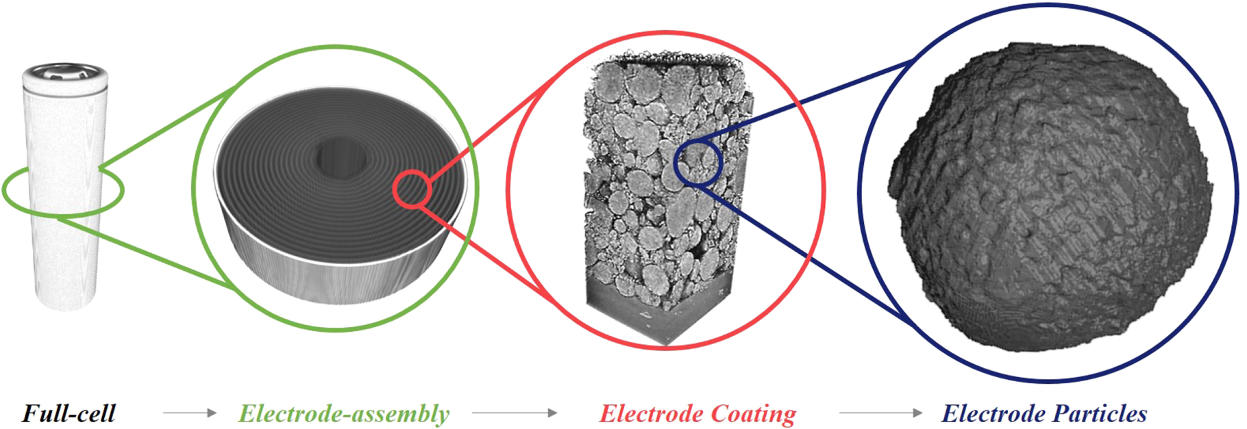
The structural data presented here can be subdivided by length-scale: the full-cell, electrode assembly, printed electrodes and electrode particles. This is visualised by examples in Fig. 1. All of the 3D datasets were obtained from commercial laboratory X-ray computed tomography (CT) instruments, the imaging procedure for each length-scale will now each be sequentially described. Firstly, one 3D image was collected of the full-cell with a spatial RoI encompassing the entire cell i.e., 20 × 20 × 72 mm3. This was achieved using a Nikon XT H225 instrument (Nikon Metrology, Inc. U.S.A.) with a 58 keV (W-Kα) cone-beam producing a tomogram with an isotropic voxel length of 36.0 μm. Secondly, four 3D images of the electrode assembly with a spatial RoI encompassing 5 mm of cell length and the entire cell diameter i.e., 20 × 20 × 5 mm3. These were collected using a 520 Versa instrument (Zeiss Xradia 520 Versa, Carl Zeiss., CA, USA) with a 58 keV (W-Kα) cone-beam producing a tomogram with an isotropic voxel length of 10.4 μm. Thirdly, two 3D images of the printed electrodes and electrode particles with a spatial RoI encompassing the full electrode thickness e.g., 115 μm and a small area ca. 64 × 64 μm2. These were collected using an 810 Ultra instrument (Zeiss Xradia 810 Ultra, Carl Zeiss., CA, USA) with a 5.4 keV (Cr-Kα) quasi-parallel beam producing a tomogram with an isotropic voxel length of 63.1 nm. This instrument employs a capillary condenser to focus the X-rays for a full-field illumination of the sample where the transmitted beam is projected onto a scintillator detector using a Fresnel zone plate.

Figure 1. Defining the length-scales of interest for multi-length-scale microstructural characterisation: full-cell, electrode assembly, electrode coating and particles.
Download figure:
Standard image High-resolution imageTo optimise the data quality obtained from the printed electrodes, the cathode was imaged using Zernike phase-contrast, where a phase-ring was inserted into the beam-path to emphasize edge features, whereas the anode was imaged without the use of the phase ring, i.e., absorption dominated, in order to maximize the contrast between the silicon and the carbon. This is contrary to typical practice; generally, light materials (e.g., anodes) are imaged with phase-enhancement whereas more attenuating materials (e.g., cathodes) are imaged with absorption-dominated methods. However, the use of a phase-ring generally does not provide purely phase information, i.e., images are produced through a mixture of absorption and phase X-ray interactions with the sample, and provides enhanced edge detail for features such as cracks (as are often seen within Li-ion cathodes) while also allowing sufficient contrast to distinguish the cathode particles from the other matter within the RoI, e.g., carbon, binder and void. Moreover, the large attenuation difference between the silicon and carbon materials within the anode were best suited to absorption imaging in order to maximise image contrast for segmentation; although both phase and absorption information may be gained when imaging with a phase-ring, the segmentation of the two active materials (silicon and graphite) was of particular interest thus required maximum image contrast i.e., absorption.
All data was reconstructed using commercial software employing filtered-back-projection (FBP) algorithms (full-cell CT: "CT Pro 3D," Nikon Metrology, Inc. U.S.A.; electrode assembly, anode and cathode CT: "Reconstructor Scout-and-Scan," Carl Zeiss., CA, U.S.A.). In order to capture the full electrode thicknesses, each CT of the printed electrode coating required the collection of two tomograms vertically (in the z-plane) that were then computationally stitched after reconstruction. A full list of the imaging parameters can be found in Table I, and within the accompanying Data in Brief article.17 Moreover, all 3D data is free to download from the data repository.18
Table I. Multi-length-scale X-ray CT acquisition and reconstruction parameters.
| Electrodes Coating & Particles | ||||
|---|---|---|---|---|
| Full-cell | Electrode Assembly | Anode | Cathode | |
| Instrument | Nikon | Zeiss Xradia | Zeiss Xradia | |
| XT H225 | 520 Versa | 810 Ultra | ||
| Tube Voltage | 170 V | 120 V | 30 V | |
| Beam Energy | 58 keV | 58 keV | 5.4 keV | |
| Monochromaticity | Polychromatic | Quasi-monochromatic | ||
| Beam Geometry | Cone | Parallel | ||
| Projections | 2,278 | 4,500 | 2,400 | 1,200 |
| Exposure time | 1 s | 10 s | 30 s | 60 s |
| Data stitching required | No | Yes: 2 tomograms vertically | ||
| RoI | 21 × 23 × 73 mm | 21 × 21 × 5 mm | 64 × 65 × 95 μm | 64 × 71 × 112 μm |
| Voxel Length | 36.0 μm | 10.4 μm | 63.1 nm | |
| Absorption/Phase | Absorption | Phase | ||
| Repository dataset | EIL-016 | EIL-005 | EIL-013 | EIL-014 |
| EIL-006 | ||||
| EIL-007 | ||||
| EIL-008 | ||||
SEM and EDX
Complementary scanning electron microscope (SEM) imaging and energy dispersive X-ray mapping (EDX) was conducted using an EVO MA 10 SEM (Carl Zeiss, USA) and is provided within the supplementary section (Figs. S2 and S3) with the specific imaging parameters noted on each image.
Data analysis
Visualization and quantifications were achieved using Avizo Fire (Avizo, Thermo Fisher Scientific, Waltham, Massachusetts, U.S.A.), Fiji (ImageJ, U.S.A.), Python (Python Software Foundation, PSF) and MATLAB (Mathworks, Cambridge, U.K.) software.
The electrode thicknesses were assessed from the full-cell CT using a virtual unrolling algorithm previously developed by Kok et al. that employs a Python script to virtually unroll the structure for analysis, details of which are described thoroughly elsewhere.13 This method quantified a thickness for: "A" the double-layered cathode with Al current collector, and "B" the separators and the double-layered anode with Cu current collector. The separator and anode are assessed together at this length-scale due to their similarly low attenuation coefficients. To repeat these quantifications see dataset: EIL-016.tif in the data repository.18
To conduct a high-resolution analysis of the electrode assembly, the cell was visualized with a greyscale ortho-slice and accompanying greyscale histogram using Avizo. A greyscale line-scan used to demonstrate the electrode assembly layers was collected using ImageJ with a 5-pixel line-width average. The line-scan was taken from outside of the cell (i.e., void/air) to the cell centre (i.e., electrolyte). Eleven line-scans were taken at ca. 10 μm vertical increments and overlaid in order to assess vertical greyscale variation within the tomogram. To repeat these quantifications see dataset: EIL-005.tif, EIL-006.tif, EIL-007.tif or EIL-008.tif in the data repository.18
The printed electrode tomograms were visualized using greyscale ortho-slices and greyscale volume renders using Avizo. In order to quantify metrics from the electrodes, the greyscale data was segmented. Regardless of the segmentation algorithm used, the current collector was first cropped manually from the data, to do this, the data was aligned so that the current collector/electrode interface was perpendicular to the voxel structure, i.e., the interface was at approximately the same vertical position in z for all values of x and y. To repeat any electrode- or particle-level quantifications see datasets: EIL-013.tif and/or EIL-014.tif in the data repository.18
The cathode could be segmented into a binary dataset of NMC and other material (i.e., where the "other material" is considered as one phase containing: void, carbon and binder) using a simple grayscale threshold due to the large difference between the attenuation coefficient of the NMC and the lighter components: carbon, binder and void. The anode segmentation was more complex; the combination of multiple independent tomograms can often lead to subtle variations between greyscale values of the same material within the stitched tomogram, particularly for very lowly attenuating elements e.g., graphite, carbon or void. Therefore, applying a threshold to the greyscale histogram often results in an inaccurate segmentation and thus has been avoided here. To mitigate these errors, localized greyscale operations were employed. Firstly, to segment the silicon material, a localized bright top-hat transform was conducted, which due to the large image contrast between the relatively dark greyscale of the graphite/void with the bright greyscale of the silicon, successfully detected all of the silicon particles, producing tomogram 1. Secondly, to segment the pore from the graphite material, a localized dark top-hat transform was conducted producing tomogram 2. This successfully detected small (i.e., submicron) inter- and intra-particle voids but did not sufficiently detect large external voids (i.e., with diameters of several microns). The greyscale anode tomogram was then filtered substantially in Avizo, by resampling the data (a "resample" filter which averages local voxel values into one, larger voxel) equivalent to a binning of the voxel length from 63 nm to 630 nm. This removed variation in the greyscale values throughout the graphite at the cost of resolution, but still with sufficient detail for characterizing the large external voids. The binned dataset was then segmented using a greyscale threshold producing a very low resolution binary graphite tomogram 3. This tomogram was then applied as a mask to the void tomogram 2, whereby all values within the binned tomogram 3 that didn't corresponded to graphite (e.g., void, silicon, etc.) were subtracted from void tomogram 2, producing tomogram 4. This produced an accurate map of the whole pore structure plus the silicon material, however, as the silicon had already been segmented in tomogram 1, subtracting the silicon material within tomogram 1 from tomogram 4 produced tomogram 5: a three-phase tertiary tomogram containing silicon, graphite and void. All segmentation was conducted using Avizo software.
The material compositions (vol%) were calculated using the summation of all voxels containing a material of interest after segmentation, divided by the total number of voxels within the spatial RoI. It should be noted that the spatial RoI originally obtained during the X-ray imaging (stated in Table I) had generally reduced by the point of completing the segmentation and data processing. These computations were achieved using both MATLAB and Avizo Fire, producing identical solutions.
After segmentation, the electrode thickness could be quantified by summing all voxels containing electrode material in the z-plane for a particular x-y position. This produces one z-projected 2D image that represents the local electrode thickness. Taking the mean of this map produced the average electrode thickness. In order to calculate the local loading, the crystallographic density for each material was used as an approximation for the local volumetric mass density,19,20 producing a mass per unit area. And finally, the theoretical capacity for a particular operational voltage, e.g., 4.2 V, was used to calculate the local and average areal capacity. All thickness, loading and areal capacity calculations were computed using MATLAB. To visualize the 3D structures, triangulated surfaces were computed from the cubic voxel-based binary or tertiary data for each material. All surfaces were generated using Avizo. The anode feature sizes were quantified with line-scans using ImageJ and centroid-path skeletons using Avizo.
Particle quantifications were obtained by assigning each individual particle within the segmented tomograms with a unique number label using a connected-objects separation and label analysis. This produced a volume and area for each particle. An equivalent diameter was then calculated from the volume of each particle for a sphere of equal volume. The sphericity was quantified from the ratio of the particle surface area and the surface area of a sphere with an equivalent volume. Histograms were then calculated using MATLAB.
Results
Electrochemical information
The first five electrochemical charge-discharge cycles for an LG Chem INR 18650 MJ1 cell are displayed within Figs. 2a and 2b, respectively, to examine the beginning-of-life (BoL) performance. These plots are highly consistent and show minimal variation between cycles. In order to observe the subtle differences with cycling, the differential capacity has been plotted within Figs. 2c and 2d with respect to cell potential. It can be seen that there is an initial peak "I" within the differential charge capacity curve that is substantially higher during the first cycle, compared to the subsequent four cycles. This is highlighted further in Fig. 2e where the differential capacity peak-height is plotted with respect to cycle number. To examine the cell's capacity retention, the charge and discharge capacities are plotted in Fig. 2g, with the coulombic efficiency displayed within Fig. 2h. The large increase in efficiency from cycle 1 to 2 is highlighted by the capacity loss with respect to cycle number, displayed within Fig. 2i. Comparing Figs. 2e and 2i, it can be seen that poor coulombic efficiency during low cycle numbers may be largely attributed to peak "I". For low cycle numbers this peak may often be associated with solid-electrolyte-interphase (SEI) formation within the anode,21 however, commercial cells are "formed" before dispatch therefore the likely cause of capacity loss here is the lack of Li+ inventory due to the change in the charge/discharge protocol between the formation and operation cycles. For instance, formation cycles are generally conducted at very low currents, e.g., 0.2 C, whereas operational cycles are conducted at higher currents, e.g., 1 C, in order to emulate real-world scenarios. During the last formation-discharge of the cell prior to the operational cycles reported in Fig. 2 (i.e., the formation cycle occurring before operational cycle 1), the cathode would have been lithiated slowly due to the low-current discharge, resulting in a large Li+ inventory within the cathode, and a highly delithiated anode. This inventory was accessed during the first operational charge (i.e., charge cycle 1 in Fig. 2) resulting in a large charge transfer to the anode and consequently a high peak-height, specifically peak I. However, due to the subsequent high-current discharge (i.e., discharge cycle 1 in Fig. 2) the cathode was not lithiated (and the anode was not delithiated) to the same state as it was during the formation (i.e., during the formation-discharge cycle). Therefore, during the next charge (i.e., charge cycle 2 in Fig. 2) there is less charge-transfer into the anode, thus consequently a lower differential capacity peak height. Through this reasoning, the initial capacity loss can be attributed to the protocol change between formation and operational cycling. Similarly the Columbic efficiency for the first operational cycle is not greatly informative due to the transition between formation and operation protocols, especially when comparing to higher cycle numbers (e.g., 2, 3, 4, etc., ...), however it is important to note this loss in Li+ inventory when transitioning to higher C-rate regimes. Reports of lower (<99%) Columbic efficiencies during early-stage cycling are not uncommon for NMC chemistries and particularly, NMC811-Graphite is known to evolve gas during operation22; specifically: carbon-, hydrogen- and oxygen-based compounds, e.g., C2H4, CO2, H2, CO and O2. Therefore as well as protocol transitions, lower early-stage Columbic efficiencies may also be a product of such gas evolution and can be studied by on-line electrochemical mass spectrometry (OEMS) however, as the aim of this work was to maintain operation as close as possible to real-world application (i.e., without cell disassembly) OEMS methods therefore exceed the scope of this article but a comprehensive study of gas evolution can be found by Jung et al.22
To further examine capacity variation with cycling, Fig. 3 plots cycling data extended to 400 operational cycles. It should be noted that, in addition to the top- and bottom-of-charge rest periods during cycling, the cycling was paused for several points of capacity retention (i.e., 90%, 88%, 86%, 84% and 82% of the initial capacity). This is highlighted by the plot of the cell surface temperature in with cycle number Fig. 3a, whereby each cycling period is coloured separately. Figures 3b and 3c supply extensions of Figs. 2g and 2h. To build upon this, Fig. 3d displays the charge and discharge capacities with respect to the first operational cycle. Within this plot the charge profile is seen to drop and remain lower due to the aforementioned losses associated with the transition from formation- to operational-cycling protocols. It can however be seen that although there is a substantial initial loss (possibly associated with the protocol change and potential gas formaiton), the capacity continues to decline with cycle number, during the BoL capacity declines quickly (the first ∼50 operational cycles) but continues to gradually decline up to the end of cycling (400 cycles). Figure 3e aims to clarify the difference between the various stages of capacity loss: firstly initially losses due to the protocol change (cycle number 1), secondly the early BoL losses (no clear ending although losses become less substantial after ∼50 cycles), and thirdly the long-duration degradation after prolonged cycling (up to 400 cycles). Moreover, the cell capacity losses can be roughly approximated by the power law that is overlaid on the figure. For computational purposes this approximation may be useful for the modelling community.
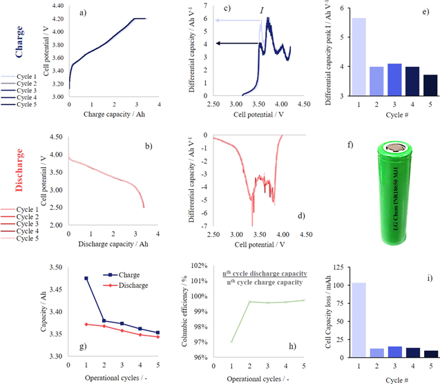
Figure 2. Early-stage electrochemical cycling of an INR 18650 MJ1 Li-ion cell: (a) charge and (b) discharge potential/capacity profiles, with accompanying (c) charge and (d) discharge differential capacity profiles; (e) differential charge capacity peak-height for peak I with cycle number; (f) a photograph of the cell; (g) charge and discharge capacity, (h) columbic efficiency and (i) cell capacity loss all plotted with respect to cycle number.
Download figure:
Standard image High-resolution image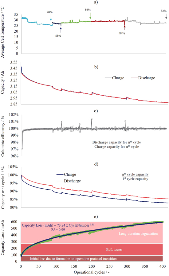
Figure 3. Long-duration electrochemical cycling of an INR 18650 MJ1 Li-ion cell: (a) cell surface temperature, (b) capacity, (c) coulombic efficiency, (d) capacity retention, and (e) capacity loss, all plotted with respect to cycle number. The arrows noted on (a) indicate pauses in electrochemical cycling.
Download figure:
Standard image High-resolution imageFigure 4a displays the differential charge capacity (as was seen in Fig. 2c) for the first and every subsequent hundred cycles. Highlighted within the figure are four of the five voltage RoIs: the onset of charge transfer (green), peak I (light blue), peak II (dark blue) and peak III (red). The initial onset of charge transfer at low voltages can be seen to creep to higher cell potentials with cycle number, this is displayed through the magnified sub-plot of the minimum cell potential where current was greater than 0 A versus the operational cycle number (Fig. 4b). Arrows have also been added to highlight changes that occur quickly at the BoL (white/blue arrows) and slowly over the long-duration cycling (red/black arrows). The four regions are magnified for closer inspection in Fig. 4c. As described in Fig. 4b, the onset of charge transfer creeped to higher cell potentials with increasing cycle number. Moreover, peak I was considered in Fig. 2e and, as observed previously, the peak-height decreases considerably after the first cycle (BoL), and remains at the lower value for subsequent cycles. Peaks II and III are thought to be associated with the NMC cathode12,23,24 and there are also BoL losses from the early cycling observed within these peaks; however, they are far less substantial. Moreover, both peak heights are also observed to decrease gradually with the long-duration cycling, suggesting prolonged degradation of charge transfer mechanisms associated with the cathode that reduce the degree of Li+ mobility, possibly in the form of particle cracking or surface reactions.4

Figure 4. Differential charge capacity analysis of an INR 18650 MJ1 Li-ion cell up to 400 operational cycles: (a) full differential charge capacity profile for cycles 1, 100, 200, 300 and 400; (b) the minimum cell potential at which the cell current rose above 0 A with respect to operational cycle number (dashed vertical lines indicate pauses in cycling); (c) four of the voltage RoIs highlighted and magnified for analysis.
Download figure:
Standard image High-resolution imageTo explore the charge curve with a higher temporal resolution, the differential capacity curve was integrated for each of these four regions: the low voltage onset of charge transfer, peaks I, II and III, and upper voltage cut-off. This produced a charge capacity for each voltage RoI with respect to cycle number, these are displayed individually within Fig. 5a and combined within Fig. 5b as a percentage of the total charge capacity. This highlights the repercussions of the variations observed within the differential capacity profiles within Fig. 4a. The delayed onset of charge transfer at low voltages results in a reduced charging capacity below 3.5 V. The substantial reduction in the height of peak I at low cycle numbers causes a decline in charge transfer between 3.5–3.7 V that levels into a near-linear decline after tens of cycles. Although there is an initial reduction in the charge transfer associated with peaks II and III, it is not as substantial as peak I and the reduction of peak III with cycling is negligible compared to the other three regions. For completeness, the capacity contribution for the upper voltage cut-off is also supplied (Figs. 5a and 5b in grey). Figure 5c compares the capacity losses associated with the delithiation of the cathode (summation of the capacity associate with peaks II and III) and the lithiation of the anode (I) during charging. From the figure it appears that the capacity losses associated with the anode and cathode both increase however, also diverge with cycle number. It can also be see that the pauses in electrochemical cycling may cause considerable jumps in performance (dashed vertical lines in Figs. 5b and 5c).

Figure 5. Assessing long-duration electrochemical cycling implications on the capacity of INR 18650 MJ1 Li-ion cells: (a) the five voltage RoIs assessed individually with the same y-axes scale to give an indication of degradation significance; (b) the breakdown of capacity contributions for the 5 voltage RoIs with respect to the total charge capacity; and (c) the approximated contribution of the charging capacity losses associated with the delithiation of the cathode and lithiation of the anode. Dashed vertical lines indicate pauses in the electrochemical cycling.
Download figure:
Standard image High-resolution imageElectrode degradation is complex and currently forms the basis of several large multinational investigation efforts. The authors have supplied all raw electrochemical data via the data repository18 as described within the accompanying Data in Brief article.17 We encourage readers to download the data and, where possible, perform further analysis of these metrics in order to further probe the complex degradation mechanisms at play. For instance, this differential capacity analysis may be extended through the use of machine learning algorithms,25 comparisons to electrochemical simulations,12,26 or in evaluation to future experiments on similar chemistries.
Cell-level information
The electrochemical performance of a cell is known to be strongly influenced by the cell microstructure and has associated performance losses that span multiple length-scales.16 Progressing from the electrochemical data and onto the full cell structure, Fig. 6a displays an ortho-slice from the tomogram of the entire cell assembly.19 The individual cell components (double-layer electrodes, steel casing, etc.) can be seen within the slice, distinguished by greyscale variations along the cell radius (Fig. 6b). Variations in greyscale values within a tomogram can be problematic, particularly for cone-beam geometries that are imaging at the limits of the system/instrument, as was the case in this work. Cone-beam geometries at the limit of their resolution capabilities can result in insufficient information at the detector edges, producing sections of incomplete information within the sinogram. Consequently, it is common to observe artefacts at the z-limits of the tomogram, i.e., with the top and bottom slices of the 3D volume, and therefore, the volumes must be cropped sufficiently to be free of artefacts. To ensure that this was the case, a line-scan was taken from point i to ii to quantify potential undesired variations, and was collected at various heights to examine greyscale consistency (see z-plane in Fig. 6a for geometric reference). The magnified plot of the peak associated with the steel casing further demonstrates this, where under 2% greyscale variation can be observed in the z-plane. It can be concluded that negligible variation is observed in greyscale with respect to height, i.e., the greyscale associated with a particular material, e.g., the steel casing, is consistent throughout the tomogram and global greyscale analysis can be conducted.

Figure 6. Full-cell and electrode assembly data collected from an INr 18650 MJ1 Li-ion cell: (a) a reconstructed 3D volume from the full-cell data and accompanying cross-sectional ortho-slices taken from the electrode assembly data, with (b) accompanying greyscale line-scan from points i to ii, (c) average greyscale values associated with each of the cell components, and (d) the approximate component thicknesses for the two layers A and B, as described in the accompanying diagram.
Download figure:
Standard image High-resolution imageFigure 6c displays the average greyscale values presented for each cell component: void, electrolyte, Cu current collector, silicon-graphite anode, NMC cathode, Al current collector and steel casing. It should be noted that the difference between the separator and the anode material is not accurately distinguishable at this resolution and is therefore not reported, this is a signal- and contrast-to-noise issue, as discussed in other work.20 Due to consistency in the greyscale data (as outlined in Figs. 6b and 6c) the electrode thicknesses could be approximated using a virtual unrolling technique.13 For this method, the assembly was consolidated into two sections: "A" and "B". A consisted of the double-layer cathode and current collector, and B the double-layer anode, current collector and two separators. Figure 6d displays the thickness distribution for these two sections; the thickness of A and B are approx. 150 μm and 210 μm, respectively. To collect this data, several thousand (∼2000) thickness measurements were collected per section, giving confident statistics in the outcome. However, as with most spatial quantifications, the precision of the raw data has an impact on the accuracy of the quantifications; the spatial resolution of the tomogram dictates the accuracy of these thickness measurements. The tomogram isotropic voxel lengths of the full-cell and electrode assembly data are 36.0 μm and 10.4 μm, respectively; the latter is one of the highest reported for an entire electrode assembly using lab-based image,27 however, to investigate the electrode morphology further the authors extend this investigation using nano-CT with substantial improvements to spatial resolution (with an isotropic voxel length of 63.1 nm).
Electrode-level information
The electrode-level characterization now continued into the printed anode and the cathode coating layers. Both electrodes were imaged at the same resolution to maximize compatibility for any future computational modelling that may be applied to the data from the repository.4,24 Figure 7 displays the greyscale ortho-slices with accompanying 3D volumes taken from each electrode, annotated to indicate features of interest (FoI).
Firstly, the anode contains two chemical components that are distinct due to their highly contrasting attenuation coefficients. It has previously been reported that these MJ1 anode materials can contain silicon compounds (e.g., SiOxwhere x may equal 0, 1 or 2, etc.).12 For a 5.4 keV incident beam, the attenuation length of pure Si, SiO2 and C6 are approx. 22, 40 and 500 μm, respectively.20 Consequently, within the tomogram, Si-based materials should appear considerably brighter (more attenuating) and can, therefore, be readily segmented from the lowly attenuating graphite (which is carbon-based) and voids. Moreover, the attenuation length of air (voids) is on the order of 20 cm, considerably higher than carbon, allowing the porosity to be segmented. There are slight variations in the greyscale values between the top and bottom halves of the anode tomogram due to minor inaccuracies in the post-acquisition data stitching and the increased noise levels due to the current collector in the lower volume. This is highlighted in Fig. 7 and is sufficiently minor to not prevent accurate segmentation via the algorithms discussed within the experimental section. Although EDX mapping detected oxygen in the same regions as silicon, the authors deemed EDX and greyscale analysis inconclusive as to the degree of oxygen within the Si-based material, i.e., whether it was pure Si, or an silicon oxide where x > 0, or some combination (Figs. S3 and S4 within the Supplementary Material). It is likely that the material contains a distribution of oxygen content both between particles and within individual particles and would therefore encourage readers to examine the existing data and conduct new experiments potentially through the use of advanced characterization methods such as X-ray absorption near-edge spectroscopy (XANES) and X-ray diffraction,28,29 and perhaps not only at the BoL, but also during, and after operation.
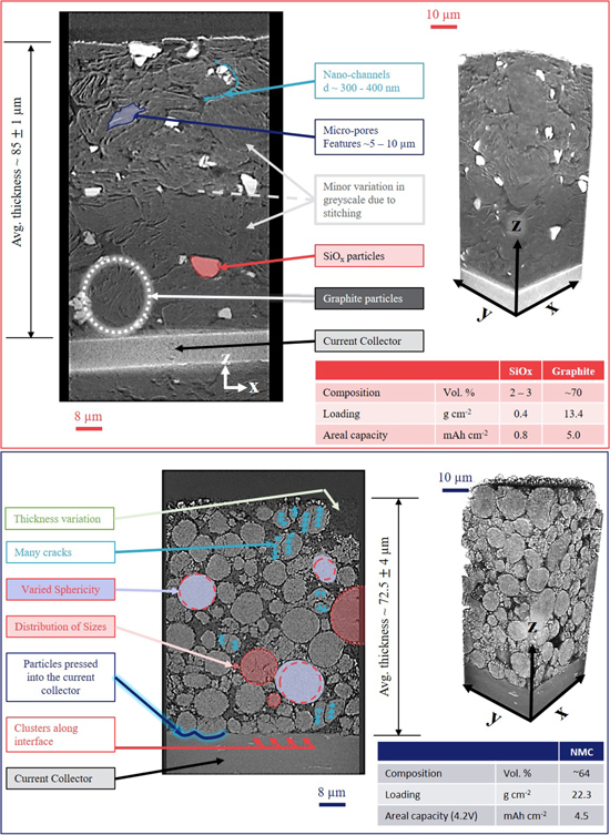
Figure 7. Electrode-level data collected from an MJ1 18650 cell: top) anode and bottom) cathode.
Download figure:
Standard image High-resolution imageThere are several microstructural features within the anode that may be of particular interest. The void-channels between the large graphite particles are on the order of 300–400 nm, these converge at micro-sized voids on the order of 5–10 μm. Figures S5 and S6 display the quantification of the graphite features through line scans and centroid-path skeletons, respectively. The silicon particles are of a similar scale to the voids, whereas the graphite particles are much larger, generally 10–20 μm. Particle sizes are assessed more thoroughly in the subsequent section.
The segmented graphite-silicon-void data was used to calculate the composition, electrode thickness, loading and areal capacity (for operation to 4.2 V). The average electrode thickness was measured to be ca. 85 μm with minimal variation ( 1 μm) (additional information within the Supplementary Material, Fig. S7). The silicon content has previously been reported to be around ∼5 wt%.12 The segmentation here resulted in a 2.2 vol% silicon content, equating to approx. 3–4 wt%. This offset may be attributed to local variation in cell composition. The silicon material was found to cluster along the edges of graphite particles, i.e., the mass loading of the silicon within the anode varied considerably (Fig. S8). Although the average mass loading of silicon was found to be 0.4 g cm−2, some areas exhibited over 2.5 g cm−2 (visualized within Fig. S8). This variation was not only observed parallel to the electrode-current collector interface (the x-y plane) but also with electrode thickness (the z-plane). As mentioned, the silicon content averaged 2.2 vol%; however, this value undulated considerably (between 1–6 vol%) throughout the electrode thickness, peaking near the separator-electrode interface (Fig. S9). Thus, surface measurements may over-predict the silicon loading, without the use of 3D analysis such as X-ray CT to expose sub-surface detail. Due to the particle size and distribution, the graphite loading was found to be significantly more consistent: ca. 13.4 g cm−2. Moreover, as both loadings have been determined, it can be concluded that approx. 1/6 of the capacity of the anode is supplied by the silicon, and the average anode areal capacity is ca. 5.8 mAh cm−2.
Through analysis of the greyscale values, the cathode was found to only contain one active material, which has previously been reported to be NMC811.12 Many of these NMC particles (>10%) exhibit crack features. Given that this structure was obtained prior to electrochemical cycling with minimal mechanical stress during X-ray sample preparation,30,31 these cracks may be attributed to calendaring.32 Moreover, several particles can be seen to have clustered along the electrode-current collector interface, with some even pressed into the current collector. There are various sizes of NMC particles (2–20 μm) and they generally display a high degree of sphericity (∼0.8); metrics such as this will be inspected more thoroughly within the subsequent section.
Unlike the anode thickness, which was seen to be highly consistent (∼85 μm), the cathode is thinner ca. 72.5 μm on average, and displayed regions of considerable variation of >5 μm where it appeared particles had been lost from the electrode surface (Figs. S10–S12). The authors postulate that this may occur due to preferential adhesion of particles to the calendaring device rather than particles to other particles via binder material in the coating; however, this would require further study for a confident conclusion and may form the basis of a time-resolved calendaring experiments to be conducted in the future. The segmentation of the active material from the cathode microstructure concluded an average loading of 22.3 g cm−2 and areal capacity of 4.5 mAh cm−2 for operation to cell voltages of 4.2 V. It should, however, be considered that calculating the local areal capacity of an electrode with respect to a particular cell potential may not provide a useful metric because electrochemical potential varies spatially within the electrode during operation; i.e., there is an average cell potential, local electrode potential, and even a local particle potential. Nonetheless, it can provide a useful gauge as to how the cell is balanced (i.e., the design of anode and cathode coatings). For instance, for several reasons, the anode is often coated with a higher areal capacity than the cathode, and that is the case here; the capacity ratio of the anode to cathode is ∼1.3. Although this can be considered quite high; around a 10% loss of the anode capacity can be expected during formation however, the maintenance of this layer also triggers capacity loss thus ratios above 1.1 have also been reported.33,34 It should also be noted that this ratio is accurate for the RoI however, as discussed previously, the spatial variation of Si content is relatively high (1–6 vol%); consequently the bulk ratio of the electrode capacities may differ from this localised measurement. When comparing the electrochemical and structural information together, additional properties can be approximated. For instance, based upon a cathode areal capacity of ca. 4.5 mAh cm−2 and an initial charging capacity of ∼3.45 Ah, one can predict a total electrode area, in this case, of ∼760 cm2.
There have been many reports of Li-ion battery electrode microstructures that aren't specific to MJ1 cells,16,35,36 and therefore it is not unexpected that the microstructure of the cathode differs quite considerably from that of the anode, and simplifications based upon random spheres may result in considerable deviations from reality. It is therefore important that computational modelling simulations employ structures as close to real-world as possible e.g., using X-ray CT data.26 Furthermore, beyond the electrode-level, features that define the exact morphology of the electrode particles, e.g., size, sphericity, surface area, etc., can considerably influence the cell performance.37 This will be the focus of the subsequent section.
Particle-level information
To assess particle-level metrics the segmented datasets were separated by material, then each individual particle was assigned a unique value and assessed in turn. Figure 8 shows the surface area to volume ratio (SA:V) with respect to particle diameter for each of the three active materials: silicon (red), graphite (grey) and NMC (blue), with an accompanying 3D surface for each of the two electrodes.
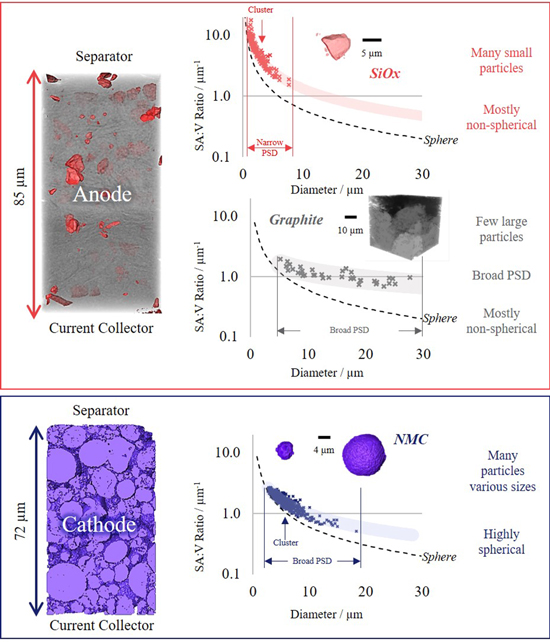
Figure 8. Particle-level data collected from an INR 18540 MJ1 Li-ion cell: top) anode, separated into silicon and graphite, and bottom) cathode, where only NMC is characterized.
Download figure:
Standard image High-resolution imageThe silicon and NMC particles displayed sharp particle size distribution (PSD) peaks around 2 μm and 6 μm, respectively. Whereas the graphite displayed a considerably broader distribution, with peaks between 5–25 μm (Fig. S13). This can be seen by the tight clustering of points for silicon and NMC within Fig. 8, whereas graphite appears disperse without clustering. Although the vast majority of NMC particles fall in the range of 4–10 μm diameters, the PSD is relatively broad with some particles (albeit very few) measuring >15 μm. Nickel-rich NMC (e.g., NMC811) is often reported to have a wider PSD than NMC with lower nickel content (e.g., NMC622),38 and a broad PSD can provide a more efficient packing density; the NMC content within the cathode was found to be approx. 2/3 by volume and this may not be possible without a wide PSD. Additionally, varied particle sizes may also provide versatility with respect to C-rate.39 Consequently, when preparing electrochemical models it is important to examine metrics such as the mass loading (as discussed at the electrode-level) in combination with the full PSD (not only the mean particle size), and if possible, all calculated in 3D to mitigate parallax errors and insufficient statistics.38
Each of the SA:V ratio plots within the figure also display the curve for a perfect sphere as a comparison, providing an indication of sphericity. Sphericity histograms can also be found in the supplementary data (Fig. S13). Although the smaller silicon particles (<3 μm) are relatively spherical, as the particle size increases the degree-of-sphericity declines, producing particle shapes more akin to shards of glass than spheres, with sharp edges and flat surfaces. The sphericity values range from 0.3–0.7, peaking around ∼0.6. Whereas, as observed at the electrode-level, the NMC particles are highly spherical (avg. ∼0.8). The offset from perfect sphericity may be attributed to cracks40 or surface roughness,38 unlike the graphite which displays a sphericity distribution similarly broad to its PSD. The graphite sphericity also appears bimodal (Fig. S13), and through visual inspection of the anode, some graphite particles appear to have been compressed in one plane in the form of an ellipsoid. Advanced shape analysis may provide a more comprehensive understanding of these particles and is an avenue that the authors encourage computational modellers reading this article to pursue using the data from the repository.24
As with most quantifications, many of these metrics can be calculated in different ways, we would, therefore, encourage readers to download the raw data and apply novel segmentation, particle separation, particle orientation, porosity mapping, and other analysis methods.
Discussion
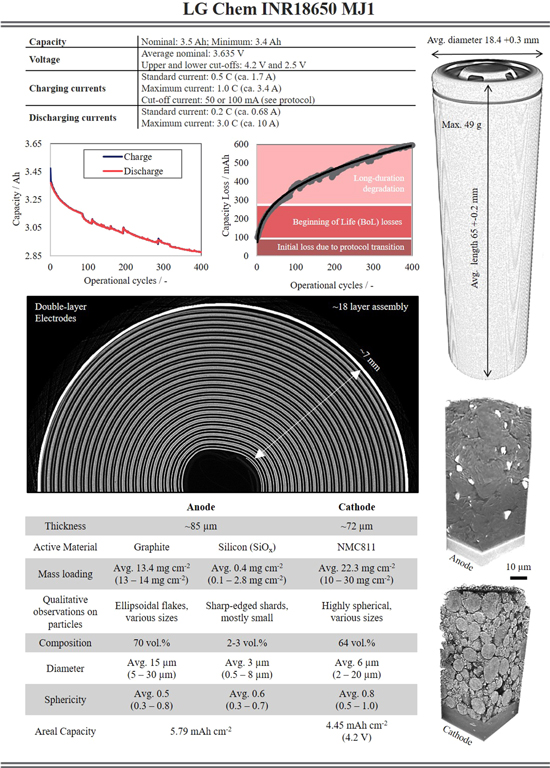
The increasing use of Li-ion batteries has brought a diverse range of cell types within the commercial sector and although certain aspects have been standardized (e.g., geometry) many facets of the cells can vary; particularly, their electrochemical durability (coulombic efficiency and variation in differential capacity), cell chemistry (anode and cathode active material choice and composition), cell assembly (number of cell windings, assembly thickness), electrode make-up (single or double layer, thickness, loading, areal capacity), and finally particle structure (particle diameters, sphericity and surface area to volume ratio). These are just some of the many metrics that may be extracted from a comprehensive electrochemical, chemical and structural analysis. This work has aimed to provide such information and open discussions around other possible analysis that may be carried out. Figure 9 has been produced as a quick-reference guide for the electrochemical and microstructural properties of INR 18650 MJ1 Li-ion cells. Within the figure, key parameters from the manufacturer's electrochemical cycling protocols are outlined, along with the charge and discharge capacities for the first 400 cycles, and the structural features from the full cell assembly, through to the individual particles are quantified. The electrochemical data, 3D full cell, 3D anode and 3D cathode data have all been made freely available to download18 and the authors encourage: further analysis (e.g., novel segmentation, advanced particle shape classification, crack detection and quantification, connectivity, etc.), and modelling (e.g., multi-length scale, time-resolved real-structure, thermal, mechanical, thermal runaway, etc.). Ultimately, through the open-access sharing of comprehensive data packages such as this to the wider research community, we hope to greatly progress our understanding of materials degradation.
Figure 9. An advanced datasheet for INR 18650 MJ1 Li-ion batteries that employ nickel-rich NMC811 cathodes and silicon-graphite anodes.
Download figure:
Standard image High-resolution image
Conclusions
The accelerating development of Li-ion batteries and their increasing uptake in emerging markets such as BEVs has resulted in a diverse range of commercial cell types. This work focusses on a comprehensive electrochemical, chemical and structural analysis of a common cell type: the INR18650 MJ1. This cell was chosen because of its relatively high nominal capacity (3.5 Ah) and electrode chemistries that are of particular commercial and academic interest: silicon-graphite and NMC811.
Within this article, certain regions on the differential capacity profile have been highlighted, with distinction made between mechanisms responsible for capacity loss during the transition between formation and operation cycling protocols (operational cycle 1), fast capacity loss during the BoL cycling (<50 cycles) and more gradual (over hundreds of cycles) long-duration degradation. For instance, the initial onset of charge transfer during charging at low voltage (ca. 3.10 V) was seen to creep to higher voltages with cycling (ca. 3.30 V). Moreover, considerable charging capacity loss was observed after the first cycle and is thought to be attributed the transition between formation and operational discharge C-rates as well as possible gass formation, specifically at low cell potentials (3.55 V). The second two differential capacity peaks around ca. 3.70 V and 4.00 V also developed a reduction in charge transfer; however, less noticeable than the aforementioned losses at lower cell potentials. To accompany the electrochemical characterization, the pristine cell structure has been characterized across several length-scales from the full-cell to the individual particles.
Firstly, the standard cell casing dimensions have been provided in terms of diameter (18.4 mm) and length (65 mm), the number of layers in the electrode assembly quantified: 18 layers ca. 7 mm in total thickness. And the individual components of the assembly characterized: the electrodes are double-layered with approximate thicknesses of 180 μm and 155 μm for the anode and cathode, respectively.
Moving to the electrode level, the individual electrode coating thicknesses were found to be approximately 85 and 73 μm, with a greater variance in the cathode. The anode and cathode areal capacities for operation to 4.2 V were found to be 5.8 and 4.5 mAh cm−2, respectively; the anode has been coated with a higher areal capacity, which is typical of commercial cells. Based upon the limiting capacity (the cathode) and the electrochemical charge capacity, the total electrode area was approximated to be ∼760 cm2.
Assessing each active material in turn allowed for the quantification of metrics from individual particles. The anode was found to contain silicon (avg. 2.2 vol%) and graphite (avg. 70 vol%), whereas the cathode contained only NMC811 (avg. 64 vol%) as the active material. The PSD for the silicon particles was narrow, with small particles that were relatively spherical. However, bigger particles were shard-like in shape with large flat surfaces and sharp edges; whereas the graphite particles had a broader PSD, were considerably larger and consequently fewer in number; the NMC displayed a broad PSD with highly spherical particles, likely in order to optimize packing density and improve C-rate versatility. The loading of the silicon-based material varied considerably throughout the anode, with an average of 0.4 g cm−2 but with some areas exceeding 2.5 g cm−2 locally. Analysis of the oxygen content within Si-material via EDX and X-ray CT (i.e., determining x within SiOx) found a distribution of oxides, where the bulk is likely SiO2 but with sufficient deviation to suggest substantial quantities of pure silicon and other oxides may be present, i.e., it is not a simple binary silicon-carbon compound.
From the information reported within this manuscript and the accompanying raw data within the data repository, the authors envisage several paths for future research. Firstly, novel analysis methodologies may be tested and developed using this as model data, e.g., improved segmentation or crack detection. Secondly, advanced computational modelling may be conducted using the multi-length-scale microstructural data as a boundary mesh; in combination with the electrochemical cycling, the structural developments with operation may be predicted. Additional experimental cycling or modelling would extend the study beyond long-duration through to end-of-life (EoL), e.g., thousands of cycles, for the prediction/observation of cell failure. Thirdly, experiments may be designed around the information here: synchrotron methods may provide greater insight into the oxygen content within the SiOx and operando studies may improve our understanding of these structures during lithiation and delithiation processes.
As new chemistries and commercial cells become available, the authors envisage replicate investigations, whereby the methodology of comprehensively characterizing then releasing the data on a popular cell-type may become common practice. For instance, pouch and prismatic cells are also of interest to both academic and industrial audiences, and may form the basis of future studies. Ultimately, this work produces a baseline of information for readers that will aid many aspects of electrochemical research, from particle-based models to full-scale commercial testing.
Acknowledgments
This work was carried out with funding from the Faraday Institution (faraday.ac.uk; EP/S003053/1), grant number FIRG001 and FIRG003. The authors would like to acknowledge the Royal Academy of Engineering (CiET1718\59) for financial support. Use of the instruments was supported by EP/K005030/1, EP/N032888/1 and EP/M028100/1.
Author contributions
TH and RJ collected the nano-CT data. TH and TT collected the micro-CT data. TH and MK analysed the CT data. AD collected the SEM data. AJ collected all electrochemical data. TH, AJ and CT analysed the electrochemical data. TH, DJL and PRS directed all research. All authors reviewed the article.