
Abstract
The often-observed current distribution between parallel-connected lithium-ion cells within battery modules is probably evoked by the properties of the connection, inhomogeneous contact and power line resistances, the impedance behavior of single cells and of the DoD. The extent to which each of the contributors and the interaction between them affects the current distribution within the battery module is crucial to improve the system's efficiency, which is investigated here via various electrically cross-linked, physicochemical-thermal simulations with variable system terminal (ST). Consequently, cross-connectors balance the system and reduce DoD shifts between cells. Furthermore, if one compares ST-side and ST-cross, the position of the ST is negligible for topologies that incorporate at least two cells in serial and parallel. Depending on the ST configuration, point and axis symmetry patterns appear for the current distribution. Compared to welding seam and cross-connector resistances, the string connector resistance dominates the current distribution. Like the behavior of a single cell, the system's rate capability shows a non-linear decrease with increasing C-rate under constant current discharge. As a recommendation for the assembly of battery modules using multiple lithium-ion cells, the position of the ST is of minor importance compared to the presence of cross-connectors and low-resistance string connectors.
Export citation and abstract BibTeX RIS

This is an open access article distributed under the terms of the Creative Commons Attribution 4.0 License (CC BY, http://creativecommons.org/licenses/by/4.0/), which permits unrestricted reuse of the work in any medium, provided the original work is properly cited.
Range anxiety is named as one of the leading reasons why people buy conventional cars instead of battery electric vehicles (BEVs).1 At same system voltage, an increase in range can be achieved by both higher cell capacities and parallel connection of the cells. As cells with sufficient capacity still lack market maturity, parallel connection is currently the remaining alternative.2 However, parallel connection of cells often leads to inhomogeneous current distributions. An inhomogeneous current distribution can be caused by different reasons. Thus, cell-related causes such as the cell chemistry,2–5 deviations in resistance and capacity,6–12 or different temperature behavior13–16 influence the current distribution. Furthermore, the load profile2,17 and system-related influences such as the connection properties12,18,19 have to be taken into account. Therefore, the focus of this paper is on system-related influences and load profiles.
System-related deviations can be caused by the choice of the system terminal (ST), the internal circuit design of the serial and parallel connection of the cells, or a variation of different contact resistances. Rumpf et al.13 investigated the influence of the ST and found that middle contacting (ST-mid) is preferable to left contacting (ST-left). Grün et al.19 emphasized that the ratio of the cell's internal resistance to the contact resistances is particularly important. Additionally, Wang et al.18 showed that the connector plate causes the current distribution and that their resistance therefore has to be minimized.
So far, only a few researchers have dealt with the general description of interconnected systems. Wu et al.8 developed a semi-experimental equation system to describe serial and parallel connected cells. In contrast to Rumpf et al.13 who described an equation system for ST-side and ST-mid, the influence of the ST on the current deviation was not taken into account. Furthermore, the possibility of inhomogeneous current distribution in parallel-connected cells was neglected by assuming that equal capacities lead to a homogeneous current distribution. For the reader's convenience, additional descriptions of interconnected systems can be found in Refs. 2, 3, 9 and 12.
Even though physicochemical models are becoming more popular due to the advantages of local analyzing opportunities,13,14,16,20 most publications describing serial and parallel connected systems are based on equivalent circuit models (e.g. Refs. 2–4, 15, 21, 22). However, none of the existing publications describe a method of how the ST can be described flexibly or how the connection between serial and parallel strings (cross connectors) can be taken into account.
The focus of this paper is therefore on the development of a system which allows a flexible choice of the ST and considers cross-connectors. For this purpose, the model presented in our previous study13 is developed further and the features named here are implemented. Subsequently, the influence of different STs and varying system resistances on the current distribution within a 4s4p system including cross-connectors is examined. Finally, the energy efficiency of the entire system is evaluated.
Model Structure
The electrical model (ELM) developed by Rumpf et al.13 describes a set of X serial and Y parallel-connected cells and is the basis for the extension presented in this paper. Therefore, the components and the nomenclature of the ELM as well as the coupled simulation model are briefly described. Following that, the extensions of the ELM and the calculation method of the cell currents are discussed. The last part of this section addresses the assumptions made for the simulation.
Basics of the electrical model
The ELM of a 4s4p system including cross-connectors is illustrated in Fig. 1. Additionally, Table I lists all components of the ELM with a short description. Based on their numbering, the components of Fig. 1 can be clearly assigned. As Fig. 1 illustrates, the numbering of the cells corresponds to the numbering of matrix elements. Therefore, the numbering of the cells c starts at the top left with c1,1 and ends at the bottom right with cX,Y. Both the numbering of the cell currents I and the resistances of the welding seams on the positive (Rwsp) and negative (Rwsn) tabs of the cell equal the cell numbering. The connector resistance between two serial cells Rconn gets its number from the cell above it. Rp and Rn are the string connector resistances on the top and bottom between two parallel strings and are therefore numbered according to the string number to their right. The numbering of these string connector resistances ends by Y. If one of the STs is positioned on the right side, the numbering ends by Y + 1. Note that there is no Rconn present at the link between Rwsp and Rp. This is due to the assumption that the tabs are directly welded onto the busbar leading to the ST (see Eq. 6). The same applies to Rwsn and Rn, respectively. The numbering of the cross-connector resistances Rm between two serial-connected cells and two parallel strings is separated from the cell numbering, but also corresponds to the numbering of matrix elements.
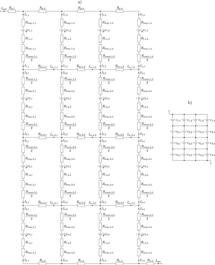
Figure 1. System topology of the ELM for a 4s4p system. Part (a) shows the entire system, including all of its components. Part (b) is the graphically reduced version and will be used instead of (a) in the following. For both versions, the STs are positioned in a cross wise manner. Cross-connectors between adjacent strings and cells resemble a connector plate.
Download figure:
Standard image High-resolution imageTable I. Descriptions, units, and initial values of the components used in the ELM.
| Variable | Initial Value | Unit | Description |
|---|---|---|---|
| φ | 4.2 | V | Voltage of a single cell |
| I | 1 C | A | Current through single cell |
| Iapp |

|
A | Current applied to the system |
| Im | 0 | A | Current through cross-connector m |
| Ri | 28.7 | mΩ | Internal resistance of a single cell |
| Rwsp | 62.5 | μΩ | Resistance of the welding seam at the positive tab |
| Rwsn | 62.5 | μΩ | Resistance of the welding seam at the negative tab |
| Rconn | 30.9 | μΩ | Resistance of the serial connection within a string |
| Rm | 15.4 | μΩ | Resistance of the cross-connector between two strings |
| Rp | 15.4 | μΩ | Resistance of the parallel connection at the positive tab |
| Rn | 15.4 | μΩ | Resistance of the parallel connection at the negative tab |
In order to clarify the naming of the system, in addition to the number of cells connected in serial and in parallel, the location of the ST (left or cross) is also added. Fig. 1 illustrates the system for ST-cross. Furthermore, the system includes four cell packages (I–IV). One cell package includes all cells at the same level of serial connection. For example, cell package III includes the cells c3,1, c3,2, c3,3, and c3,4.
Extension of the electrical model
As shown in Fig. 2, Rumpf et al.13 coupled the ELM with a physicochemical model (PCM) and a thermal model (THM). The coupled model was then used to investigate the influence of the ST, the contact resistance and varying internal resistances, capacities and temperature gradients on the current distribution within parallel-connected lithium iron phosphate (LFP) cells. To calculate the string currents, Kirchhoff's nodal and mesh equations were used and an equation system was given.
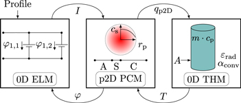
Figure 2. Coupling of the PCM, ELM, and THM according to Rumpf et al.13 An electrical load is applied to the ELM in form of a profile. The shown exchange variables are used to couple the three models.
Download figure:
Standard image High-resolution imageHowever, calculating systems including cross-connectors (see Fig. 1) is not possible with the developed equation system. Additionally, the position of the ST is limited to a side (left or right) and middle connection. Hence, two extensions of the ELM are necessary. First, the model should be capable of dealing with systems including cross-connectors, and second, the position of the ST should be freely chosen.
To ensure that the ST can be freely chosen, setting up the meshes to calculate the string currents has to be considered. Therefore, attention has to be paid to the node where the currents branch differently. Consequently, the sign of affected Rn and Rp has to be adjusted if necessary. The sign of all other components as well as the general calculation method for the currents remains the same as described by Rumpf et al.13
However, including cross-connectors in the ELM has more impact on the calculation algorithm because the mesh equations have to be defined differently. In addition to the increased number of cell currents I, the currents Im through the cross-connector resistances have to be calculated as well. This means that every additional cross-connector adds three additional variables to the equation system. Note that cross-connectors can only be implemented when  holds true. To achieve at least a quadratic equation system, the same number of equations has to be added. Therefore, the procedure of adding equations is explained for a 2s2p system (ST-left), shown in Fig. 3.
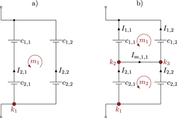
Figure 3. A 2s2p system (a) without and (b) including a cross-connector, highlighting the impact of the cross-connector on the number of currents/equations necessary. In part (a), only two currents are needed to describe the system. In part (b), however, five currents can be distinguished.
Download figure:
Standard image High-resolution imageIn Fig. 3a, only two currents have to be calculated, since the currents through c1,1 and c2,1 as well as through c1,2 and c2,2 are equal. Therefore, two equations are generated by the node k1 on the bottom of string 1 and the mesh m1 in between the cells. This leads to a quadratic equation system that can be solved analytically.
By including the cross-connector in Fig. 3b, three additional currents are generated. Now, the four cell currents I1,1, I1,2, I2,1, and I2,2 as well as the current Im,1,1 through the cross-connector have to be calculated. To do so, the meshes m1 and m2 between c1,1 and c1,2 as well as between c2,1 and c2,2 are determined. Additionally, the node k1 on the bottom of string 1 and the nodes k2 and k3 at the connection points on the left and right of the cross-connector are considered. Consequently, three additional equations are generated and the equation system is analytically solvable. If the system is extended by another cell package in serial or string in parallel, additional resulting nodes and meshes surrounding the additional cross-connectors have to be defined to retrieve the required equations. Consequently, it can be summarized that even in a system including cross-connectors, enough equations can be determined to set up a quadratic equation system.
Specifications of the simulation scenarios
The PCM and THM used in this study are based on the model developed by Sturm et al.23,24 The model development and its parametrization for a nickel-rich manganese cobalt (NMC-811), silicon-graphite (SiC) lithium-ion cell (LG Chem, INR18650-MJ1, 3.35 Ah25), using a wide range of experimental measurements, are shown in detail in Refs. 23, 24. The model equations and the resulting parametrization are summarized in Tables A·I and A·II as well as in Fig. A·1. To maintain the validity of the single cell model the presented simulation studies were chosen within the experimental validated operating range. The single cell PCM shows a mean open-circuit-voltage (OCV) error of 5.7 mV and a mean error of 13.5 mV for 1 C discharge (see Ref. 23, Figs. 1b and 4f). The THM shows a mean temperature error of less than 0.1 K (see Ref. 24, Fig. 4d)) for the intended C-rates. Therefore, it is assumed that the PCM and THM do not significantly affect the results. Furthermore, the following assumptions were made: It is assumed that the subsequently calculated resistances apply to industrially produced, interconnected systems using large format cells. Currently, such systems can be found mainly in BEVs. The available Audi, Jaguar, and Porsche BEVs can be seen as examples.26–28 Additionally, each cell of the system is assumed to have the same capacity, internal resistance, and thermal behavior. Unless stated otherwise, the initial values correspond to those of Table I and the ambient temperature is set to 25 °C. Moreover, the tabs of the cells are considered to be welded onto an aluminum connector plate with a thickness of 2 mm using two 14 mm welding seams on each tab.
Schmidt et al.29 measured a contact resistance of  for Al–Al connections built on a single welding seam with an area of 15.71 mm2. Due to the doubled welding seams, the contact resistance decreases by a factor of 2. Moreover, it is assumed that due to industrialized welding techniques and increased welding areas, the contact resistance can be decreased by an additional factor of 2. In total, the contact resistance of Rwsp and Rwsn is set to 62.5 μΩ. Furthermore, the average distance between the positive and negative tabs lws of the cells connected in serial is assumed to be 3 cm. Additionally, the average distance of adjacent positive or negative tabs is set to be 0.5 · lws. With an electrical conductivity of aluminum of
  ,29 the values of Rconn and Rm can be calculated using Eqs. 1 and 2. Rn and Rp are assumed to have the same characteristics as Rm and are therefore set to the same value (Eq. 3).

A common feature of the BEVs mentioned here is the use of large format lithium-ion batteries with a capacity of approx. 60 Ah. In order to ensure practical relevance, a capacity of 60 Ah is therefore assumed to be the reference cell capacity in the following. However, the model developed by Sturm et al.23 was validated for a 3.35 Ah cell. As the cell under consideration and the cell used by Sturm et al.23 differ in capacity and resistance, the values of Rwsp, Rwsn, Rconn, Rm, Rp, and Rn from Table I have to be scaled to ensure comparability. Therefore, a scaling factor scaling factor SF has to be calculated, using the ratios of the cells' capacities or internal resistances. Since the focus of this study is not on high power but on high energy applications, the influence of the capacity should dominate the influence of the resistances. Consequently, the initial values of the resistances named here are scaled by the cells' capacities using  .
.
Subsequently, the influence of different STs, varying Rwsp, Rm, and Rp on the current distribution is discussed. Therefore, a side (ST-left) and cross-connection (ST-cross) are investigated first. Following this, the influence of varying Rwsp are examined. The value of the homogeneous case is therefore increased by +100%. Next, the same variation is applied to different Rm. Finally, the rate capability of the extractable energy content of the system is examined. Note that only one Rwsp, Rm, or Rp is varied at a time. Table II summarizes the investigated cases. Note that Rumpf et al.13 showed that middle contacting would lead to a more homogeneous current distribution. Consequently, the deviations shown in the following exceed the deviations of middle contacting, which is why the focus of the following investigations is on ST-left and ST-cross.
Table II. Overview of the investigated cases.
| Investigation | Initial Value | Variation |
|---|---|---|
| ST | —– | left, cross |
| Rwsp | 62.5 μΩ | +100% |
| Rm | 15.4 μΩ | +100% |
| Rp | 15.4 μΩ | +100% |
| Iapp | 1 C per cell | C-rate |
As described above, it is assumed that every cell has the same thermal behavior. Consequently, the conditions (see Tables A·I and A·II) applied to the cells are equal. Furthermore, thermal coupling between adjacent cells as well as heat transfer through contact surfaces have not yet been implemented in the THM. Therefore, an equal current load leads to an equal temperature behavior, independently of a cell's position within the system. As shown below, the current distribution throughout the system exhibits relatively small deviations between cells over a wide depth of discharge (DoD) range. Consequently, uneven temperature development is not expected to have a significant influence on the current deviation for the investigated cases. However, the development of a thermally coupled model and the analysis of temperature gradients and cooling strategies within battery systems are crucial for cooling strategies and battery safety and may be the scope of future studies.
The applied current to the system equals Y · I1C. That in turn means that the expected current load per cell is equal to a C-rate of  (I1C). Each discharge begins with fully charged cells (DoD = 0) at a cell voltage of 4.2 V and ends when a cell reaches the discharge cutoff voltage of 2.5 V (DoD = 1). This means that for the investigated 4s4p system the measurable voltage level at the STs is between 16.8 V and 10.0 V. Furthermore, the expected amount of energy that can be drawn from the system equals the sum of the extractable energies of the individual cells and can be calculated using the following equation:

In this matter, the nominal energy (EN,sys) is summarized from the total of all cells ( ), which is used to compare the simulated cases shown in Table II.
Results
The following results are based on the systems 4s4p ST-left and 4s4p ST-cross, as described above. Both systems include cross-connectors.
Influence of the system terminal
Figure 4 illustrates the resulting current distribution of a 4s4p system connected on the left side (ST-left, (a)) and cross-connected (ST-cross, (b)), for the homogeneous case. Homogeneous here means that the same system components have the same initial values. By comparing Figs. 4a and 4b qualitatively, it can be seen that there is no difference between the current distribution within the systems. Note that equal line colors indicate quasi-identical current distributions of different cells within the systems. Therefore, it can be stated that within XsYp systems including cross-connectors, the choice of the ST is negligible for the homogeneous case, if  holds true.
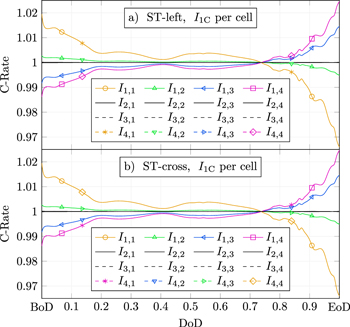
Figure 4. Influence of the STs on the current distribution in the homogeneous case for a 4s4p system including cross-connectors. The system in (a) is contacted on its left side (ST-left), the system in (b) is cross-connected (ST-cross).
Download figure:
Standard image High-resolution imageAdditionally, five current paths can be distinguished in both subplots. As a total of 16 current distributions have to occur for the analyzed 4s4p system, the noticeable current paths can be interpreted as group current paths. It is therefore necessary to clarify where the number of group paths originates from and how the groups are formed.
Considering Fig. 4, the number of group paths strongly depends on the number of cells connected in parallel, since a group current path occurs for each of the  parallel strings. These current paths differ from the applied current of I1C for the first and the last cell package of the system due to uneven path resistances RPR.2,13 For parallel-connected systems with
  , an additional group current path occurs which lies directly on the applied current line. Consequently, the number of group current paths
  within a XsYp system is given by the following rule:

Marking the cells from the same group current path in Fig. 1b leads to Fig. 5. Considering ST-left shown in Fig. 5a, the current distribution within the system follows the axis symmetry to the mirror axis between cell packages II and III. On the other hand, the current distribution regarding ST-cross leads to point symmetry to the central point of the system of Fig. 5b. Once again, the symmetries can be justified with the cells' RPR. For example in the case of ST-cross RPR of c1,3 and c4,2 to the nearest ST calculate to:


Figure 5. Resulting symmetry for homogeneous interconnected systems. Side connection (a) leads to axis symmetry, cross-connection (b) leads to point symmetry. As in Fig. 1, the numbers stand for the cell index. Colors and letters both highlight the symmetry and thus mark symmetry partners.
Download figure:
Standard image High-resolution imageSince Eqs. 6 and 7 consist of equal system elements with equal values, the same current is applied to c1,3 and c4,2.
The symmetry effects found can now be used to examine the maximum deviations from the applied current at the beginning of discharge (BoD) and at the end of discharge (EoD) (see Fig. 4). Note that the choice made for BoD and EoD represents the maximum deviation during the entire discharge of the cells, as can be seen in Fig. 4. This is why the deviations from the applied current at these points in time can be assumed to be a worst-case scenario. Table III lists the deviations from the applied I1C discharge current for cells c1,1, c1,2, c1,3 and c1,4 for the homogeneous case.
Table III. Maximum deviation to the applied I1C current at the beginning (BoD) and at the end of discharge (EoD). The same deviations apply to the symmetry partners of the cells according to Fig. 5.

|

|

|

|
|
|---|---|---|---|---|
| BoD |

|

|

|

|
| EoD |

|

|

|

|
Thus, at the beginning, I1,1 and I1,2 are increased by 1.9% and 0.3% due to their smaller RPR as compared to the applied I1C current. In contrast, I1,3 and I1,4 are decreased by 0.8% and 1.4%. Consequently, until currents cross at around 75% DoD, c1,1 and c1,2 are discharged with a higher current and their DoD increases faster. Subsequently, c1,3 and c1,4 have to compensate for this imbalance until the EoD. Therefore, I1,3 and I1,4 increase up to 1.5% and 2.4% compared to the applied I1C current. Depending on the choice of the ST, these deviations correspond to the deviations of the symmetry partners marked in Fig. 5. Cells of cell packages II and III are not listed because their maximum deviation to the applied I1C current is less than 0.02% and is therefore considered negligible. Furthermore, an extractable energy content for the homogeneous case Ehom of 193.2 Wh occurs for both systems. Since the nominal energy content of a single cell calculates to  , following Eq. 4 EN,sys calculates to 194.9 Wh. Consequently, 99.13% of EN,sys can be extracted for the homogeneous case.
The analysis by Hofmann et al.,3 performed with an equivalent circuit model using linearized OCV, showed that differences in OCV, impedance, and capacity are the main reasons for an inhomogeneous current distribution within parallel connections. Thereby, differences in the OCV dominate the influences of uneven capacity and impedance. To further analyze the origin of the current distribution, the PCM was used to perform a polarization analysis.30 With respect to the complexity, the analysis was conducted for the upper cell package in Fig. 3b instead of a cell package of the 4s4p system. The parametrization of the PCM, ELM, and THM remained unchanged (see Table II). Figure 6 illustrates the resulting differences in polarization and OCV between the cells. Since RPR,1,1 is decreased as compared to RPR,1,2, c1,1 is discharged with an increased current compared to c1,2 at the BoD. Since the polarization of the single cell depends on the current, the resulting inhomogeneous current distribution causes a difference in the polarization of c1,1 and c1,2. In addition, as both cells are discharged from 0% DoD, no OCV shift occurs at the BoD. Hence, the current distribution is caused by the differences in RPR and polarization during the BoD. However, with progressive discharge of the cells, the inhomogeneous current distribution leads to a difference of the cells' DoDs. As a result, the cells' OCVs are shifted against each other. Figure 6 also illustrates that as soon as the difference of the OCVs exceeds the difference of the polarizations, the shift of the cells' OCVs becomes dominant. As the OCV difference leads to different cell potentials, the current distribution is dominated by the OCV difference. For the modeling design, this means that the use of a validated equivalent circuit model could also be justified. However, since the polarization analysis is seen as an important tool for subsequent studies, a PCM model was also used for the sensitivity analysis shown in the following. Note that Fig. 6 does not include differences of the polarization at surrounding components, and thus the difference between the cells' OCVs and the internal polarizations η differs from zero.

Figure 6. Analysis of the differences in polarization and OCV for cells c1,1 and c1,2 of the homogeneous 2s2p system of Fig. 3b for a 1 C discharge. The difference Δ indicates the difference between cell c1,2 and c1,1, i.e.  . Differences in the polarization at surrounding components are not included in the diagram.
Download figure:
Standard image High-resolution imageInfluence of the welding seam resistance
The influence of Rwsp on the current deviation within both systems is analyzed next. For this purpose, all Rwsp are successively increased by +100% for ST-left and ST-cross.
Figure 7 illustrates an example of the resulting current profile of the 4s4p system (ST-left) for a variation of Rwsp,1,1 as compared to the homogeneous case. Due to the increased contact resistance of c1,1, I1,1 decreases in the beginning. At the same time, I1,2, I1,3, and I1,4 have to increase so that cell package I can still pass on the required current to the next cell package level (II). Consequently, the increased current through cells c1,2, c1,3, and c1,4 at the BoD leads to a faster discharge of these cells. This in turn means that at the EoD, c1,1 has to deliver a higher current as compared to the homogeneous case, whereas the currents through c1,2, c1,3, and c1,4 decrease. This means that there is always an interplay of the current load within the cell package so that the overall applied current of 4 · I1C can be passed on to the next cell package. Hence it is examined next, if a variation of Rwsp only affects cells within the same cell package and therefore, whether every cell package can be analyzed independently.
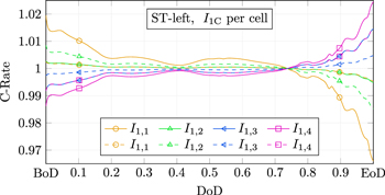
Figure 7. Influence of the variation of Rwsp,1,1 (dashed lines) on the current distribution within cell package I as compared to the homogeneous case (solid lines).
Download figure:
Standard image High-resolution imageAccordingly, Fig. 8 illustrates the deviations of the cell currents at the EoD (see Fig. 7) as compared to the applied I1C current for a variation of Rwsp. On the left side of Fig. 8, every subplot illustrates the influence of Rwsp on the current deviation of the symmetry partners for ST-left. Consequently, the influence of Rwsp,1,1 on the currents of cell package I can be investigated by comparing the deviation of I1,1, I1,2, I1,3, and I1,4 in the subplots (a), (b), (c), and (d) (dotted lines) above index 1,1. In contrast, if a variation of Rwsp,1,1 would affect cell currents of cell packages II, III, or IV, at least one cell current of I2,1, I3,1, I4,1, I4,2, I4,3, or I4,4 would deviate from the homogeneous case (index h) under variation of Rwsp,1,1 (index 1,1) in Fig. 8. As this is not the case, it can be stated that a variation of Rwsp,1,1 only affects cell currents within cell package I. If one continues to analyze the effects of the variations in other Rwsp (index 1,2 − 4,4), this statement by cell package I can be extended to the entire system. Accordingly, it can generally be stated that an increased contact resistance only affects the cell package in which the increased contact resistance occurs. Thus, each cell package can be evaluated in a decoupled manner. The reason why a variation within a cell package has no influence on the surrounding cell packages is the presence of cross-connectors between the cell packages. Consequently, cross-connectors can be seen as balancing elements inside the system.
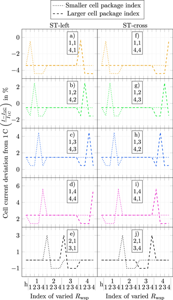
Figure 8. Influence of varying Rwsp on the current distribution within interconnected 4s4p systems. Each subplot illustrates the current deviation from I1C for the symmetry partners of the cell package with the smaller (dotted) and larger (dashed) index at the EoD. The x-axis refers to the varied (+100%) Rwsp, whereas h represents the homogenous case. Consequently, the influence of the varied Rwsp on the cell of interest can be seen in the related subplot.
Download figure:
Standard image High-resolution imageDue to the finding that cell packages can be analyzed individually, the position of an increased Rwsp within the cell package is investigated further. Hence, a variation of Rwsp,1,1, Rwsp,1,2, Rwsp,1,3, or Rwsp,1,4 leads to a maximum increase at the EoD of the currents I1,1, I1,2, I1,3 or I1,4, of 2.94%, 2.98%, 3.01%, or 3.04% as compared to the homogeneous case. Referring to the symmetry partners shown in Fig. 5, the same deviations occur for a variation of Rwsp within cell package IV. Within cell packages II and III, a deviation of 3.01% as compared to the homogeneous case remains the same for every varied Rwsp, as indicated by the subplots (e) and (j) in Fig. 8. The maximum difference between the deviations of all investigated cases can be calculated to 0.1%. Consequently, the influence of the position of an increased Rwsp has no significant impact on the rate of current increase for the analyzed system. The reason for this is that the ratio between Rwsp to the resistance of Rm and Rp is dominated by the welding seam resistances. An increase of Rwsp reinforces this effect, which is why the named resistances are even less important.
Additionally, the impact of Rn, Rp, Rm, and Rconn on the maximum cell current load can be examined by evaluating the deviation at the EoD as compared to the applied I1C current rate. Thus, I1,1, I1,2, I1,3, and I1,4 deviate at the EoD from the applied I1C current in the homogeneous case by  ,
,  , 1.46%, and 2.45%, and under variation of the corresponding Rwsp by
  , 2.48%, 4.48%, and 5.50% (see Fig. 8). Therefore, it can be determined that in both cases, the maximum cell current load increases with increasing distance to the ST for cell package I. This can in turn be explained by the fact that an increased distance from the ST corresponds to an increased RPR, which leads to a lower current load during the BoD and an increased current load during the EoD (see also Fig. 7). As described above, an increase of Rwsp reinforces this effect. Therefore, it can be summarized that the position of an increased Rwsp has no impact on the rate of current increase within the cell package, but on the maximum current deviation at the EoD.
Varying Rwsp within a 4s4p ST-cross system leads to the results in Figs. 8f–8j. Compared to the results of ST-left, only the symmetry partners change according to Fig. 5b for ST-cross. The aforementioned conclusions apply similarly for the cross-connected system. That also holds true for the influence of the position and the rate of current increase that corresponds to the variation of Rwsp.
Furthermore, only a negligible influence of a variation of Rwsp on the extractable energy content can be observed, as the difference between the maximum and the minimum extractable energy only calculates to 0.01 Wh. This in turn means that an increased Rwsp by  could not be detected by the measurable extractable energy content at the system terminals.
Influence of the cross-connector resistance
In addition to the influence of Rwsp, the influence of increased Rm on the current distribution is investigated next. For this reason, Rm were increased individually by  for both system configurations. Table IV evaluates the maximum current deviation of Im as compared to the homogeneous case under variation of Rm. Therefore, it can be seen that Rm,1,2 and Rm,3,2 show the highest current deviation of
  . This current is distributed to the subsequent cell package differently than in the homogeneous case. Moreover, in the worst case,
  is passed on to only a single cell of the next cell package over the entire I1C discharge. Compared to I1C, an additional deviation of
  corresponds to a current of 0.024% of the cells' current. Such a deviation is therefore classified as not significant. Furthermore, the extractable energy content under a variation of Rm equals the value of the homogeneous case. Accordingly, it can be said that an increase of Rm by
  has no significant influence on either the current distribution or the extractable energy content of the analyzed system.
Table IV.
Maximum current deviation of Im as compared to the homogeneous case under variation of Rm by  . The entries marked with * have a maximum deviation of less than 3 · 10−6% and were therefore set to zero.
| Rm,1,1 | 0.016% | Rm,1,2 | 0.024% | Rm,1,3 | 0.011% |
| Rm,2,1 |

|
Rm,2,2 |

|
Rm,2,3 |

|
| Rm,3,1 | 0.016% | Rm,3,2 | 0.024% | Rm,3,3 | 0.011% |
Taking into account the respective symmetry partner, Table IV and the statements made apply equivalently to ST-cross.
Influence of the string connector resistance
After investigating the influence of Rwsp and Rm, the influence of varying string connectors is examined next. Therefore, Rp,2, Rp,3, and Rp,4 of cell package I are successively increased by  for both systems. A variation of Rn,2, Rn,3, and Rn,4 is omitted, due to symmetry effects to cell package I.
Figure 9 illustrates the current distribution within cell package I for a variation of Rp,2 in a system with ST-left. Compared to the homogeneous case, I1,1 is increased by 1.3% at the BoD whereas I1,2, I1,3, and I1,4 are decreased by 0.5%, 0.4% and 0.4%. The reason for this deviation is that the string connectors can be seen as segmenting elements of the system. The segmenting in turn leads to increased RPR for all strings, whose position in the current path is behind the varied resistance. Consequently, strings with higher RPR lead to lower string currents at the BoD, and thus I1,2, I1,3, and I1,4 are decreased during the BoD and only I1,1 is increased. Consequently, if Rp,2 is increased, cell package I divides into two segments. String 1 is located in front of the increased string connector and experiences a higher current during the BoD because of the lower path resistance. However, if Rp,3 is varied, the deviation of I1,1 and I1,2 is smaller, since the additional current can split up to both strings. In contrast to Rp,2 and Rp,3, Rp,4 takes a special place, as it is the last string connector. Figure 1 illustrates that Rp,4 acts as an element of the string itself rather than as a string connector. Thus, a variation of Rp,4 leads to the same findings as varying Rwsp,1,4.
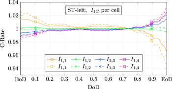
Figure 9. Influence of the variation of Rp,2 (dashed lines) on the current distribution within cell package I as compared to the homogeneous case (solid lines). The result is independent of the ST.
Download figure:
Standard image High-resolution imageComparing the maximum current deviations occurring for a variation of Rwsp (see Fig. 8) to those of a variation of Rp, the influence of varying Rwsp seems to dominate Rp's influence. However, taking into account that there is a factor of 4 between the increased values of Rp and Rwsp and only a factor of 1.7 between the maximum deviations at the EoD, it can be determined that the influence of Rp dominates the influence of Rwsp on the current distribution within the system. The same applies for Rm, since, as shown above, the influence of a variation of Rm is negligible. Consequently, it can be stated that attention has to be paid to the string connectors when assembling such a system.
The maximum deviation of the extractable energy from the homogeneous case calculates to 0.02 Wh for a variation of Rp. Thus, even an increased string connector resistance cannot be detected by means of the measurable extractable energy content. This in turn means that none of the investigated cases can be detected due to measurable quantities at the STs. The almost constant extractable energy is thus achieved by a higher load on individual system components (see deviations in Fig. 9). The impact of this effect on the durability of the components and thus of the investigated system therefore needs to be investigated in further studies.
Rate capability and energy efficiency of the system
Previous sections have shown that the influences of varying Rwsp, Rm, and Rp on the current deviation and the extractable energy content of the system is negligible for a 1 C constant-current discharge. Therefore, the influence of various C-rates is investigated to demonstrate both the rate capability and the influence of varying contact resistances on the extractable energy content of the system. For this purpose, various C-rates (1, 1.25, 1.5, 1.75, 2, 2.25, 2.5, 2.75, and 3) were applied to a 4s4p system connected on the left (ST-left). Additionally, a variation of Rp,2 by  was accomplished to examine whether the extractable energy content differs significantly from the homogeneous case. As it is assumed that the analysis of the extractable energy content is more meaningful for the rate capability of the system than the maximum current deviation at a specific point in time, the following analysis focuses on the extractable energy content. Since the previous sections have shown that the variations of Rwsp and Rm have a minor influence compared to Rp, an additional analysis of the variation of Rwsp and Rm is omitted here. Furthermore, an additional analysis of ST-cross was not conducted due to the symmetry effects shown in Fig. 5.
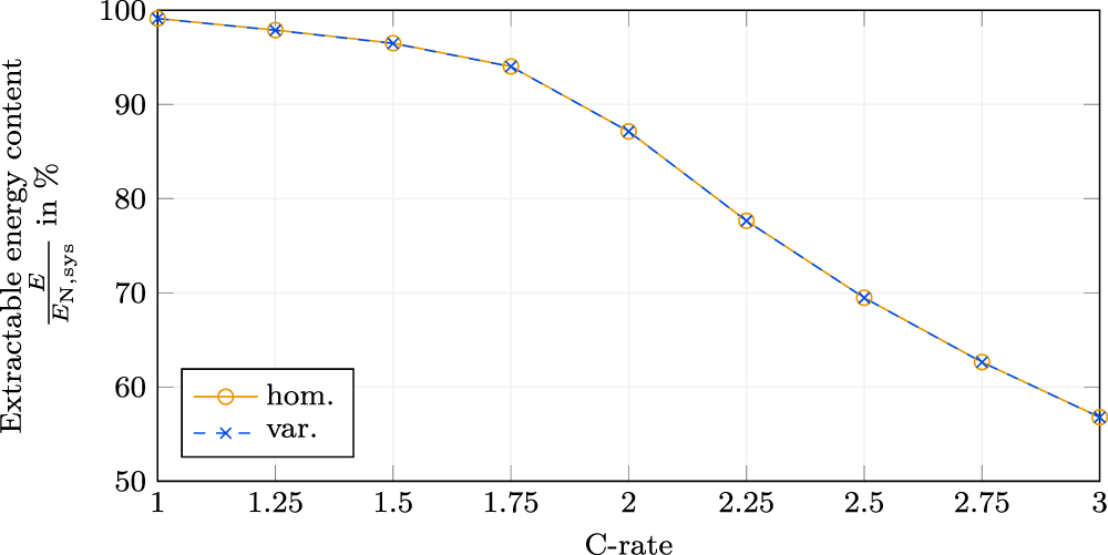
Figure 10 illustrates the extractable energy content for the homogenous case (solid line) and for a variation of Rp,2 (dashed line) for the C-rates named above. Comparing the homogeneous and varied cases, significant deviation of the extractable energy content cannot be depicted, since the maximum deviation calculates to 0.03%. Furthermore, the rate capability of the extractable energy content can be divided into two branches. The first one is represented by the range of 1 C to 1.75 C. In this domain, the extractable energy content decreases from 99.1% (1 C) to 94.5% (1.75 C) for both cases, which equals a mean decrease of 1.53% per increase of C-rate by 0.25 C. Within the second branch, the mean gradient of energy content per increase of the C-rate by 0.25 increases to 7.54% in the remaining range between 1.75 C and 3 C. This results in an extractable energy content of 56.8% for an applied 3 C-rate.
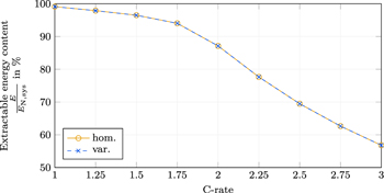
Figure 10. Extractable energy content of the analyzed 4s4p system for different C-rates. Solid lines show the amount in the homogeneous case, dashed lines refer to an increase of Rp,2 by  .
.
Download figure:
Standard image High-resolution imageConsequently, the analysis clearly shows the trend of a decreasing rate capability of the extractable energy content with increasing C-rates. Furthermore, the findings show that an increased contact resistance leads to a more uneven current distribution, but that the extractable energy content remains the same. This leads to the assumption that the almost constant energy output is achieved by higher loads on individual system components, which is why the longevity has to be investigated further. In addition, for future studies the cell parametrization can be further specified in subsequent steps, as shown by Mao et al.31 and Rheinfeld et al.32 These extensions would take into account additional limitations of electrode kinetics, and thus increase the accuracy of the p2D model in the event of even higher C-rates, especially higher than 3 C. Table V summarizes the results of the investigated cases.
Table V. Summary of the investigated cases.
| Investigation | Initial Value | Variation | Critical Component | Result |
|---|---|---|---|---|
| ST | — | left, cross | cross-connectors | both 
|
| axis and point symmetry | ||||
| Rwsp | 62.5 μΩ | +100% |

|

|
| Rm | 15.4 μΩ | +100% |

|

|
| Rp | 15.4 μΩ | +100% |

|

|
| iapp | 1 C per cell | C-rate |
 (3 C) (3 C) |
Conclusions
In this study, the structure of the ELM which describes battery cells connected in serial and in parallel as described in Ref. 13 is extended to include flexible STs and cross-connectors. Based on this extension, the influence of ST-left and ST-cross, as well as the influence of the welding seam resistance, the cross-connector resistance and the string connector resistance on the current distribution within a 4s4p system including cross connectors are examined. Finally, the rate capability and the energy efficiency of the systems are investigated for different C-rates.
If cross-connectors are implemented in the system, the choice of the ST is negligible. Moreover, depending on the choice of the ST, symmetries can be found within the analyzed system. Thus, ST-side leads to axis symmetry to the middle axis of the system, whereas ST-cross leads to point symmetry to the system's center point. For the homogeneous case, the maximum current deviations within the analyzed system could be found at the BoD and at the EoD with a maximum deviation of 1.9% and 2.4%, respectively. With increasing distance to the ST, the current deviation decreases at the BoD, but increases at the EoD. These deviations occur in cell packages I and IV, whereas the deviation within cell packages II and III is nearly zero and therefore negligible.
Furthermore, an increased welding seam resistance by 100% alters the current distribution of all cells in the respective cell package, but does not affect other cell packages within the system. This is due to the presence of cross-connectors, which is why cross-connectors can be seen as balancing elements. Additionally, an increase of a cross-connector resistance by 100% has no significant influence on the current distribution within the system. If the maximum deviations of the cell packages are compared with one another, a variation of a welding seam resistance on one of the enclosed cell packages II and III shows the greatest influence.
Moreover, the variation of the string connector resistances by 100% showed that the influence of the string connectors on the current distribution dominates the influence of the welding seam resistance. Thus, particular attention should be paid to the assembling process. Additionally, the investigation showed that string connectors can be seen as segmenting elements of the system.
The extractable energy content of the investigated system remained almost the same for all examined cases performed with a constant current discharge of 1 C. This in turn means that the measurable energy content cannot be used as an indicator for inhomogeneous welding seam resistances, cross-connector resistances, or string connector resistances within the system.
Finally, the investigation of the rate capability of the system showed that the extractable energy content decreases non-linearly with the C-rate. Furthermore, the extractable energy content under a variation of a string connector resistance remained almost the same as compared to the homogeneous case. This in turn means that the nearly constant output is achieved by higher load on individual system components, and thus the long-term durability has to be investigated further.
Future studies should therefore verify these results using measurement data. In particular, the heat input into the cells resulting from increased resistances as well as temperature gradients in general should be analyzed. Further extensions of the model could take into account additional limitations of electrode kinetics to improve the model's high current behavior. Furthermore, the influence of inhomogeneous current distribution on the aging behavior of parallel-connected cells should also be investigated.
Acknowledgments
The results presented were achieved in association with an INI.TUM project, funded by the AUDI AG. Additionally, this work has received funding from the European Union's Horizon 2020 research and innovation programme under the grant 'Electric Vehicle Enhanced Range, Lifetime And Safety Through INGenious battery management' [EVERLASTING-713771].
: Appendix. Model Characteristics
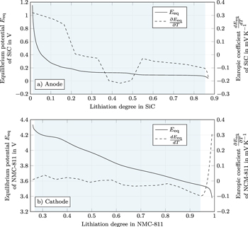
Figure A·1. Characteristics of the investigated cell. (a) and (b) illustrate the Eeq and entropic coefficient  of anode and cathode. The highlighted areas correspond to the usable voltage window.
Download figure:
Standard image High-resolution imageTable A·I. Equations for the single p2D model.
| Electrochemical-thermal model (single p2D) | |
|---|---|
| Mass balance I |
|
|
|
| Potentials I |

|

|
|
| Charge balance I |

|
| Electrode Kinetics I |
![${j}_{n}(x,t)=\tfrac{{i}_{0}(x,t)}{F}\left[\exp \left(\tfrac{{\alpha }_{{\rm{a}}}\,F\,\eta (x,t)}{R\,T}\right)-\exp \left(-\tfrac{{\alpha }_{{\rm{c}}}\,F\,\eta (x,t)}{R\,T}\right)\right]$](https://content.cld.iop.org/journals/1945-7111/167/12/120542/revision2/jesabad6bieqn56.gif)
|

|
|

|
|
| Temperature I,II |

|
| Heat sources |
|
|
|
|
|

|
|
|
|

|
|

|
|

|
|
![$x\in [0,{L}_{\mathrm{neg}}]\wedge [{L}_{\mathrm{neg}}+{L}_{\mathrm{sep}},{L}_{\mathrm{neg}}+{L}_{\mathrm{sep}}+{L}_{\mathrm{pos}}]$](https://content.cld.iop.org/journals/1945-7111/167/12/120542/revision2/jesabad6bieqn68.gif)
Table A·II. Parameterization of the single p2D model with NMC-811/SiC electrodes.
| Geometry | Silicon-graphite | Separator | Nickel-rich | |
|---|---|---|---|---|
| (SiC) | NMC-811 | |||
| Thickness L | 86.7 μm m | 12 μm m | 66.2 μm m | |
| Particle radius rp | 6.1 μm m,D50 | 3.8 μm m,D50 | ||
| Active material fraction εs | 69.4% e | 74.5% e | ||
| Inactive fraction εs,na | 9% e,* | 8.4% e,* | ||
| Porosity εl | 21.6% m | 45% e | 17.1% m | |
| Bruggeman coefficient β V II,** | 1.5 | 1.5 | 1.85 e | |
| Thermodynamics | ||||
| Equilibrium potential Eeq | see Fig. A·1a m | see Fig. A·1b m | ||
Entropic coefficient 
|
see Fig. A·1a m | see Fig. A·1b m | ||
| Stoichiometry | 100% SoC | 0.852 | 0.222 | |
| 0% SoC | 0.002 | 0.942 | ||
| Max. theoretical loading bg | 415 mAh g−1 I | 275.5 mAh g−1 II | ||
| Density ρ | 2.24 g cm−3 I | 4.87 g cm−3 II | ||
| Concentration cs,max | 34684 mol m−3 e | 50060 mol m−3 e | ||
| Transport | ||||
| Solid diffusivity Ds *** | 5 · 10−14 m2 s−1 e,V | 5 · 10−13 m2 s−1 IV,VI | ||
Specific activation  *** *** |
1200 K e | 1200 K e | ||
| Solid conductivity σs | 100 S m−1 IV | 0.17 S m−1 e,IV | ||
| Film resistance Rf | 0.0035 Ω m2 III | 0 Ω m2 e | ||
| Kinetics | ||||
| Reaction rate constant k *** | 3 · 10−11 m s−1 e | 1 · 10−11 m s−1 e | ||
Specific activation  *** *** |
3600 K e | 3600 K e | ||
| Transfer coefficient αa/c | 0.5 e | 0.5 e | ||
m = measured e = estimated * PVDF binder/Carbon black (Refs. 35, 36).
I Ref. 37. II Ref. 38 III Ref. 31 IV Ref. 39 V Ref. 40 VI Ref. 41 VII Ref. 42.
** Effective transport correction according to Bruggeman (Ref. 42):  .
.
*** Arrhenius law (Ref. 43): ![$i(T)=i\cdot \exp \left(\tfrac{{E}_{{\rm{a}},i}}{R}\tfrac{(T-298[{\rm{K}}])}{T\cdot 298[{\rm{K}}]}\right)\,\mathrm{with}\,i\in k\wedge {D}_{s}$](https://content.cld.iop.org/journals/1945-7111/167/12/120542/revision2/jesabad6bieqn73.gif) .
.
Table A·III. Nomenclature
| Greek symbols | ||
|---|---|---|
| Symbol | Unit | Description |
| α | Transfer coefficient | |
| αconv | W m−2 K−1 | Heat transfer coefficient |
| β | Bruggeman coefficient | |
| ε | Volume fraction | |
| εrad | Radiation emission coefficient | |
| η |

|
Overpotential |
| κ |

|
Ionic conductivity |
| ρ | kg m−3 | Mass density |
| σ |

|
Electrical conductivity |
| σB | 5.67 · 10−8 W m−2 K−4 | Stefan-Boltzmann constant |
| φ |

|
External cell potential between cell terminals |
| Φ |

|
Internal electrical potential |
| Latin symbols | ||
|---|---|---|
| Symbol | Unit | Description |
| a | m−1 | Specific surface |
| A | m2 | Surface area |
| A | Anode (domain) | |
| c | mol m−3 | Concentration of lithium cations ( ) ) |

|
mol m−3 | Maximum theoretical concentration of 
|
| ci | Cell under consideration | |

|
J kg−1 K−1 | Heat capacity |
| C | Cathode (domain) | |
| D | m2 s−1 | Diffusion coefficient |

|

|
Equilibrium potential vs 
|

|
Wh | Extractable system energy content for the homogeneous case |

|
Wh | Nominal cell energy content |

|
Wh | Nominal system energy content |

|
Wh | Extractable system energy content |

|
Mean molar activity coefficient of electrolyte | |
| F | 96 485 A s mol−1 | Faraday's constant |
| i | A m−2 | Current density |
| Ii |

|
Current through single cell |

|

|
Current applied to the system |

|

|
Current applied to the cell equals 1 C |

|

|
Current applied to the cell equals 3 C |
| Im |

|
Current through cross-connector |
| i0 | A m−2 | Exchange current density |
| jn | mol m−2 s−1 | Pore-wall flux |
| k | m s−1 | Reaction rate constant |

|
Current node (Kirchhoff) | |

|
m | Length of welding seam |
| L | m | Thickness |
| m | kg | Mass of the jelly roll |

|
Mesh (Kirchhoff) | |

|
Number of group current paths | |
| r | m | Radial coordinate in active particles of p2D model |

|
m | Particle radius |
| R | 8.314 J mol−1 K−1 | Gas constant |

|
Ωm2 | Internal heat resistance |
| RP | m | Particle radius |

|
Ω | Resistance of the serial connection within a string |

|
Ω | Film resistance |

|
Ω | Internal Resistance |

|
Ω | Cross-connector resistance |

|
Ω | String connector resistance (negative tab) |

|
Ω | String connector resistance (positive tab) |

|
Ω | Path resistance |

|
Ω | Welding seam resistance (negative tab) |

|
Ω | Welding seam resistance (positive tab) |
| S | Separator (domain) | |
| ST | System terminal | |
| SF | Scaling factor | |
| q | W m−2 | Heat generation rate per area |
| Q | W | Heat generation rate |

|
W | Internal heat |
| t | s | Time |
| T | K | Temperature |

|
Transport number of 
|
|
| x | x-coordinate in p2D model | |
| X | Number of cells connected in serial | |
| Y | Number of cells connected in parallel | |
| Indices | ||
| Symbol | Description | |
| a | Anodic reaction (oxidation) | |
| c | Cathodic reaction (reduction) | |
| conv | Heat convection | |
| eff | Transport corrected (Bruggeman correlation) | |
| l | Liquid phase (i.e. electrolyte) | |
| neg | Negative electrode | |
| pos | Positive electrode | |
| rad | Heat radiation | |
| r | Reaction heat | |
| rev | Reversible heat | |
| s | Solid phase (i.e. active particle) | |
| sep | Separator | |
| ss | Active particle surface in solid phase | |
| surf | Surface | |