Crawling the cosmic network: exploring the morphology of structure in the galaxy distribution

Abstract

1 INTRODUCTION

Inflationary models of the early universe (Guth 1981) suggest that the large-scale distribution of matter should be well described by a Gaussian random field, the statistical properties of which can be completely specified by the power spectrum. As structure evolves, however, non-linear effects become increasingly important and higher-order statistics must be computed if we wish our description to be complete. A number of studies have been performed to measure the three-point correlation function of galaxies (e.g. Peebles & Groth 1975; Gaztanaga & Frieman 1994; Kulkarni et al. 2007; Nichol et al. 2007) and its Fourier Transform (the bispectrum), as well as N-point statistics (e.g. Fry & Gaztanaga 1993; Verde, Heavens & Matarrese 2000; Ross, Brunner & Myers 2007). However, the filaments, walls and clusters that appear in the non-linear regime produce very high order correlations which are difficult to compute and interpret.

Three-dimensional maps of the galaxy distribution show walls and filaments (e.g. Thompson & Gregory 1978; de Lapprent, Geller & Huchra 1986; Geller & Huchra 1989; Colless et al. 2001; Gott et al. 2005), as do cosmological N-body simulations (e.g. Davis et al. 1985; Bond, Kofman & Pogosyan 1996; Aragón-Calvo et al. 2007; Hahn et al. 2007). At present, there are a number of methods for quantifying filamentarity (e.g. Klypin & Shandarin 1993; Shandarin & Yess 1998; Starck et al. 2004; Shen et al. 2006; Novikov, Colombi & Doré 2006), as well as for tracing individual filaments (e.g. Sousbie et al. 2008; Aragón-Calvo et al. 2008; Sousbie, Colombi & Pichon 2009; Bond, Strauss & Cen 2010, hereafter Paper II). Filaments produce deep potential wells on large scales, surpassed only by clumps.1 As such, they will present a signal for gravitational lensing studies on the largest scales (Dietrich et al. 2005; Massey et al. 2007). Furthermore, filaments can act as a pathway for matter accreting on to young galaxies and galaxy clusters (e.g. Roberts et al. 2007; Tanaka et al. 2007) and can align the spins of dark matter haloes (Hahn et al. 2007).

In the classic picture put forward by Zel'dovich (1970), an ellipsoidal overdensity will collapse along its shortest axis first, forming a ‘pancake’-like structure. Some early models of structure formation, such as the ‘hot dark matter’ models, led to a ‘top-down’ scenario, in which an excess of power at large scales led to a universe filled with giant sheets, extending for tens to hundreds of megaparsec (Zel'dovich, Einasto & Shandarin 1982; Frenk, White & Davis 1983). We now think that dark matter is cold and that structure formed in a bottom-up fashion, with the smaller structures forming before the larger ones. Walls may still exist, but they are not as obvious in either the galaxy catalogues or cosmological simulations as they would be in the hot dark matter models. Furthermore, it is not clear that we can apply the simple picture of ellipsoidal collapse to structures that are experiencing tidal forces from nearby structures and continual fragmentation on smaller scales.

One approach to describing bottom-up structural evolution is known as the ‘peak–patch’ theory (Bond & Myers 1996), in which clumps, the rare overdensities in a smoothed density field, form first. Filament-like features then arise along the longest principal axis of the tidal tensor, forming bridges between the clumps, followed by wall-like structures connecting the bridges. Although this description incorporates tidal interactions between neighbouring structures, it focuses on only one smoothing scale at a time and is forced to resort to increasingly complex N-point statistics to describe the development of structures on scales much larger than the smoothing length.

In this paper, we are focused on measuring the dimensionality of structures in the overall distribution of matter as a function of scale. Past studies of the correlation function have shown large-scale structure to be consistent with a fractal on ≲ 10 h⁻¹ Mpc scales (Martínez & Coles 1994; Pan & Coles 2000), suggesting that many of the structures apparent to the eye are nested into larger structures. Any measure of structure that ignores this fact is giving an incomplete picture of the matter distribution.

In what follows, we will describe a procedure to quantify the prominence of structures, such as filaments or walls, in the large-scale distribution of galaxies and then apply this procedure both to simulations and to observations of the large-scale distribution of galaxies from the Sloan Digital Sky Survey (SDSS; York et al. 2000). First, in Section 2, we will define the local structural parameters. Walls, filaments and clumps will each have a unique fingerprint in the resulting parameter space (λ-space) and we will present these fingerprints, along with their dependence on the properties of a given structure, in Section 3. In Section 4, we describe the N-body simulations and mock galaxy catalogues with which we will develop our statistics and compare the large-scale structure data. In Sections 5 and 6, we discuss the λ-space distributions of Gaussian random fields and dark matter in a cosmological simulation, respectively. We will examine these statistics and compare these distributions to those of real galaxy data in Section 7. Finally, in Section 8, we will summarize the results and discuss their implications for our understanding of large-scale structure. Paper II will describe a method of finding individual filamentary structures.

2 METHOD

2.1 Single-scale smoothing of the density field and its Hessian

Filaments, clusters and walls all present sharp features in the density field along at least one of their principal axes. If we wish to bring out such features, we should generate not only the density field, but also its second derivatives. The smoothed density field is defined as

1

where ρ(x) is the density field and f(x) is the smoothing kernel. The density field is initially composed of a sum of delta functions (at the positions of the galaxies or dark matter particles), which are zero-valued at infinity, so integration by parts yields the smoothed Hessian (i.e. matrix of second partial derivatives),

2

A Gaussian smoothing kernel will be used throughout this paper.

The convolution is performed on a discrete grid after first performing a Fast Fourier Transform (order N log N) on the kernel and data vectors. This operation implicitly assumes periodic boundary conditions, a criterion that is met by the simulation data (which is in a periodic box), but not by the survey data. For the latter case, we will only search for structures more than two smoothing lengths from the box edge.

The idea to use the Hessian matrix to characterize local large-scale structure was pioneered by Colombi, Pogosyan & Souradeep (2001) and later used for the identification of individual large-scale structures by Aragón-Calvo et al. (2007). A similar method, which uses the eigenvalues of the tidal shear field, was implemented by Hahn et al. (2007) to characterize large-scale structure in the vicinity of dark matter haloes in N-body simulations. This technique was later applied to galaxy redshift surveys by Lee & Lee (2008). The method presented here is also similar to that used by Forero-Romero et al. (2009) to present a dynamical classification of large-scale structures.

It has been suggested by some authors (e.g. Stein 1997) that, because filaments present themselves on a multitude of scales, one should adaptively smooth the galaxy density field. It is true that a visual inspection of a high-resolution density map of large-scale structure will reveal filaments on scales as small as ∼ 1 h⁻¹ Mpc, but these filaments will often be embedded in larger structures, which will be difficult to identify in a single density map that deconstructs them into their smaller components (see Section 8.1 for further discussion). For these reasons, we will smooth separately on a series of length-scales when searching for filaments and walls.

2.2 The λ-parameters and axis of structure

The Hessian matrix can be visualized as an ellipsoid with the major axis aligned along the direction of lowest concavity. In filamentary regions, this direction will be along the filament itself, so the local orientation of a filament is given by the major axis of the Hessian ellipsoid at that point. By diagonalizing the Hessian matrix, we move into the coordinate system of this ellipsoid and obtain its principal axes (the Hessian eigenvalues) and orientation (eigenvectors).

The Hessian eigenvalues at a given grid cell will be denoted by λ_i and ordered such that λ₁ < λ₂ < λ₃. Along with the density and gradient vector, these provide an indication of the shape and contrast of local structure. The orientation of the structure at a given grid cell is given by A₃, the eigenvector corresponding to λ₃. Although real filaments will often have a non-negligible gradient along their length, we will consider only the axis along the filament, hereafter referred to as the ‘axis of structure’. We wish to keep our notion of a filament very simple – locally, it is a structure that is concave down along two principal axes and nearly flat along the other one. We will make no assumptions about the sign or magnitude of the first derivative along its length, but for the sake of convention, we will define A₃ such that

3

We define the dimensionless eigenvalues,

4

where l is the smoothing length and is the mean density. Near the centres of filaments, where the density field is concave down along two axes of the filament, we expect the following relationships between the λ′-parameters:

5

For walls, the density field is concave down along only one axis and slowly varying along the other two,

6

Filaments are essentially one-dimensional objects, so a single vector can be used to represent their orientation. However, if we wish to consider walls, an additional eigenvector, A₂, is needed. The full set of parameters to describe the geometry of structure at a given cell is given by

7

3 GEOMETRY WITH λ-SPACE DISTRIBUTIONS

In equations (5) and (6) are crude relations that we expect the λ′-parameters to satisfy in the vicinity of specific large-scale structures. This can be made a bit more quantitative – filaments and walls will have simple ‘fingerprints’ in λ′₁–λ′₂–λ′₃ space (hereafter λ-space) that we can look for in real data.

3.1 Three-dimensional fingerprints

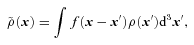
In Fig. 1, we plot the λ-space projections for point distributions drawn from a two-dimensional (left-hand side), one-dimensional (centre) and three-dimensional Gaussian function (right-hand side). These are models of a filament, wall and clump, respectively, and are each placed in a 200 h⁻¹ Mpc box. Smoothing will be done on a scale larger than the width of the structure, so the mock structures approximate a line, a plane and a point. We confirmed that the fingerprints are coordinate-independent by rotating the mock structures to random orientations.

Figure 1

Open in new tabDownload slide

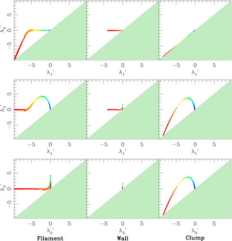
The structural ‘fingerprints’ for, from right-to-left, an isolated filament, a wall and a cluster in an otherwise uniform background, displayed in three projections of λ-space. The points are colour-coded by local density (blue, green, yellow, orange and red in order of increasing density) and inaccessible regions are shaded light grey, with eigenvalues defined such that λ′₁ < λ′₂ < λ′₃. All structures are smoothed on a scale much larger than their width.

Fig. 1 plots the distribution of the λ-parameters evaluated at the position of each galaxy, each interpolated on a 128 × 128 × 128 grid. The points in this figure are colour-coded by local density (blue, green, yellow, orange and red in order of increasing density). Note that the definition, λ′₁≤λ′₂≤λ′₃, entirely excludes four octants in λ-space, as well as portions of the remaining octants (delimited by the dashed lines in Fig. 1). In this and all subsequent multidimensional interpolations, we use a third-order polynomial routine given in Press, Flannery & Teukolsky (1986).

In all of the λ-space distributions, there is a tight grouping of blue points near the origin made up of background objects well away from the mock structures; the Hessian matrix of a uniform density field is all zeros. The remaining points trace the ‘fingerprint’ of the wall, filament or clump. Each fingerprint can be understood by considering the curvature properties of a Gaussian function. A Gaussian function has curvature given by

8

where f(x) is a one-dimensional Gaussian function with width, σ. At x= 0, the right-hand side of equation (8) is equal to −ρ(x)/σ². Moving to larger values of |x|, the value of this function increases, reaching a maximum at ⁠, and then switching sign at |x| =σ. Beyond this, the curvature of a Gaussian asymptotically approaches zero. The fingerprint of the wall follows naturally from this simple analysis. At all points near the wall centre (the densest regions, in red), the axis of structure will be either aligned with or orthogonal to the x coordinate axis – the density field has no y or z dependence so the curvature of the density field along those axes will always be zero. This means that will correspond to either λ′₁ (the smallest eigenvalue) or λ′₃ (the largest eigenvalue), depending upon the sign of the curvature along the x direction (which follows equation 8 after smoothing). Therefore, for |x| < σ

9

and for |x| > σ,

10

This explains the origin of the half-cross shape in the centre panel of Fig. 1.

For the clump, the direction of least curvature (and, therefore, the axis of structure) will be either parallel or perpendicular to the radial vector from the clump centre. Along this radial vector, the density field will follow the curvature properties of a Gaussian function, corresponding to λ′₃ in the bottom-right panel of Fig. 1. Orthogonal to this vector, the density field will always have negative curvature, meaning that the smallest two eigenvalues (λ′₁ and λ′₂; see the top-right panel) will always be negative and, by symmetry, equal in magnitude. All three eigenvalues increase with distance from the clump centre (in red) until the curvature of the Gaussian function maximizes at ⁠. Beyond this, λ′₃ drops and the fingerprint approaches the origin.

Finally, in the mock filament (left-hand column of Fig. 1), there is no z-dependence in the density field, so one of the λ-values will always be zero and the fingerprint will be restricted to one of the λ-space coordinate planes. Near the filament centre (in red), the curvature is negative orthogonal to the filament axis. This means that the two non-zero eigenvalues are negative and the fingerprint lies in the λ′₂–λ′₁ plane. Both of these eigenvalues will increase with distance from the filament centre, with the one corresponding to the radial eigenvector following the curvature of the one-dimensional Gaussian function (equation 8). At a cylindrical radius, ⁠, the curvature changes sign and this eigenvalue becomes positive (and, therefore, becomes λ′₃), after which the fingerprint remains on the λ′₃–λ′₁ plane and behaves like a projection of the clump fingerprint.

3.2 Wall and filament proportions

Neither the real data nor the cosmological simulations will have such a simple structure as the idealized models described the last section. To improve the realism of the tests, we will give the walls and filaments a finite extent, as well as place multiple structures within a single box.

The first set of tests (see Bond 2008) varied the length of the filament, ranging from six times to twice the smoothing length. As the filament size was reduced, the filament began to resemble a clump in λ-space. Filaments also have a wide range in width, as the very largest structures in the Universe (e.g. the Sloan Great Wall; Gott et al. 2005) have thicknesses of ∼ 50 h⁻¹ Mpc in redshift space, much greater than the widths of ‘typical’ filaments visible in redshift surveys. We generated sample filaments to test this width dependence, varying it between half and twice the smoothing length. We found that, even for very long filaments, the λ-space distributions show few of the characteristic ‘filament’ features unless the structure is narrower than the smoothing length. Thus, single-scale smoothing is insensitive to structures much wider than the smoothing length, suggesting that it will be useful to measure the scale-dependence of filamentarity with a series of measurements on different smoothing scales.

We have also considered the impact of nearby structures on the filament fingerprint. We find that fingerprint remains largely unchanged so long as the density of filaments is not so high that nearby structures are within one smoothing length of one another. In this limit, a smoothing length less than the average separation between structures is needed to distinguish them.

We conducted similar tests for walls, varying their side lengths, widths and number within a box. Points in the vicinity of a wall's edge will have λ-parameters similar to those of a filament and parameters for points near the corners will be like those of the clump. As with the filaments, a great deal of scatter was introduced when the structures were made very wide or very numerous.

Although the morphology of the λ-space distributions can vary with a structure's width, length or overdensity, there are discriminating features for each type of structure. Filaments can most easily be distinguished from clumps by a concentration around the λ′₃= 0 axis in the λ′₃–λ′₁ projection, while walls can be distinguished from filaments by a concentration on the λ′₂= 0 axis in the λ′₂–λ′₁ projection. In Section 7, these facts will be used to probe structure in cosmological simulations and SDSS galaxy data.

4 THE SIMULATION

Before we present the λ-space projections of the observed galaxy distribution, it is useful to explore the predictions of the standard cosmological model. A cosmological simulation allows us to develop our techniques on a data set not subjected to redshift distortions, sparse sampling and complicated window functions. Furthermore, we can simulate these effects in mock catalogues, providing a useful standard for comparison to the real SDSS data.

We use a series of cosmological cold dark matter (CDM) N-body simulations with Ω_m= 0.29, Ω_Λ= 0.71, σ₈= 0.85 and h=H₀/(100 km s⁻¹ Mpc ⁻¹) = 0.69 (Spergel et al. 2007). The simulation is performed within a 200 h⁻¹ Mpc box with 512³ particles, each with mass, m_p= 4.77 × 10⁹h⁻¹ M_⊙, and is run on a 92-node Beowulf cluster located at Princeton University. The positions and velocities of dark matter particles are output at six redshifts –z= 0, 0.3, 0.5, 1, 2 and 3. Because of memory restrictions, we split the simulation box into a 3 × 3 × 3 lattice in order to run a halo-finder and identify galaxies. Each subbox was padded with the particle data within 10 h⁻¹ Mpc of its boundaries. The padding size is an order of magnitude larger than the largest dark matter haloes, so edge effects are negligible.

We identified dark matter haloes with the HOP algorithm (Eisenstein & Hut 1998, hereafter EH98), which searches for peaks in the density field by moving from particle to particle until it reaches one that is in a denser environment than any of its neighbours. Densities are computed with an adaptive kernel with a length-scale set by the N_dens nearest particles, and the ‘hopping’ can occur to any of the N_hop nearest particles. Groups are then pruned, merged or disbanded depending on their peak and outer density thresholds (see EH98 for more details). Following EH98, we select N_hop= 16, N_dens= 64, N_merge= 4, δ_peak= 240, δ_saddle= 200 and δ_outer= 80. In addition, we keep only haloes with N≥ 8 particles. These parameters give halo distributions similar to those of a friends-of-friends algorithm (Huchra & Geller 1982) with a linking length of 0.2. We note that our results will be insensitive to the choice of the minimum halo mass as the faintest galaxies we will be studying (see Section 6.1) have a mean halo mass of ∼ 10¹² M_⊙, corresponding to N≃ 200 particles.

5 GAUSSIAN RANDOM FIELDS

In both the cosmological simulations and observed galaxy distribution, we wish to identify the morphological features that are unique to non-linear structure evolution; that is, features which are unlikely to appear in a Gaussian random field. If we wish to reveal these features in λ-space, then we should compare the Hessian parameters in observed or simulated data to those in a Gaussian random field with the same power spectrum. For the non-linear power spectrum, we use the prescription of Smith et al. (2003), with the concordance model parameters of Spergel et al. (2007).

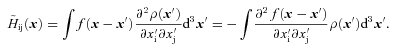
The left-hand column of Fig. 2 shows a slice from the z= 99 initial conditions for the dark matter distribution in a cosmological simulation, smoothed on a 5 h⁻¹ Mpc scale. In the top panel we plot the smoothed density field, while the smoothed λ′₁ and λ′₂-maps are given in the centre and bottom panels, respectively. The grey-scale map of λ′₁ gives a strong impression of filamentary structure. Note, however, that the λ-parameters are essentially edge-finders and both overdensities (whose edges are apparent in the λ′₁ map) and underdensities (λ′₂ map) will have boundaries. In a Gaussian random field, the overdensities and underdensities are statistically identical, so the maps are morphologically similar.

Figure 2

Open in new tabDownload slide

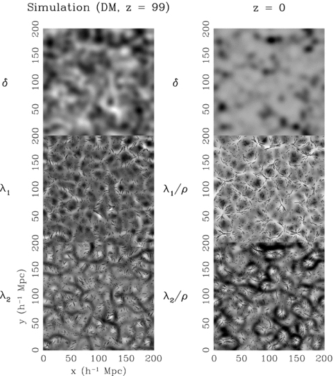
A slice (10 h⁻¹ Mpc deep) from the dark matter initial conditions of a cosmological simulation at z= 99 (left-hand column) compared with the same slice at z= 0 (right-hand column). The top row shows the density fields smoothed on a 5 h⁻¹ Mpc scale, while the middle and bottom rows show the corresponding λ′₁ and λ′₂-maps, respectively. The λ-maps have been normalized to the local density for the z= 0 dark matter distribution in order to emphasize the large-scale distribution of structures and provide an easy comparison to the initial conditions in the left-hand column. Bars have been plotted over the λ-maps to indicate the direction of the axis of structure at random points on the plane. The bar's length is proportional to the magnitude of λ′₁ at that point. It is clear to the eye that the axis of structure aligns with the local filamentary structure in the dark matter distributions. This alignment is absent in the initial conditions, despite a similar λ′₁ distribution.

On the right-hand side of Fig. 2, we show the same grey-scale maps for the z= 0 dark matter distribution in a cosmological simulation (see Section 4), but with the λ-parameters (centre and bottom panels) normalized to local density.2 Non-linear growth of structure amplifies overdense edges, and the low-contrast structures tend to become washed out in the raw λ-maps. After density normalization, however, the edges show a similar morphology to those in the λ′₁ and λ′₂-maps of the Gaussian random field, suggesting that the outline of the network of filaments and walls is already in place in the initial conditions (as was first suggested by Bond et al. 1996). Also included in the bottom two rows of Fig. 2 are bars indicating the direction of the local axis of structure. In the simulations, the axis of structure is nearly perfectly aligned with the λ′₁ edges in even the weakest strands, while in the Gaussian random fields, there is no obvious correlation between the axis of structure and the orientation of the edges. The direction of the axis of structure does not appear to be correlated on much more than a smoothing length in the Gaussian random field, while the simulations have structures that are aligned across the entire 200 h⁻¹ Mpc box!

6 GEOMETRY OF DARK MATTER AND MOCK GALAXY DISTRIBUTIONS

The two-point correlation function and power spectrum already provide a direct measure of the two-point properties of the large-scale distribution of matter, so we wish to extract from λ-space only that information which cannot be obtained from two-point statistics. In the left-hand column of Fig. 3, we show the λ-space distribution (smoothed on a 10 h⁻¹ Mpc scale) of a three-dimensional Gaussian random field. The contours illustrate λ-space distributions for points in the bottom 50 per cent of the real-space density distribution (black), between 50 and 75 per cent (blue) and the upper 25 per cent (red). The Gaussian random field was sampled in a (200 Mpc)³ three-dimensional grid in proportion to the local overdensity, which was normalized to match the amplitude of the ΛCDM non-linear power spectrum at each smoothing scale. No points were placed in grid cells having δ≤− 1 (< 0.1 per cent of the volume in all cases presented here). Within a given panel of Fig. 3, there is little variation in the size or shape of the contours as a function of overdensity, indicating no density dependence of structural morphology. The plot is generated from only one realization of a Gaussian random field, but finite volume effects are small at this smoothing scale.

Figure 3

Open in new tabDownload slide

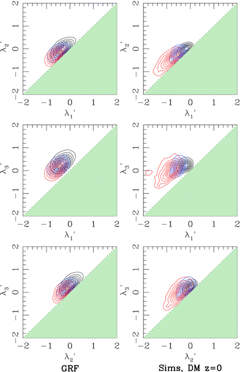
The λ-space projections for a three-dimensional Gaussian random field (left-hand column) and the simulated z= 0 dark matter distribution (centre). Contours represent the distribution of λ at the positions of dark matter particles (not grid cells) from a sampling of the fields. In the left two columns, contours are for different density subsamples, where black contours indicate the distribution of points in underdense regions (first or second quartile), blue contours in regions of intermediate density (third quartile) and red contours in the most dense regions (upper quartile).

In the large-scale distribution of matter, structure grows due to the gravitational effects of the total matter distribution. As such, we compute λ-space distributions at the positions of dark matter particles (not grid cells) in the z= 0, dark matter only simulation described in Section 4; these are shown in the right-hand column of Fig. 3. At high densities (red), the dark matter contours are extended because of the presence of overdense clumps. The low-density contours, however, are contracted relative to those of the Gaussian random field. The largest underdensities in the Gaussian random field have a positive curvature (and, therefore, positive λ-values) comparable to the negative curvature of the overdensities, while dark matter underdensities are voids with a very small spread in density and curvature. If non-linear growth of structure leads to the formation of filaments and/or walls in the dark matter distribution, there should be an excess in the regions of λ-space occupied by these fingerprints.

In order to bring out these regions, Fig. 4 shows the λ-space distributions of dark matter after subtracting a Gaussian random field with the same power spectrum (i.e. the difference between the columns in Fig. 3). Here, grey-scale density maps replace contours and there is no colour-coding for real-space density, but only points with density greater than the mean are included. A comparison of these plots with the fingerprints in Fig. 1 will help us determine which structures dominate the dark matter distribution at each smoothing scale. Note that the axes of each plot have been scaled in proportion to the amplitude of the dimensionless power spectrum at the appropriate smoothing scale, allowing for a direct comparison of structural morphology between scales.

Figure 4

Open in new tabDownload slide

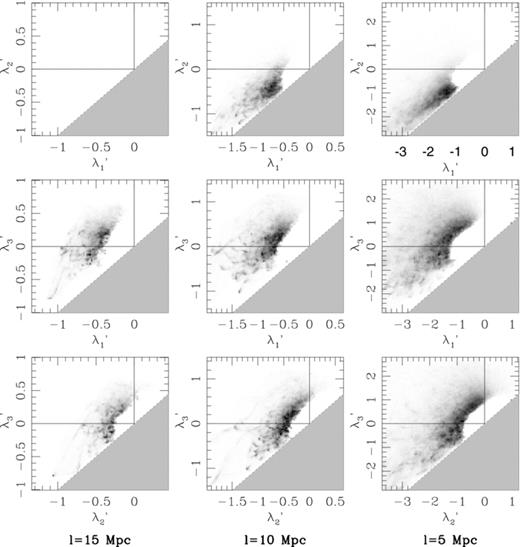
The λ-space projections for the z= 0 dark matter distribution, after subtraction by the λ-space distribution of a Gaussian random field with the same power spectrum. Grey-scale cells indicate those regions in which the dark matter distribution shows an excess over the Gaussian random field and for which the local density is greater than the mean, with darker cells indicating more of an excess. Regions showing no excess or regions showing a deficit are left blank. The axes of each plot have been scaled in proportion to the amplitude of the dimensionless power spectrum at the appropriate smoothing scale.

In order to make this comparison more quantitative, we will define a set of structural parameters,

11

where the mean is computed over the region of λ-space having λ_i < 0 and λ_j < 0. For example, R^λ₁₂ quantifies the mean axis ratio for structures that are negatively curved along at least two principal axes of the Hessian ellipse, allowing one to distinguish walls from filaments. A small value of R^λ₁₂ indicates that the axes have similar curvature and are more like filaments, while R^λ₁₂∼ 1 indicates the dominance of wall-like structures. Similarly, R^λ₂₃ can be used to distinguish filaments from clumps in regions with negative curvature along all three principal axes.

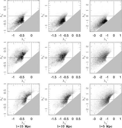
As shown in the right-hand column of Fig. 1, the densest parts of clumps lie on the lower boundary of λ-space (dashed line) in all three projections. Filaments concentrate on the lower boundary of the λ′₂–λ′₁ projection, as do clumps, but filaments also concentrate along the x-axis of the other two projections. In Fig. 4, we see that at both 15 and 10 h⁻¹ Mpc scales, the points in Fig. 4 appear to be shifted up towards the x-axis relative to the clump fingerprint. The distribution of points in the λ′₃ versus λ′₁ projection is broad and extends to very negative values of λ′₁, consistent with the presence of filaments in addition to clumps. At z= 0, it appears that filaments are the dominant over clumps at 15 h⁻¹ Mpc scales (R^λ₂₃= 0.605) and 10 h⁻¹ Mpc scales (R^λ₂₃= 0.602), with clumps becoming more prominent at 5 h⁻¹ Mpc smoothing scales (R^λ₂₃= 0.554). This evolution is most apparent in the highest contrast structures (small λ₂).

There is little evidence for walls at z= 0 at the smoothing scales shown. Walls manifest themselves as an excess of points near both λ′₂= 0 and λ′₃= 0. Although they are difficult to distinguish from filaments in the λ′₃ versus λ′₁ projection, there would be a clear overdensity of points along the x-axis of the top plots of Fig. 3 and near the origin of the bottom plots if walls were dominant features. The mean eigenvalue ratios suggest that structures become less wall-like at 5 h⁻¹ Mpc smoothing scales, with R^λ₁₂= 0.370, as compared to R^λ₁₂= 0.485 at 15 h⁻¹ Mpc smoothing scales.

In Figs 5 and 6, we present the λ-space distribution of structures at z= 1 and z= 3, respectively, smoothing on the same three comoving length-scales as in Fig. 4 (z= 0). The morphology of overdense structures in the dark matter distribution changes significantly at these redshifts. In all three λ-space projections, the distribution is concentrated closer to the x-axis at higher redshift, meaning that the larger eigenvalues decrease more rapidly than the smaller ones and overdensities are approaching spherical symmetry.

Figure 5

Open in new tabDownload slide

The same as Fig. 4, but for the z= 1 dark matter distribution.

Figure 6

Open in new tabDownload slide

The same as Fig. 4, but for the z= 3 dark matter distribution. At 15 and 10 h⁻¹ Mpc scales, distributions appear more wall like than those at z= 0, suggested by a shift towards the λ₂= 0 axis in the λ₂–λ₁ projection. Meanwhile, the λ-space distribution at 5 h⁻¹ Mpc scales is more filamentary, as suggested by a similar shift towards the λ₃= 0 axis in the bottom two projections. These latter projections are very similar to those for 15 h⁻¹ Mpc scales at z= 0.

At l= 15 h⁻¹ Mpc, all of the plots are more sparsely populated at high redshift, indicating that the λ-space distribution is closer to that of a Gaussian random field. This is especially true of λ′₃ versus λ′₂, which also shows no dramatic change in shape out to z= 1. In the λ′₃ versus λ′₁, l= 15 h⁻¹ Mpc projection, the most densely populated regions retain their shape and relative contrast out to the highest redshift (R^λ₁₃= 0.794 at z= 3 as compared to R^λ₁₃= 0.764 at z= 0), but some of the sparse features in the bottom-left corner fade by z∼ 1. Finally, the upper-left panel, λ′₂ versus λ′₁, undergoes strong evolution, with the tails at very negative eigenvalues disappearing and the bulk of the distribution moving to the λ′₂= 0 axis. This evolution is also demonstrated in R^λ₁₂, which drops from 0.599 at z= 3 to 0.485 at z= 0.

In Fig. 1, we see that walls are most easily distinguishable from other structures in λ′₂ versus λ′₁, with points concentrated along λ′₂= 0. Taken together, these facts are suggestive of wall-to-filament evolution at a l= 15 h⁻¹ Mpc comoving smoothing scale. The rapid fading of the λ′₃ versus λ′₂ map is also explained, as walls are concentrated towards the origin in these two eigenvalues and would be indistinguishable from a Gaussian random field. The signature of walls at high redshift are apparent in these plots, but they are of low contrast compared to the structures seen at smaller scales and lower redshift.

The two smaller smoothing lengths, l= 10 h⁻¹ Mpc and l= 5 h⁻¹ Mpc, exhibit a filament-to-clump evolution. In λ′₃ versus λ′₂, the distributions at both length-scales exhibit a tail along the dashed boundary that grows towards z= 0. This tail is populated by the points near the dense centres of clumps. A similar tail exists in λ′₃ versus λ′₁, but here the growth of individual filamentary features is also evident, with a concentration near the λ′₃= 0 axis. The eigenvalue ratios, R^λ₂₃= 0.647 at z= 3 and R^λ₂₃= 0.554 at z= 0, suggest filament dominance at l= 5 h⁻¹ Mpc across the entire redshift range, but with an evolution towards more ‘clump-like’ filaments.

It is interesting to compare the z= 1 projections for l= 10 h⁻¹ Mpc to the z= 0, l= 15 h⁻¹ Mpc projections. Their similarity suggests that the two length-scales are in similar stages of non-linear evolution, but at different times. This conclusion is supported by the eigenvalue ratios, with l= 15 h⁻¹ Mpc having R^λ₁₂= 0.485 at z= 0 and l= 10 h⁻¹ Mpc having R^λ₁₂= 0.497 at z= 1. That the smaller length-scales develop filamentary structure earlier is an indication of bottom-up structure formation; however, at a given comoving scale, structure evolves from walls to filaments to clumps, consistent with the ellipsoidal collapse picture of Zel'dovich (1970).

6.1 Mock catalogues in λ-space

In the SDSS data, we will be working with the observed galaxy distribution, so it is useful to generate λ-space projections for mock galaxies, generated by the methods described in Section 4. There are many fewer galaxies than dark matter particles in the box volume, so the signal will be much weaker and shot noise may be non-negligible at l= 5–10 h⁻¹ Mpc scales. More importantly, there may be interesting differences between the large-scale structures appearing in the dark matter and galaxy distributions. In order to populate the dark matter haloes with galaxies, we must know the relevant halo occupation distribution (HOD; Berlind & Weinberg 2002); the probability, P(N|M), that a halo of mass M will contain N galaxies.

Here, we use the parametrization of Zheng, Coil & Zehavi (2007), in which the probability of a halo of mass M containing a central galaxy is given by

12

Each central galaxy may be surrounded by one or more satellite galaxies, the mean number of which is given by

13

The number of satellite galaxies in a given halo is drawn from a Poisson distribution and has no upper limit. The free parameters, M_min, σ_{log M}, M₀, M₁ and α, have been derived from fits to SDSS galaxy catalogues. Table 1 of Zheng et al. (2007) provides the best-fitting HOD parameters for a series of absolute r-band magnitude cut-offs.

Once drawn from the relevant distributions, central galaxies are given the mean position and peculiar velocity of their associated dark matter halo, while satellite galaxies are each given the position and velocity of a randomly selected dark matter particle within the halo. When working with the SDSS data, we will construct a series of volume-limited samples, so the mock catalogues must be prepared to mimic the associated selection function.

One important difference between the redshift-space galaxy distribution and the dark matter distribution is the presence of fingers-of-god. These features, created by the peculiar velocities of galaxies in clusters, appear as very narrow filaments along the line of sight with widths ∼ 1 h⁻¹ Mpc and lengths up to ∼ 10 h⁻¹ Mpc. The mock catalogues must contain a model of these redshift distortions if they are to properly mimic the SDSS data. The ‘distorted’ positions of galaxies are computed as

14

where r is the position in real space, v is the galaxy's peculiar velocity and is the unit radial vector between the observer and the galaxy.

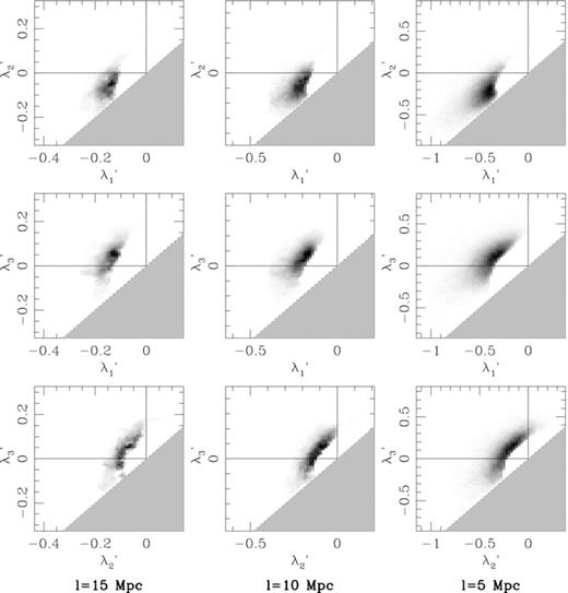
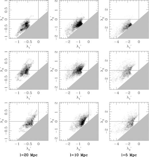
In Fig. 7, we plot the λ-space projections of an M_r < −20.5 mock galaxy sample projected into redshift space. The redshift distortions are applied from a vantage point with coordinates {-300,0,100} h⁻¹ Mpc relative to the origin of the box, selected to closely resemble the data samples constructed in the next section. The morphological characteristics of the λ-space distributions for l= 15 and 10 h⁻¹ Mpc are very similar to those of Fig. 4, though several features are different (e.g. the smearing of the previously noted clump signature in the bottom-left corner of λ′₃ versus λ′₁). The changes are most noticeable at l= 5 h⁻¹ Mpc, where all of the R^λ increase by ∼ 0.05 in the mock catalogues and the high-contrast features all but disappear. These high-contrast features are primarily due to clusters, which become lower-contrast fingers-of-god when projected into redshift space.

Figure 7

Open in new tabDownload slide

The λ-space projections for a z= 0 mock galaxy catalogue with M_r < −20.5, including redshift distortions.

With the construction of the mock catalogues and the development of the theoretical framework presented in Section 2, we now have all of the tools necessary to compare the real galaxy distribution to that predicted by the standard cosmological model. In the next section, we will present our galaxy sample, drawn from the SDSS, and use the λ-space distribution to make inferences about real large-scale structure.

7 FILAMENTS AND WALLS IN THE SDSS GALAXY DISTRIBUTION

The SDSS has imaged a quarter of the sky in five wavebands, ranging from 3000 to 10 000 Å, to a depth of r∼ 22.5 (Abazajian et al. 2009). As of Data Release 7, spectra have been taken of ∼ 930 000 galaxies, covering 8032 deg² and extending to Petrosian r∼ 17.7 (Strauss et al. 2002). Galaxy redshifts are typically accurate to ∼ 30 km s⁻¹, making the survey ideal for studies of large-scale structure. For this study, we need a portion of sky with relatively few coverage gaps to minimize the effect of the window function on the λ-space distributions. With this in mind, we construct three volume-limited subsamples from the northern portion (8 < α < 16 h and 25 < δ < 60) of the NYU Value-Added Galaxy Catalogue (NYU-VAGC; Blanton et al. 2005, through DR6), the first 80 × 80 × 220 (h⁻¹ Mpc)³ in size with M_r < −20 (Mr20), another 140 × 140 × 340 (h⁻¹ Mpc)³ in size with M_r < −20.5 (Mr205) and finally 170 × 170 × 400 (h⁻¹ Mpc)³ in size with M_r < −21 (Mr21). Absolute magnitudes were computed with kcorrect using SDSS Petrosian magnitudes shifted to z= 0.1 (and using h= 1). The sample properties of the galaxy distribution are given in Table 1 and the galaxy distributions are plotted in Fig. 8.

Figure 8

Open in new tabDownload slide

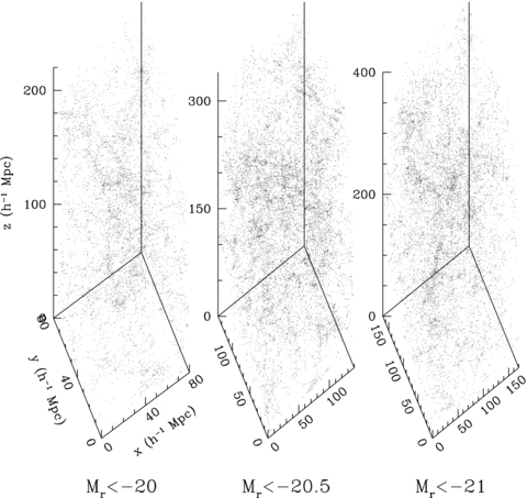
The three volume-limited samples taken from the SDSS VAGC large-scale structure sample with galaxies placed at their comoving positions based on the concordance cosmology. The location of the Milky Way is r= (250, − 20, 110) h⁻¹ Mpc, r= (310, − 20, 170) h⁻¹ Mpc and r= (400, − 25, 200) h⁻¹ Mpc in the Mr20, Mr205 and Mr21 samples, respectively, and the z-axes are parallel to the Galactic North pole.

All boxes are padded with 30 h⁻¹ Mpc of empty space and binned on a 128 × 128 × 256 grid, resulting in grid spacings of 1.09, 1.56 and 1.80 h⁻¹ Mpc in the Mr20, Mr205 and Mr21 subsamples, respectively. To correct for edge effects, we define a window function on the same grid such that

15

where S is the set of grid points within the SDSS survey volume and i is a grid cell within the subsample volume. The above window function was computed by smoothing the sample boxes on a 20 h⁻¹ Mpc scale and including in the window only those regions with densities more than 4 standard deviations below the mean density in the box. This is a crude approximation, but sample boxes were selected to lie in regions with few SDSS coverage gaps, so only a small fraction of grid cells are excluded (primarily near the box boundaries).

Once the window function and density fields have been computed on the grid, we smooth both with Gaussian kernels on the scales given in Table 1, giving and ⁠, respectively. The corrected density field is then

16

The first and second derivatives of the density field have zero mean on large scales (if the cosmological principle holds) and the kernels used to compute them will integrate to zero. As such, there is no need to renormalize the smoothed derivative fields near the padded regions. Rather, we need only subtract the signal from the edge artificially introduced by the padding. That is,

17

where is the matrix of smoothed second partial derivatives of the window function.

For each of the data samples listed in Table 1, we constructed a mock galaxy catalogue that matched the box dimensions, number density and padding of the SDSS data, incorporating redshift distortions according to the prescription described in Section 6.1. The processing on the mock galaxy catalogues and the real data were identical and they should be directly comparable, with the caveat that the mock catalogues were taken from a 200 × 200 × 200 (h⁻¹ Mpc)³ box periodic box, and therefore had to be repeated along the z-axis in order to match the dimensions of the data subsamples. As such, finite-volume uncertainties will be larger in the simulations.

In Fig. 9, we compare the two-dimensional λ′₁-maps between 10 h⁻¹ Mpc thick slices from the M_r < −20.5 subsample, its corresponding mock catalogue and the dark matter distribution. These data represent ∼ 3 per cent of the M_r < −20.5 subsample and the normalization and range of the grey-scales are identical between the two columns of each figure. The mean properties of each slice are superficially similar, although the slice from the mock catalogue has a large filament running through its centre, dominating the visual impression. In all maps, the axis of structure is oriented along edges in λ′₁, unlike the Gaussian random field shown in Fig. 2.

Figure 9

Open in new tabDownload slide

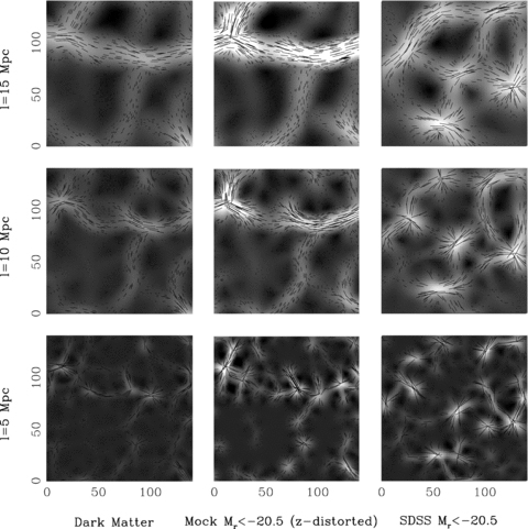
The two-dimensional λ′₁ distributions in slices from the z= 0 output of a ΛCDM cosmological simulation (dark matter and mock galaxy distributions, left-hand and centre columns), and the SDSS galaxy distribution (right-hand column), smoothed on a 15 h⁻¹ Mpc scale (top row), a 10 h⁻¹ Mpc scale (middle row) and a 5 h⁻¹ Mpc scale (bottom row). Bars have been plotted over the maps to indicate the direction of the axis of structure at each point in space. In all cases, the bar's length is proportional to the magnitude of λ′₁ at that point. The grey-scales are identical between the three columns. In all three samples and on all three smoothing scales, the axis of structure follows the minima in λ′₁.

The λ-space projections of the SDSS data are displayed in Fig. 10 for l= 20 h⁻¹ Mpc (Mr21), l= 10 h⁻¹ Mpc (Mr205) and l= 5 h⁻¹ Mpc (Mr21). For comparison, we present the corresponding λ-space distributions for the redshift-space mock catalogues in Fig. 11. At small scales, the value of λ′₁/λ′₂ at the positions of galaxies is generally near unity (diagonal lines) and the distribution morphologies are similar to those in the mock catalogues. Shot noise is more severe at these scales than at larger scales, so the similarity could be in part due to the extra power added by Poisson fluctuations. On 10 h⁻¹ Mpc scales, there are some indications that the real galaxy distribution may be more evolved than the simulated one, with all R^λ being smaller in the data by ∼ 0.05. The λ-space distributions for the data appear to have more high-contrast structures, including a tail of clump-like objects with near-unity values of λ′₂/λ′₃. If real, the discrepancy could suggest that the simulation is underestimating σ₈.

Figure 10

Open in new tabDownload slide

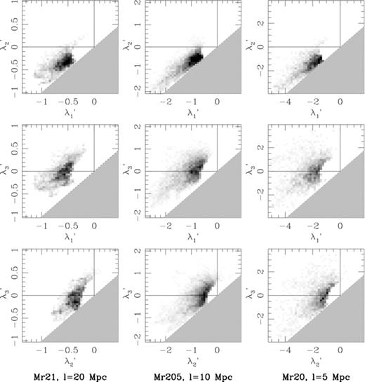
The λ-space projections for the three volume-limited subsamples of galaxies in the VAGC galaxy catalogue, smoothed on 20, 10 and 5 h⁻¹ Mpc scales. Grey-scale maps are the same as in Fig. 4.

Figure 11

Open in new tabDownload slide

The same as Fig. 10, but for the mock galaxy samples. Grey-scales and axis limits are the same between the two figures.

Finite-volume effects are apparent at the larger smoothing scales for all of the samples, where the R^λ-values are sometimes larger and sometimes smaller than their counterparts in the mock catalogues. At the largest smoothing scales, there is clear evidence for non-linearity and the λ′₂−λ′₁ projection shows evidence for both filaments and walls. Unlike the distributions at l= 5 h⁻¹ Mpc and l= 10 h⁻¹ Mpc, the data do not appear to be much more clump-like than the mock catalogues (R^λ₂₃= 0.61 in the data and R^λ₂₃= 0.54 in the mock catalogues). However, there is some suggestion that the data are less wall-like on the largest scales (R^λ₁₂ is smaller in the data by ∼ 0.08). This would also be consistent with a more evolved population, though finite-volume effects and uncertainties in the HOD make it difficult to say for sure.

8 DISCUSSION

8.1 A matter of scale

Mention of large-scale structure often brings to mind images of narrow, interconnected filaments with clusters at the interstices weaving their way between vast cosmic voids. Bond et al. (1996) dubbed this mental image the ‘cosmic web’, but we have avoided using that phrase in this paper. The components of a spider web are strands, which come together at nodes to make a variety of complex structures on larger scales. The same could be said for filaments in the dark matter distribution, but that is not a complete picture. We also know that these filaments are made up of bound dark matter haloes. These small-scale filaments can themselves be the building blocks for large-scale ones.

Some recent attempts to quantify and identify individual filamentary structures have not taken the multiscale nature of structure into account. For example, minimal spanning tree algorithms (e.g. Barrow, Bhavsar & Sonoda 1985; Colberg 2007) attempt to select filaments in the same manner as clusters, assuming that a step down up in linking length (i.e. down in density contrast) will allow the identification of the strands and full reconstruction of the web. Adaptive smoothing kernels and tessellation methods (e.g. Schaap & van de Weygaert 2000) enhance high-density regions in much the same way that simulations of galaxy formation adapt the mesh to treat star-forming regions, resulting in a nebulous combination of structure on small scales and large scales. There have also been attempts to use image segmentation (Aragón-Calvo et al. 2007) to select the most ‘prominent’ large-scale structures across a multitude of scales, and then remove them before looking for the next ones. Although this procedure makes sense on a given scale, removal of structures on one scale can cause one to miss structures on another.

We demonstrate the problem with this last approach using a 15 h⁻¹ Mpc deep slice from the SDSS Mr20 subsample (Fig. 12). At smoothing scales of both 10 h⁻¹ Mpc (upper-right panel) and 3 h⁻¹ Mpc (lower-right panel), the axis of structure appears to be aligned with the λ′₁ ridges, suggesting that matter is condensed into filaments/walls on both scales (see Fig. 2). Furthermore, the filaments/walls found on the smaller scale appear to be components of those on larger scales. If the structures found on the 10 h⁻¹ Mpc scale were removed before any of the smaller structures were identified, information would be lost. Conversely, if the smaller structures were all identified and removed first, there would be little left to find the larger ones.

Figure 12

Open in new tabDownload slide

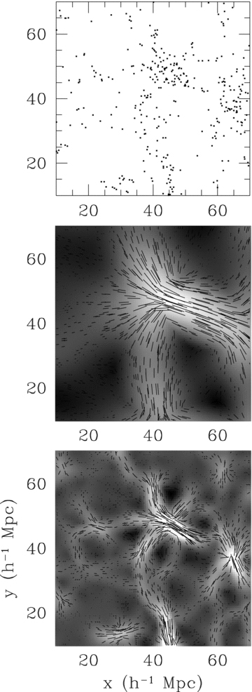
A two-dimensional demonstration of the structural hierarchy in a 15 h⁻¹ Mpc deep slice from the SDSS Mr20 subsample. Galaxies are plotted in the upper-left panel, and λ′₁ grey-scale maps are shown in the other two panels, smoothed on a 10 h⁻¹ Mpc scale (upper right) and a 3 h⁻¹ Mpc scale (lower right). Bars over the grey-scale maps indicate the local direction of the axis of structure and their length is proportional to λ′₁. Alignment of the axis of structure with the λ′₁ minima suggests that the structures are real on both scales (see Fig. 2). The filament- or wall-like structures seen on a 10 h⁻¹ Mpc scale are divided into smaller filaments or walls on the 3 h⁻¹ Mpc scale.

In this paper, we have presented results on a number of smoothing scales and demonstrated how structure changed across those scales. Filaments appear to be present on scales ranging from at least 5 to 25 h⁻¹ Mpc and are the dominant structures throughout most of that range. In Paper II, we extend these ideas by presenting a method to identify and characterize individual filaments.

8.2 Walls, walls, everywhere

There is evidence for a filament-to-clump progression as one smooths on progressively smaller scales in the z= 0 λ-space projections in both simulations and real data. Since smaller-scale overdensities collapse before larger ones, they should be in later stages of growth. The collapse of a large-scale overdensity might be expected to follow such a progression even if it were composed of smaller-scale condensed objects (such as dark matter haloes). The coherence of these large-scale filaments and walls would presumably depend upon the degree of fragmentation on intermediate scales.

One means of testing this picture is to look for walls in the very early stages of non-linear evolution. The z= 0 λ-space projections of the dark matter distribution show no convincing evidence for wall-like structures at scales as large as 15 h⁻¹ Mpc, but they may still exist on larger scales or earlier times. The former is difficult to explore in our 200 h⁻¹ Mpc simulation box, but we do have simulation outputs out to z= 3. In Fig. 13, λ′₁-maps for a 15 h⁻¹ Mpc smoothing length are plotted for a range of redshifts, along with bars indicating the axis of structure. Even at z= 3, it is clear that, unlike in a Gaussian random field, the axis of structure aligns with the λ′₁ edges (though it is impossible to distinguish filaments from walls in a two-dimensional projection). As discussed in Sections 6 and 8.1, there appears to be a progression in both time and smoothing scale of wall-to-filament-to-clump. If this progression holds at z= 0, we might expect to see wall-like structures dominating on ∼ 40–50 h⁻¹ Mpc scales.

Figure 13

Open in new tabDownload slide

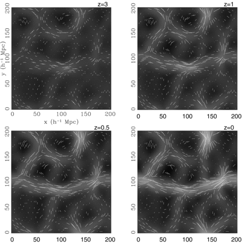
The λ′₁ grey-scale maps for a series of 10 h⁻¹ Mpc deep slices from the dark matter distribution, very similar to those in Fig. 2. The smoothing scale is 15 h⁻¹ Mpc and maps are plotted for z= 0, 0.5, 1 and 3. Bars indicate the direction of the axis of structure at random points on the grid, and the bar length is proportional to the local value of λ′₁. In all maps shown here, the grey-scale is scaled to the minimum and maximum of λ′₁ in the z= 0 map. The axis of structure aligns with minima in λ′₁ out to z= 3, unlike in Gaussian random fields.

The panels in the left-hand column of Fig. 14 show a subsample of dark matter particles in the 200 h⁻¹ Mpc simulation box satisfying λ′₁ < l_cutσ₁₅(z), where σ²₁₅ (z) is the variance of the density field at a given redshift when smoothed on a 15 h⁻¹ Mpc scale. Here, λ′₁ is measured with 15 h⁻¹ Mpc smoothing and l_cut is a dimensionless constant. The cut isolates very similar regions of space at each redshift, but the distribution of matter within those structures evolves a great deal with time. The regions isolated by the cut are very sheet-like, and at z= 3 the matter is smoothly distributed within the structures. As the evolution progresses, they collapse into filamentary and clump-like structures.

Figure 14

Open in new tabDownload slide

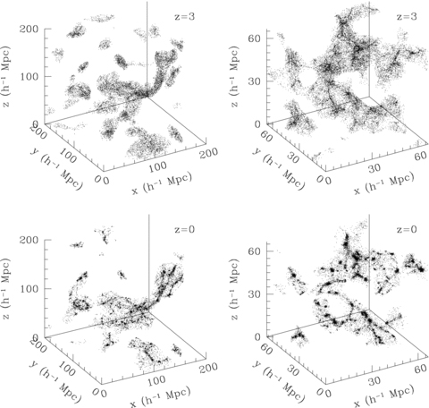
Selected dark matter particles in a 200 h⁻¹ Mpc simulation box at z= 0 and z= 3. In the left-hand column, particles are selected by the local value of λ′₁/σ₁₅(z) after 15 h⁻¹ Mpc Gaussian smoothing. This cut follows individual structures as they evolve. Most of the structures are sheets/walls at z= 3, but have collapsed into filaments by z= 0. In the right-hand column, 5 h⁻¹ Mpc smoothing is used in a 67 h⁻¹ Mpc box. On that scale, most of the structures are filamentary at z= 3, but have collapsed into clumps by z= 0.

Similarly, the right-hand column of Fig. 14 shows particles in regions of small λ′₁, but in a smaller box and on a smoothing scale of 5 h⁻¹ Mpc. Here, structures have begun to collapse into filaments at z= 3 and by z= 0 are primarily concentrated in clumps. Despite the evolution of the structures within the regions selected by a cut in λ′₁, the sizes and morphologies of the regions themselves change very little – they are still pancake-like at z= 0. This suggests that, even at low redshift, there should be evidence for wall-like structures in the galaxy and dark matter distributions on large scales, even if these walls are themselves made up of prominent filaments and clumps. As such, at all redshifts probed here, it can be the case that the majority of the mass in the Universe is in walls on large scales, which are made up of filaments on smaller scales, which are made up of clumps on still smaller scales.

9 CONCLUSIONS

With the eigenvalues and eigenvectors of the Hessian matrix, we can determine the type and orientation of structures in a continuous two- or three-dimensional density field. The ‘fingerprints’ of clumps, walls and filaments in a three-dimensional space of eigenvalues (λ-space) provide templates for comparison to the large-scale matter distribution. In addition, as a result of non-linear growth of structure, the third Hessian eigenvector (which is used to define the ‘axis of structure’) aligns with the axis of filaments in both two and three dimensions, retaining this alignment within approximately one smoothing length from the central axis.

We drew three volume-limited subsamples from the northern portion of the SDSS spectroscopic survey (using the NYU-VAGC catalogue) and computed their Hessian parameter distributions on a range of length-scales. These distributions were then directly compared to those found in a series of redshift-space mock galaxy catalogues generated from a cosmological simulation using the concordance cosmology. Results from this analysis include the following.

• The SDSS galaxy distribution is different from a Gaussian random field on all smoothing scales used here (up to 25 h⁻¹ Mpc), showing evidence for some combination of clusters, filaments and walls on all of these scales.

• Filaments are the dominant structures on smoothing scales of ∼ 10 h⁻¹ Mpc to ∼ 25 h⁻¹ Mpc, though there is some evidence for a transition to wall-dominance at ∼ 25 h⁻¹ Mpc. At 5 h⁻¹ Mpc clumps begin to dominate for the highest-contrast structures, but filaments are still apparent in the λ-space distributions.

• In very negatively curved regions of the galaxy density field (as would be found near walls, filaments and clusters), the direction of least curvature, indicated by the Hessian eigenvectors, points to other very negatively curved regions. In other words, the axis of structure aligns with minima in λ′₁. This occurs in projected slices at all smoothing scales studied here, providing a signature of non-linear growth even when non-linearities are not apparent to the eye in the density field.

• The λ-space projections of the SDSS galaxy distribution are very similar to those expected in a ΛCDM Universe with Gaussian random phase initial conditions. There is some evidence that the data are clumpier than the simulations.

• In projected slices, the λ′₁-maps of the galaxy distribution are morphologically very similar to those of a Gaussian random field. Since filaments and walls are oriented along minima in λ′₁, this suggests that the outline for the filament network can be determined from the initial conditions.

To complement the results presented above for the SDSS galaxy distribution, we generated λ-parameters at six redshifts in a ΛCDM cosmological N-body simulation, tracing the evolution of the matter distribution from z= 3 to z= 0. On comoving smoothing scales of 5 h⁻¹ Mpc, filament-dominance at z= 3 gives way to clump-dominance at z= 0. At z= 3 and on comoving scales of 15 h⁻¹ Mpc, the dark matter distribution is dominated by low-contrast walls, despite being only barely distinguishable from a Gaussian random field in λ-space. Structure on this smoothing scale becomes filament-dominated by z= 0. Finally, in projected slices, the axis of structure follows the minima in λ′₁ on smoothing scales as large as 15 h⁻¹ Mpc and epochs as early as z= 3. The same alignment is not seen in Gaussian random fields.

The λ-space distributions of the galaxy density field are only a first step towards a more complete description of large-scale structure. In Paper II, we describe a method for finding individual filamentary structures on a given scale, and then quantitatively evaluate the connection between filaments and galaxy clusters. Eventually, we hope to both extend our morphological studies to larger redshifts and characterize the galaxy populations in structures on a range of scales. We will compare the SDSS λ-space distributions to those found in hydrodynamic simulations, test the dependence of the λ-space distributions on the cosmological model and galaxy HOD, look for a dependence of galaxy properties on the local geometry (Park et al. 2007) and compare the galaxy λ-space distribution to that of the hot gas (e.g. Phillips 2003).

Funding for the SDSS and SDSS-II has been provided by the Alfred P. Sloan Foundation, the Participating Institutions, the National Science Foundation, the U.S. Department of Energy, the National Aeronautics and Space Administration, the Japanese Monbukagakusho, the Max Planck Society and the Higher Education Funding Council for England. The SDSS Web Site is http://www.sdss.org/.

The SDSS is managed by the Astrophysical Research Consortium for the Participating Institutions. The Participating Institutions are the American Museum of Natural History, Astrophysical Institute Potsdam, University of Basel, University of Cambridge, Case Western Reserve University, University of Chicago, Drexel University, Fermilab, the Institute for Advanced Study, the Japan Participation Group, Johns Hopkins University, the Joint Institute for Nuclear Astrophysics, the Kavli Institute for Particle Astrophysics and Cosmology, the Korean Scientist Group, the Chinese Academy of Sciences (LAMOST), Los Alamos National Laboratory, the Max-Planck-Institute for Astronomy (MPIA), the Max-Planck-Institute for Astrophysics (MPA), New Mexico State University, Ohio State University, University of Pittsburgh, University of Portsmouth, Princeton University, the United States Naval Observatory and the University of Washington.

We thank Jerry Ostriker for his many helpful comments and suggestions, Michael Blanton for his hard work and help with VAGC, and Jim Gunn, Neta Bahcall and J. Richard Gott III for serving on the committee to the thesis of which this work was a part.

REFERENCES