


Abstract
We examine the effects of gas expulsion on initially substructured distributions of stars. We perform N-body simulations of the evolution of these distributions in a static background potential to mimic the gas. We remove the static potential instantaneously to model gas expulsion. We find that the exact dynamical state of the cluster plays a very strong role in affecting a cluster's survival, especially at early times: they may be entirely destroyed or only weakly affected. We show that knowing both detailed dynamics and relative star–gas distributions can provide a good estimate of the post-gas expulsion state of the cluster, but even knowing these is not an absolute way of determining the survival or otherwise of the cluster.
INTRODUCTION
The vast majority of stars appears to form in environments with densities typically much greater than the field (Lada & Lada 2003; Bressert et al. 2010; King et al. 2012), but after a few Myr the majority of the stars are dispersed into the field (Lada & Lada 2003). The mechanism by which stars are dispersed is unclear, they may form unbound, or form in bound clusters which are then unbound by the expulsion of residual gas left-over after star formation (see below).
Star formation does not consume all of the gas in a molecular cloud, indeed it is estimated that at most 30 per cent of the gas is turned into stars (Dobbs et al. 2014; Padoan et al. 2014). Observations show that by 10 Myr, and probably well before, young stars are no longer associated with gas (Lada & Lada 2003). This gas has presumably been heated and expelled by feedback (ionization, mechanical winds and supernovae). It is interesting and important to examine how the stars respond to this gas loss and the corresponding (very significant?) change in the local potential.
Many authors have examined the effects of gas loss on stars (see Tutukov 1978; Hills 1980; Elmegreen 1983; Mathieu 1983; Lada, Margulis & Dearborn 1984; Elmegreen & Clemens 1985; Pinto 1987; Verschueren & David 1989; Goodwin 1997a,b, 2009; Geyer & Burkert 2001; Boily & Kroupa 2003a,b; Bastian & Goodwin 2006; Goodwin & Bastian 2006; Baumgardt & Kroupa 2007; Parmentier et al. 2008), but the majority of this work has concentrated on gas loss from clusters in which the stars and gas are both dynamically relaxed and in global virial equilibrium (but see Lada et al. 1984; Verschueren & David 1989; Goodwin 2009). If one assumes that the gas and stars in the cluster are well mixed and relaxed then the gas-to-star mass ratio is enough to derive the global star formation efficiency (SFE) in the cluster. However, Verschueren & David (1989) and Goodwin (2009) note that the exact dynamical state of clusters at the moment of gas expulsion is also extremely important and point-out that the SFE alone is not the most important factor in deciding the fate of a cluster.
Recently it has become very clear that not all stars form in relaxed, centrally concentrated clusters, and can often form in complex hierarchical/substructured distributions which follow the gas (Whitmore et al. 1999; Johnstone et al. 2000; Kirk, Johnstone & Tafalla 2007; Schmeja, Kumar & Ferreira 2008; Gutermuth et al. 2009; di Francesco et al. 2010; Könyves et al. 2010; Maury et al. 2011; Wright et al. 2014). It is still unclear which of clustered or ‘hierarchical’ is the main mode of star formation (or how and if they are connected), but it is clear that hierarchical is an important mode in many nearby low-mass star-forming regions.
In a hierarchical mode of star formation the stars and gas are not in anything close to equilibrium. Both will be in motion relative to one another as the stars respond only to gravity, where as the gas can suffer additional hydrodynamical effects and feedback. This means that the absolute and relative distributions of stars and gas at formation can change significantly before the gas is removed from the system. Therefore, the effect of gas removal on the stellar distribution depends not just on the relative masses of the stellar and gaseous components, but also on how they have dynamically evolved (see e.g. Kruijssen et al. 2012a).
This is the latest in a series of papers in which we have examined the response of complex, hierarchical systems to gas expulsion (see Smith et al. 2011, 2013a). The complexity of hierarchical distributions means that there is a very large parameter space to explore, and a wide variety of possible outcomes. In this paper, we expand on the work of Smith et al. (2011, 2013a).
SIMULATIONS
Since we wish to continue the work of Smith et al. (2011, 2013a), we use similar, simplified initial conditions for our simulations. We perform N-body simulations using the nbody6 code (Aarseth 2003).
As we describe in more detail below, equal-mass stars are distributed in a fractal distribution in a smooth and static background potential to mimic the potential of the gas in which they are embedded. Given that we use a static potential for the gas, we are unable to include active star formation in our models. However, we do not expect this to change the key conclusions of this study. The potential is then removed instantaneously to simulate gas expulsion.
This is clearly an extreme oversimplification in many ways. In reality, the gas is not distributed in a smooth spherical distribution, and both the gas and stars will move in response to changes in the global potential. The gas will also react to hydrodynamic forces and feedback (which is what eventually expel any remaining gas). Gas expulsion is unlikely to be instantaneous, rather gas will be lost at different rates in different regions, and dynamics can cause the stars and gas to decouple without any feedback.
We take this simplified approach rather than attempt to deal with the gas dynamics with a hydrodynamic method for two reasons. First, the practical issue of performing large ensembles of simulations – this is much quicker and easier with pure N-body simulations. Secondly, the complexity of the gas distribution would add large numbers of (largely unknown) parameters to our possible parameter space. We will return to discuss this issue later.
We choose equal-mass particles in order to avoid complex two-body interactions and mass segregation (see e.g. Allison et al. 2009 for the complications a realistic mass spectrum can add to an already complex problem). This will be addressed in more detail in a future paper (Blaña et al., in preparation).
Initial distributions
In all cases, we model the stellar distribution using N = 1000 particles with equal masses of 0.5 M⊙.
Using the box fractal method described by Goodwin & Whitworth (2004), we create 20 random realizations of fractal distributions, each with a fractal dimensions of D = 1.6, corresponding to a highly clumpy initial distribution within a radius of 1.5 pc. We use the same 20 stellar distributions for each background potential.
We start our simulations with two energies: initial virial ratios of Qi = 0.5 (warm), and Qi = 0 (cold). As we will show, even our Qi=0.5 simulations are not in equilibrium. Fractal clusters will then attempt to relax in pursuit of equilibrium and subsequently there are large variations in their virial ratio parameter. Thus, we measure Q instantaneously at two important epochs: the beginning of the simulation (Qi where ‘i’ donates ‘initial’), and the moment when gas expulsion begins (Qf where ‘f’ donates ‘final’). The cold systems start with the stars initially at rest relative to each other, this is unrealistic, but is the case where we expect the most rapid collapse and erasure of substructure.
The background potential and SFE
We work with three different static background potentials: (i) a Plummer sphere with Rpl = 1.0 pc and Mgas,tot = 3472 M⊙, (ii) a uniform sphere of gas with a maximum radius of R = 1.8 pc and Mgas, tot = 3455 M⊙ (equivalent to a Plummer sphere with Rpl = ∞), and finally (iii) a highly concentrated Plummer sphere with Rpl = 0.2 and Mgas,tot = 2053 M⊙. This choice of parameters ensures that we obtain a SFE = 0.2 for all three background potentials (i.e. we always have exactly 2500 M⊙ total mass within 1.5 pc, of which 2000 M⊙ is gas, and 500 M⊙ is stars).
In this work, we expel the gas instantaneously at early times in the evolution of the cluster i.e. within a few crossing times (1tcr ≈ 1.4 Myr), and compare to clusters with a later gas expulsion (∼7.5tcr).
Gas expulsion time
We simulate rapid gas expulsion by removing the background potential instantaneously. This is the most potentially destructive gas expulsion (see Baumgardt & Kroupa 2007).
As we wish to model the effects of early gas expulsion, we usually remove the gas potential instantaneously within two initial crossing times (1tcr ≈ 1.4 Myr). During this time, the initial distributions relax violently and tcr may no longer be a representative time-scale (see Section 2.5)
We first summarize the results from our previous studies before describing and explaining our new results.
Previous work
Numerical models of gas expulsion from initially virialized gas–star Plummer spheres have shown that a small fraction of stars can remain bound if the stars make up more than about 30 per cent of the initial system (in this case what is often assumed to be a direct measure of the SFE), and the majority of the stars will remain bound if the fraction is greater than 50 per cent (see e.g. Goodwin & Bastian 2006; Baumgardt & Kroupa 2007). The speed of gas expulsion is important with fast (instantaneous) gas expulsion being significantly more disruptive than slow (adiabatic) gas expulsion (see Lada et al. 1984; Baumgardt & Kroupa 2007).
Our initial conditions are a highly simplified, but hopefully realistic at a fundamental level, model of a fractal stellar distribution relaxing in a global gas potential before the removal of that gas potential. This is very different from the initially star–gas equilibrium distributions assumed in most previous studies.
Because the stellar distribution is highly out-of-equilibrium and also different from the gas potential, this means that the stellar distribution will violently relax. The initial fractal substructures will be erased and the stellar distribution will become smooth, whilst at the same time relaxing to fit the underlying static (gas) potential (see also Allison et al. 2009; Parker et al. 2014). This means that the stellar distribution will become more concentrated relative to the static gas potential as potential energy stored in substructure is distributed more smoothly (see e.g. Allison et al. 2009).
The LSF is analogous to the SFE quoted in many previous papers (although as noted by Verschueren & David (1989) and Goodwin (2009) this should really be called the effective SFE as its relationship to the true SFE is uncertain). Smith et al. (2011) show that the LSF will depend on the initial distribution of stars, the initial gas-to-star mass, and the initial energy of the stellar distribution (also see Kruijssen 2012b; Parmentier & Pfalzner 2013; Parmentier 2014).
Smith et al. (2011) find that there is a reasonably good relationship between the final bound fraction and the LSF at the point of gas expulsion for systems which have relaxed for more than two initial crossing times. However, Smith et al. (2013a) show that if gas expulsion occurs earlier, it is rather more complex than this suggests.
The longer the stars have to relax, the closer to a virialized, smooth distribution in equilibrium with the static gas potential they will become. Smith et al. (2013a) show two important consequences of this relaxation processes. First, the LSF changes with time and so the exact time of gas expulsion is very important. Secondly, the violent relaxation of the initially clumpy stellar distributions is stochastic and initial distributions that are initially ‘the same’ (i.e. drawn from the same generating functions) can evolve very differently, and at any particular point in time (i.e. at gas expulsion) can have quite different dynamics and be at different ‘stages’ in their relaxation. If gas expulsion occurs at early times (typically less than one crossing time, or around 1 Myr) then the LSF ceases to be a good predictor of the final bound fraction.
Smith et al. (2013a) attempted to quantify these effects and found that the virial ratio of the stars at the time of gas expulsion is also very important to the final bound fraction (as suggested by Goodwin 2009). In this study, we concentrate on examining the effects of the stellar virial ratio at the time of gas expulsion.
Motivation
In this paper, we extend the work of Smith et al. (2011, 2013a). We have two related questions that we wish to consider.
First, to what extent is it possible to predict the final bound fraction of the system? Secondly, is it ever practically possible (either observationally or theoretically) to predict the final bound fraction of a particular system?
In this paper, we concentrate mainly on the effects of the dynamical state of the stars at the time of gas expulsion (as measured by the stellar virial ratio).
We concentrate on systems which have not had many crossing times to relax. For the systems, we simulate here the instant of gas expulsion are typically 1–3 Myr, or less than two initial crossing times. This means that the initial substructured distributions have not had time to relax and are in the process of violent relaxation. It is worth noting that this corresponds to the age of the gas-free Orion nebula Cluster (Jeffries et al. 2011).
We will refer to the virial ratios of the systems, Q = T/|Ω| where T is the kinetic energy, and Ω the potential energy. Q = 0.5 corresponds to virial equilibrium, but we note that our systems (especially initially) are often not in any true equilibrium, even if Q = 0.5 (they might be formally virialized, but may not have equilibrium spacial or velocity distributions). Nevertheless as we shall describe below Q is a very useful measure.
The evolving dynamical state of the cluster
At the start of the simulation we have a very out-of-equilibrium distribution with a Qi = 0 or 0.5. The stars will immediately start to violently relax and erase the substructure present in the system (see also Allison et al. 2009; Parker et al. 2014). With our initial conditions there will always be an initial collapse of most of the stars. Violent relaxation rapidly, but very roughly, attempts to bring the system to a rough dynamical equilibrium (both virial equilibrium of the energies, and a smooth density field).
Therefore, the stellar component of the system rapidly changes its density distribution, size, and the way that energy is distributed. This means that any initial measures of size, energy etc. rapidly change, meaning that any useful time-scale such as crossing time also change.
We take as a measure of the state of the cluster the value of the virial ratio, Q, at any time as well as the rate at which the virial ratio is changing, |$\dot{Q}$|.
In Fig. 1, we show the evolution of the virial ratio with time for a typical system starting with Qi = 0.5. Even though this system starts in ‘virial equilibrium’ it immediately increases its Q, and then oscillates around Q = 0.5 with decreasing amplitude.
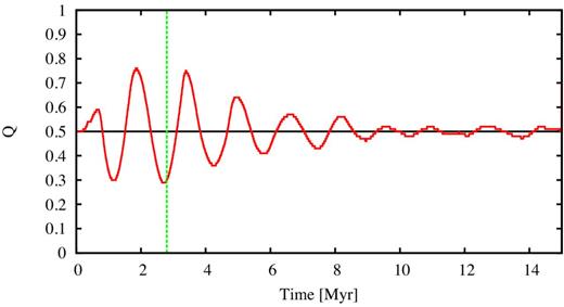
A representative example of the virial ratio variations with time of an out-of-equilibrium distribution of stars (a fractal in this case) inside a smooth background potential. As we study early gas expulsion, the smooth background potential is instantaneously removed before two crossing times occur (i.e. to the left of the vertical green dashed line).
What happens is that the cluster immediately starts to violently relax and attempts to collapse into the gas potential (thus Q rises as potential energy is converted into kinetic energy in the initial collapse). But the initial collapse is soon halted and the stellar distribution expands causing Q to fall, as the stars oscillate within the potential well of the cluster. Whilst this is happening substructure is also being disrupted, and within a few oscillations the system smooths out and the oscillations represent a ‘pulsation’ of a smooth cluster as it attempts to fully virialize. Therefore, the oscillations in Q with time provide an internal measure of the level to which the system has relaxed.
Gas expulsion times
When gas expulsion occurs is (yet another) key parameter in setting the final state of the system as quantified by the final bound fraction (see Goodwin 2009; Smith et al. 2011, 2013a). In our simulations this is modelled by the time at which we remove the static background gas potential to represent instantaneous gas expulsion. (Obviously this is a huge oversimplification which we return to in the discussion.)
In Smith et al. (2013a), we showed that the value of the virial ratio at the start of gas expulsion, Qf, is important – is the system in an expanding or contracting part of its relaxation process? However in Smith et al. (2013a), we chose a fixed instant in time for gas expulsion for all fractals. As each random realization of a fractal evolves differently, the exact virial ratio at the moment of gas expulsion was very varied, and uncontrolled.
In order to better control the dynamical state of the cluster at the point of gas expulsion, we artificially vary the instant at which gas expulsion occurs (between 0–2 crossing times) so as we can choose the virial ratio of the cluster. The upper limit for the time of gas expulsion is marked by the green dashed vertical line in Fig. 1. For example, in one series of ensembles we ensure that Qf = 0.5 by forcing gas expulsion to occur whenever the virial ratio happens to be at Q = 0.5.
Obviously real systems will not always expel gas at a pre-determined value of Qf = 0.5, so we also expel the gas at other times as Qf varies from subvirial (Qf ∼ 0.2) to supervirial (Qf ∼ 0.7).
The full set of initial conditions
To summarize our set of initial conditions:
We take ensembles of 10 or 20 statistically identical systems (all parameters from the same generating functions) with N = 1000 equal-mass stars with M = 0.5 M⊙ distributed as a D = 1.6 fractal with radius 1.5 pc. The velocities of the stars are scaled to give initial virial ratios for the stellar system in the background potential of Qi = 0 or Qi = 0.5.
These stellar distributions sit in a three different static background potentials. A Plummer sphere with Rpl = 1 pc, a highly concentrated Plummer sphere with Rpl = 0.2 pc, and a uniform sphere. All of them with a total mass of 2500 M⊙ within 1.5 pc that ensures an effective SFE = 0.2.
The systems are evolved and their time-evolving virial ratios are tracked. The instant of gas expulsion is varied in order to have gas expulsion occur when the final stellar virial ratio has a wide range of stellar virial ratios from subvirial (Qf ∼ 0.2) to supervirial (Qf ∼ 0.7). At the moment of gas expulsion the local star fraction (LSF) can be calculated.
They are then evolved until the simulation reaches 15 Myr (∼10.7 initial tcr) at which the number of stars still bound in a remaining cluster can be found to give the final bound fraction, fbound.
We reiterate that these are not very ‘realistic’ initial conditions, and there is much about them that is clearly artificial. However, even as artificially simplified as they are, they are still extremely messy and complicated. Their use is not to model reality directly, but rather to allow us to probe the physics behind relaxation and recovery after gas expulsion.
RESULTS
The key parameter that we wish to investigate is the fraction of stars that remain in a bound cluster after gas expulsion and the post-gas expulsion relaxation of the system. This ‘bound fraction’ (fbound) is the size of the naked cluster that remains. To measure the bound fraction we use the ‘snowballing method’. In this technique particles that are bound to the cluster are found in an iterative procedure, that corrects for the systemic velocity of the cluster at each iteration. (see section 2.6 of Smith et al. 2013b for a more complete description).
Final bound fractions
In Fig. 2(a), we show the final bound fraction, fbound, against the local star fraction, LSF, for all the simulations we have run in this paper.
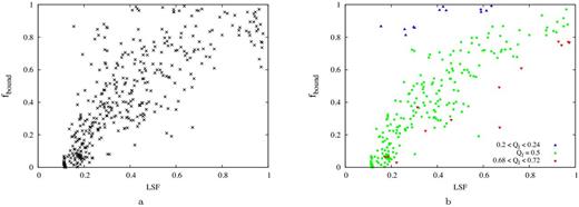
(a) Crosses show fbound against LSF at the time of gas expulsion for all the simulations carried out in this study (see text for details). (b) Simulations that are highly subvirial (Qf = 0.22–0.24; blue triangles), Qf = exactly 0.5 (green squares), or highly supervirial (Qf = 0.68–0.72; red inverted triangles) at the instant of gas expulsion
There is a vague trend that a high-LSF results in a high-fbound (i.e. the bottom right corner of Fig. 2 a is empty). But there is a huge amount of scatter in this figure, in particular around LSF of 0.2 can result in clusters with an fbound between zero and almost unity. For any particular value of LSF there is a scatter of at least 0.5 in fbound.
This might suggest that there is no way of estimating the final bound fractions of star clusters after gas expulsion. We show below that it is possible to understand the system and fairly accurately predict the final bound fractions if one knows both the LSF and stellar virial ratios at the time of gas expulsion.
Because of how we have (rather artificially) chosen our gas expulsion times we can split the simulations shown in Fig. 2(a) into groups depending on their final virial ratios. In Fig. 2(b), we only plot the simulations with 0.22 < Qf < 0.24 (blue), Qf ∼ 0.5 (green), and 0.68 < Qf < 0.72 (red).
It is clear from Fig. 2(b) that a significant amount of the scatter is due to the value of Qf at the time of gas expulsion. The 0.22 < Qf < 0.24 simulations all have fbound ∼ 1. The Qf ∼ 0.5 simulations show a rapid increase in fbound with LSF for low-LSF, then a very roughly linear increase. And the 0.68 < Qf < 0.72 simulations show a roughly linear increase in fbound with increasing LSF.
A simple physical model
In Fig. 3, we plot fbound against LSF for bins of different Qf increasing from low-Qf in the top left to high-Qf in the bottom right. Systems with initial virial ratios of Qi = 0.5 are marked by filled circles, those with Qi = 0 by open circles.
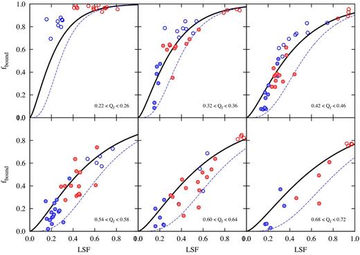
The fbound–LSF trend for different virial ratios. Colours represent the shape of the background gas, a Plummer sphere (blue) and a uniform sphere (red), filled circles are simulations with Qi = 0.5 and open circles are distributions with Qi = 0.0. The black solid lines and blue dashed lines are the fits from the model described in Section 3.2.
The black solid lines and blue dashed lines are a simple model fit to the data which we describe in this section. Note that the colours show the form of the gas potential which we will describe in the next subsection. For now we will concentrate on building a simple model to fit the fbound against LSF trends with different Qf.
We can construct a very simple analytical model that fits the results of our simulations surprisingly well (see Boily & Kroupa 2003a for a similar, but rather more detailed derivation).
As described above and in previous papers, the initial fractal stellar distribution will attempt to relax and virialize within the gas potential. What are important for the impact of gas expulsion are two quantities at the time of gas expulsion: the virial ratio Qf of the stars relative to the gas and the LSF. The LSF measures the relative masses of the gas and the stars within the stellar half-mass radius (see above). Therefore, the total mass (stars plus gas) Mtot in the region in which the stars are present is Mtot ∼ M*/LSF.
Let us denote quantities just before the gas expulsion with index 1 and just after the gas expulsion with 2.
In Fig. 3, we show fbound against LSF for various values of Qf. The solid black line is the fit from above which has no free parameters. This simple model describes the data points of our simulations very well, especially if we look at high-LSF and low-Qf values, i.e. when we do not lose many unbound stars (upper panels).
When we have high-Qf values as in the lower panels of Fig. 3 the simple model (solid black line) tends to overestimate the final bound fraction. We can apply a simple correction. Following the first estimate of fbound a fraction of stars is lost very rapidly after gas expulsion, and so the escape velocity falls by a further factor |$\sqrt{f_{\rm bound}}$| in equation (7). We then have to solve equations (7) and (8) iteratively which gives the blue dashed lines in Fig. 3. In most cases, the true values of fbound are enclosed between the solid black and blue dashed lines suggesting that reality is somewhere in between.
We have constructed a simple analytic approximation with no free parameters that estimates the final bound fraction from the values of the stellar virial ratio and LSF at the moment of gas expulsion. Given the simplifying assumptions we have made it is very gratifying that this seems to explain the results so well.
The effect of the gas potential
In Fig. 3, points are coloured according to the form of the gas potential: blue is a Plummer potential, and red a uniform sphere. There appears to be a very strong dependency on the form of the gas potential. In Fig. 3, systems with concentrated gas potentials (Rpl = 1 pc) shown by the blue markers are concentrated to the left of each panel with low-LSF and low-fbound. Systems with extended gas potentials (Rpl = ∞) shown by the red markers are towards the right with higher LSF and fbound.
Taken at face value this suggests that the form of the gas potential is crucial in determining the fate of a system. However, this is not the case. Rather it is due to a link between the form of the gas potential and the possible values of the LSF. The LSF measures the relative masses of gas and stars within the half-mass radius of the stars. Gas outside this radius is not taken into account. Even though the total mass in gas in the whole star-forming region stays constant, the LSF fluctuates as the half-mass radius of the stars fluctuates (this is the motivation for the introduction of the LSF by Smith et al. 2011).
Exactly how such a system will contract depends on the exact details of the initial fractal distribution, the initial virial ratio (Qi = 0 systems will contract more than Qi = 0.5 systems) and how relaxed the system has become. However, we find it does not depend on the shape of the background gas potential, as shown in Fig. 4. In the upper panel, symbols with error bars are the average LSF of simulations at the moment of gas expulsion. We include data points for (from left to right) Rpl = ∞ (uniform gas), Rpl = 1 pc and also Rpl = 0.2 pc (a very concentrated gas distribution). On the x-axis, we plot 1/Rpl in order to place all simulations on the same plot. There are two curves for the two different initial virial ratios (Qi = 0.0 and 0.5). There is a clear trend for the LSF to be lower as the gas becomes increasingly concentrated. To understand this, we must bear in mind that the LSF is a function of the total gas mass within the half-mass radius of the stars. Therefore, a change in LSF could arise from either a change in the amount of gas surrounding the stars, and/or a change in the half-mass radius of the stars as the gas scalelength is varied. We find that the half-mass radius is only a very weak function of the gas scalelength as shown in the lower panel of Fig. 4. Here, symbols with error bars are the average half-mass radius Rh of the stars. This weak dependency demonstrates that the strong dependency of the LSF on gas scalelength arises mainly for the following reason – by making the gas more concentrated, more gas is being placed about the stars, and the LSF is lowered.
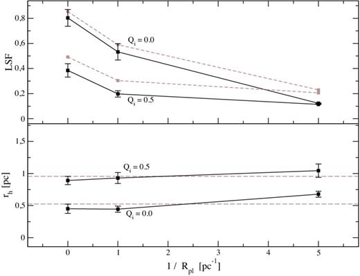
The variation of the LSF of the clusters due to the change in the concentration of the background gas. Top panel: the average of the LSF of the simulations against the inverse of their scalelengths. A black solid line connects simulations with the same initial virial ratio as labelled. Bottom panel: the half-mass radius is only weakly dependent on the gas scalelength. The average is shown by the horizontal dashed line. The brown dashed line in the upper panel is the recalculated LSF using a fixed half-mass radius with the average value.
To confirm that the small variation in Rh with gas scalelength does not play a strong role, we calculate the average Rh for each set (see horizontal dashed lines in the bottom panel of Fig. 4). Now we fix Rh to have the average value (i.e. a constant value for all gas scalelengths) and recalculate the LSF values at their new half-mass radius. The results are indicated by the brown dashed lines in the upper panel. The trend of LSF with gas scalelength is very similar, even when the stellar half-mass radius is fixed to be constant. This confirms that the strong dependency of the LSF on gas scalelength arises almost entirely for the following reason. Increasing the gas concentration places more gas about the stars, and does not change the stellar distribution significantly.
DISCUSSION AND CONCLUSIONS
Initially clumpy and irregular distributions of stars cannot be in dynamical equilibrium. As a result, they undergo violent relaxation with initially significant changes in their virial ratio as they expand and collapse, attempting to approach equilibrium. This occurs even when the clusters are initially ‘virialized’ (i.e. Qi = 0.5). These deviations are largest for very young star clusters, and decrease as the cluster settles down, as substructure is erased. As a result, the effects of gas expulsion at early times, before the system has relaxed, depend strongly on the instantaneous value of the virial ratio as well as the LSF (relative distribution of stars in the gas potential).
At later stages (>2 crossing times), it is known that the LSF becomes the key predictor of cluster survival from gas expulsion, with second-order modifications due to the cluster's dynamical state (Smith et al. 2013a). However, at these early stages when oscillations in the virial ratio are so large, we have shown that the dynamical state of the cluster may actually be equally influential (if not more influential) than the LSF.
A primary goal of studying the response of young, embedded star clusters to gas expulsion is to predict how well a cluster survives gas expulsion, based on its pre-gas expulsion properties. This study reveals that both the LSF, and the dynamical state can be important parameters dictating cluster survival to gas expulsion. Fortunately in our numerical studies, we can ascertain the exact value of the LSF and virial state. However, observationally, it may be incredibly challenging to measure either of these properties accurately. It is not inconceivable that the LSF might be calculated approximately by deprojection, although it would need to be a cluster caught very close to the instant of gas expulsion, or the LSF may later change. However, measuring the virial ratio of a real cluster is a huge challenge.
To worsen matters, our study reveals that in certain circumstances, even with a knowledge of both the LSF and virial ratio, the cluster survival maybe poorly constrained. For example, take a cluster with a low virial ratio (e.g. Qf = 0.34 at gas expulsion; upper-left panel of Fig. 3). If the cluster has an LSF∼0.2 (a reasonable physical value), the fbound–LSF trend rises very steeply. Such a cluster is equally likely to be near destroyed (have ∼90 per cent of its stars unbound), as only weakly affected (losing ∼30 per cent of its bound stars). Thus, it is possible that, even if the virial ratio were measured, the result could place the cluster in a region of parameter space where the cluster survival could be anything from weak mass-loss to near total destruction.
Comparing the panels of Fig. 3, we can see that clusters with LSF∼0.2–0.4 are the most sensitive to their dynamical state. In comparison clusters with high-LSF vary their resulting bound fractions very little, even for large changes in dynamical state. If LSF∼0.2 is a typical value, then these results suggest that clusters which are observed post-gas expulsion, must have been subvirial to avoid losing a large fraction of their stellar mass during the process.
Clearly our models are extremely simple conceptually. They lack a large number of physical processes that are also highly important in young star clusters. For example, our cluster stars have no initial mass function, we start our simulations with no binaries, we do not consider stellar evolution, and our treatment of the gas is highly simplified. Nevertheless, the use of such simple idealized models has enabled us to clearly determine the significant role of clumpy substructure and the dynamical state of the clusters on cluster survival following gas expulsion, through the use of controlled numerical experiments. This approach has revealed just how sensitive star clusters are to their dynamical state when gas expulsion occurs. We therefore suggest that real star clusters will be very sensitive, perhaps as sensitive as our model star clusters, to their dynamical state when the gas is expelled at early times.
Our key results may be summarized in the following.
For early gas expulsion (before 2 crossing times), we find the dynamical state of our model star clusters, measured at the time of gas expulsion, plays a key role in influencing cluster survival following gas expulsion. Star clusters may be highly super or subvirial in these early phases.
We show how the fbound–LSF trend can be well approximated with a very simple analytical model. The model matches the simulations best when the dynamical state is not extreme (i.e. highly super or subvirial).
Clusters which have LSFs in the range 0.2–0.4 (physically reasonable values) are most sensitive to the virial ratio at the instant of gas expulsion.
Clusters with low virial ratio have a very steep rise in the fbound–LSF trend. For such a cluster with an LSF∼0.2, it is therefore not possible to predict if the cluster will be heavily destroyed or only mildly affected – even knowing both the LSF and the virial ratio.
This study highlights the difficulties faced in trying to determine the survival rate(s) of real star clusters due to gas expulsion. At early times, the dynamical state of a cluster may be far from dynamical equilibrium, and this can significantly affect the clusters survival to gas expulsion. Thus, a best estimate of a cluster's survival is found measuring both the LSF and virial ratio. Accurately measuring these two parameters for a real cluster represents a huge observational challenge, in particular the dynamical state. Furthermore, some clusters may be situated in regions of parameter space where their survival to gas expulsion remains highly uncertain, even knowing both the LSF and virial ratio.
JPF acknowledges funding through FONDECYT regular 1130521 and a CONICYT Magister scholarship. RS was supported by the Brain Korea 21 Plus Program (21A20131500002) and the Doyak Grant (2014003730). RS also acknowledges support from the EC through an ERC grant StG-257720, and FONDECYT postdoctorado 3120135. MF is funded through FONDECYT regular 1130521. GNC acknowledges funding through FONDECYT postdoctorado 3130480. MB is funded through a CONICYT Magister scholarship, BASAL PFB-06/2007 CATA and DAAD PhD scholarship.
