


Abstract
We present deep 3-GHz Karl G. Jansky Very Large Array (VLA) observations of the potentially recoiling black hole CID-42 in the Cosmic Evolution Survey (COSMOS) field. This galaxy shows two optical nuclei in the Hubble Space Telescope/Advanced Camera for Surveys (HST/ACS) image and a large velocity offset of ≈1300 km s−1 between the broad and narrow Hβ emission line although the spectrum is not spacially resolved (Civano et al. 2010). The new 3 GHz VLA data have a bandwidth of 2 GHz and to correctly interpret the flux densities imaging was done with two different methods: multiscale multifrequency (MSMF) synthesis and spectral windows (SPWs) stacking. The final resolutions and sensitivities of these maps are 0.7 arcsec with rms = 4.6 μJy beam−1 and 0.9 arcsec with rms = 4.8 μJy beam−1, respectively. With a 7σ detection, we find that the entire observed 3-GHz radio emission can be associated with the south-eastern component of CID-42, coincident with the detected X-ray emission. We use our 3 GHz data combined with other radio data from the literature ranging from 320 MHz to 9 GHz, which include the VLA, Very Long Baseline Array (VLBA) and Giant Metrewave Radio Telescope (GMRT) data, to construct a radio synchrotron spectrum of CID-42. The radio spectrum suggests a type I unobscured radio-quiet flat-spectrum active galactic nucleus (AGN) in the south-eastern component which may be surrounded by a more extended region of old synchrotron electron population or shocks generated by the outflow from the supermassive black hole (SMBH). Our data are consistent with the recoiling black hole picture but cannot rule out the presence of an obscured and radio-quiet SMBH in the north-western component.
1 INTRODUCTION
During galaxy major mergers, the central supermassive black holes (SMBHs) that reside within the merging galaxies will form a bound binary SMBH system that can further merge (e.g. Volonteri, Haardt & Madau 2003; Hopkins et al. 2008; Colpi & Dotti 2009). At the time of the SMBH binary coalescence, strong gravitational wave (GW) radiation is emitted anisotropically, depending on the spin and mass-ratio of the two SMBHs, and to conserve linear momentum, the newly formed single SMBH recoils (Peres 1962; Bekenstein 1973). Recoiling SMBHs are the direct products of processes in the strong-field regime of gravity and they are one of the key observable signatures of an SMBH binary merger. As the SMBH recoils from the centre of the galaxy, the closest regions (disc and broad-line regions) are carried with it and the more distant regions are left behind depending on the recoil velocity (Merritt et al. 2006; Loeb 2007). Because GW recoil displaces (or ejects) SMBHs from the centres of galaxies, these events have the potential to influence the observed co-evolution of SMBHs with their host galaxies, as demonstrated by numerical simulations (Blecha et al. 2011; Guedes et al. 2011; Sijacki, Springel & Haehnelt 2011).
Only few serendipitous discoveries of recoiling candidates have been reported in the literature (Komossa, Zhou & Lu 2008; Shields et al. 2009; Batcheldor et al. 2010; Jonker et al. 2010; Robinson et al. 2010; Steinhardt et al. 2012; Bianchi et al. 2013; Koss et al. 2014) and systematic observational searches have resulted in no candidates so far (Bonning, Shields & Salviander 2007; Eracleous et al. 2012; Komossa 2012).
The Chandra-COSMOS source CXOC J100043.1+020637 (z = 0.359; Elvis et al. 2009; Civano et al. 2012b), also known as CID-42, is a candidate for being a GW recoiling SMBH with both imaging (in optical and X-ray) and spectroscopic recoil signatures (Civano et al. 2010, 2012a,b). CID-42 shows two components separated by ≈0.5 arcsec (≈2.5 kpc; see below for cosmology details1) in the Hubble Space Telescope Advanced Camera for Surveys (HST/ACS) image and embedded in the same galaxy. As presented in Civano et al. (2010, 2012a), the south-eastern (SE) optical source has a point-like morphology typical of a bright active galactic nucleus (AGN) and it is responsible for the entire (>97 per cent) X-ray emission of this system. The north-western (NW) optical source has a more extended profile in the optical band with a scalelength of ≈0.5 kpc, and the upper limit measured for its X-ray emission is consistent with being produced by star formation. In the optical spectra of CID-42 (VLT, Magellan, SDSS and DEIMOS; see Civano et al. 2012a,b), a velocity offset of ≈1300 km s−1 is measured between the broad and narrow components of the Hβ line (figs 5 and 6 of Civano et al. 2010).
Despite diverse scenarios being proposed to explain the nature of CID-42 (e.g. Comerford et al. 2009; Civano et al. 2010), the upper limit on the X-ray luminosity combined with the analysis of the multiwavelength spectral energy distribution favours the GW recoil scenario, although the presence of a very obscured SMBH in the NW component cannot be fully ruled out. The current data are consistent with a recoiling SMBH ejected approximately 1–6 Myr ago, as shown by detailed modelling presented in Blecha et al. (2013).
In this paper, we present new deep data at 3 GHz from the Karl G. Jansky Very Large Array (VLA) of the National Radio Astronomy Observatory (NRAO). For the analysis, we also make use of the radio data from the literature (Schinnerer et al. 2007; Smolčić et al. 2014; Wrobel, Comerford & Middelberg 2014; Karim et al., in preparation) to study the radio emission in CID-42 and bring further constraints on the nature of this source. Throughout the paper, a WMAP seven-year cosmology (Spergel et al. 2007; Larson et al. 2011) with H0 = 71 km s−1 Mpc−1, ΩM = 0.27 and |$\Omega _\Lambda$| = 0.73 is assumed.
2 VLA 3 GHZ DATA
2.1 Observations and reduction
We make use of the observations of the first 130 h of the Cosmic Evolution Survey (COSMOS; Scoville et al. 2007) field with the VLA in the S band (3 GHz, 10 cm; VLA-COSMOS 3 GHz Large Project; Smolčić et al., in preparation). The 2 GHz bandwidth is comprised of 16 × 128 MHz spectral windows (SPWs). We observed the 2 deg2 field with 110 h in A-configuration and 20 h in the C-configuration between 2012 and 2013. In order to cover the entire field, we required a total of 64 pointings. The quasar J1331+3030 was used for flux and bandpass calibration and J1024−0052 for gain and phase calibration. Weather conditions were excellent during the A-array observations while the C-array occasionally suffered from summer thunderstorms.
Calibration was done using the aipslite pipeline (e.g. Bourke, Mooley & Hallinan 2014) originally developed for the VLA Stripe 82 survey (Mooley et al. 2014, in preparation). The calibrated data were then exported to casa2 (version 4.2.1), where flagging (clipping in amplitude) was done separately for the A- and C-configuration data. All the epochs were concatenated into a single measurement set used for the imaging stage described below.
2.2 Imaging
To study the radio properties of CID-42 at 3 GHz, we imaged eight pointings (P19, P22, P30, P31, P36, P38, P39, P44) individually and joined them together in a mosaic (see Smolčić et al., in preparation for more details). CID-42 is located near the centre of pointing P36. Due to the wide bandwidth of the data, imaging can be done in various ways. One approach involves dividing the entire bandwidth into narrower SPWs which are then imaged separately and finally stacked together in the image plane (for details see Condon et al. 2012). This method gives accurate flux densities in each SPW because the flux density is approximately constant inside a sufficiently small bandwidth. Downsides include (i) loss of resolution as the lowest frequency SPW determines the resolution for the final stack, and (ii) uncleaned sources which do not have a sufficiently large signal-to-noise ratio (S/N) inside a single SPW. We describe the application of this method in Section 2.3.
Another imaging approach is the multiscale multifrequency (MSMF) method developed by Rau & Cornwell (2011) which allows the usage of the entire bandwidth at once to calculate the monochromatic flux density at a chosen frequency. It uses Taylor term expansion in frequencies along with multiple spatial scales to deconvolve the map and includes a map of spectral indices calculated from the Taylor series. Throughout the paper we define spectral index α as Fν ∝ να, where Fν is flux density at frequency ν. The final resolution is not limited to the lowest frequency beam size because all of the SPWs are used in the deconvolution. For more details on this algorithm, see Rau & Cornwell (2011) and Rau, Bhatnagar & Owen (2014). We describe this approach in Section 2.4. We applied both imaging methods using the casa task CLEAN.
2.3 SPWs stack
To correctly stack maps, it is necessary that they all have the same resolution which is defined by the lowest frequency SPW. We used the robust parameter in the Briggs weighting scheme to achieve similar resolutions in different SPWs. With higher robust value (towards natural weighting) it is generally expected to get lower rms noise and a larger synthesized beam, but worse sidelobes. However, sidelobe contamination started to drastically degrade the map quality after a certain robust value. The final robust values we converged on are listed in Table 1. They give the optimum tradeoff between resolution, rms and sidelobes. After each SPW is cleaned, it is convolved to a common resolution of 0.9 arcsec using the casa toolkit function convolve2d and then corrected for the primary beam (PB) response with the casa task impbcor.
Summary of robust parameters, flagged data and final rms values for each SPW. The rms noise is calculated after convolution to a common beam size but before PB correction. Last column shows which array data were entirely flagged due to radio frequency interference (RFI).
| SPW | ν (GHz) | Robust | rms (μJy beam−1) | Flagged |
|---|---|---|---|---|
| 0 | 2.05 | 0.0 | 25.6 | – |
| 1 | – | – | – | A+C |
| 2 | – | – | – | A+C |
| 3 | 2.44 | 0.0 | 20.2 | – |
| 4 | 2.56 | 0.5 | 16.5 | – |
| 5 | 2.69 | 0.5 | 17.4 | – |
| 6 | 2.82 | 0.5 | 17.1 | – |
| 7 | 2.95 | 0.5 | 16.0 | – |
| 8 | 3.05 | 0.5 | 16.0 | – |
| 9 | 3.18 | 0.5 | 14.4 | – |
| 10 | 3.31 | 1.0 | 13.0 | – |
| 11 | 3.44 | 1.0 | 12.8 | – |
| 12 | 3.56 | 1.0 | 12.8 | – |
| 13 | 3.69 | 1.5 | 19.5 | C |
| 14 | 3.82 | 1.5 | 30.9 | C |
| 15 | 3.95 | 1.5 | 32.0 | C |
To optimize the S/N in the final stack, the SPW maps have been stacked weighting each pixel by the inverse of its local noise squared. Thus, each pixel in the sum is assigned a weight of w = (A(ρ)/σ)2, where A(ρ) is the PB response, ρ is the distance from the pointing centre and σ is the rms. Note that the PB response entering this term only scales the rms (σ drawn from the cleaned map prior to PB correction) as a function of distance from the pointing centre. Because the FWHM of the PB (and therefore noise) changes between SPWs, not all frequencies will contribute the same amount to each pixel in the final stack. To account for this effect, a map of effective frequencies is also created by averaging the SPW frequencies using corresponding noise weights for each SPW with the casa task immath. In total, we produced three stacks (at a resolution of 0.9 arcsec): one for the full bandwidth using all of the SPWs (SPWs 0–15) reaching an rms of 4.8 μJy beam−1, one for the low-frequency sideband (SPWs 0–8) reaching an rms of 6.9 μJy beam−1, and one for the high-frequency sideband (SPWs 9–15) reaching an rms of 6.5 μJy beam−1. In Fig. 1, we show cutouts centred on CID-42 in each map we created. Resolution, rms and effective frequency of these maps are listed in Table 2.
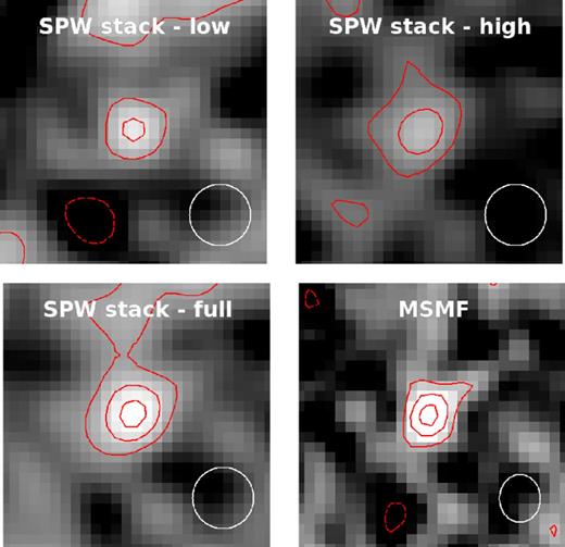
Cutouts of 4 arcsec on the side centred on CID-42: low-frequency SPW stack, high-frequency SPW stack, full SPW stack and MSMF map. All SPW stacks have the same resolution of 0.9 arcsec, while the MSMF map has a resolution of 0.7 arcsec. The synthesized beam size is shown in the lower-right corner of each panel. Contours of ±2σ, ±4σ and ±6σ are overplotted in red (negative contours are drawn with dashed lines). Local rms in each map is listed in Table 2.
Radio data used for the CID-42 flux density analysis along with the corresponding resolution and local rms noise inside the maps. CID-42 is resolved in the 1.4-GHz VLA map and marginally resolved in the 3 GHz MSMF map where integrated flux density is also reported in parentheses, for all other maps peak flux density is reported.
| ν (GHz) | Instrument | Resolution (arcsec) | rms (μJy beam−1) | Flux density (μJy beam−1) | Author |
|---|---|---|---|---|---|
| 0.32 | VLA | 6 | 442 | <1326 | Smolčić et al. (2014) |
| 0.325 | GMRT | 10.8 | 80 | 240 ± 80 | Karim et al. (in preparation) |
| 1.4 | VLA | 1.5 | 10 | 85 ± 10 | Schinnerer et al. (2007) |
| (138 ± 38 μJy) | |||||
| 1.5 | VLBA | 0.015 | 13 | <78 | Wrobel et al. (2014) |
| 2.7 | VLA (SPW stack – low) | 0.9 | 6.9 | 31.2 ± 6.9 | This paper |
| 3.4 | VLA (SPW stack – high) | 0.9 | 6.5 | 35.4 ± 6.5 | This paper |
| 3.1 | VLA (SPW stack – full) | 0.9 | 4.8 | 33.2 ± 4.8 | This paper |
| 3 | VLA (MSMF) | 0.7 | 4.6 | 32.5 ± 4.6 | This paper |
| (39.7 ± 9.5 μJy) | |||||
| 9 | VLA | 0.32 | 6 | <18 | Wrobel et al. (2014) |
2.4 Multiscale multifrequency
Imaging was independently performed with MSMF using the casa task clean that uses the entire 2 GHz bandwidth at once (Rau & Cornwell 2011). Each pointing was cleaned individually. Two Taylor terms were used in the frequency expansion (nterms=2) along with three resolution scales. The final synthesized beam size was 0.7 arcsec × 0.6 arcsec. We used Briggs weighting with a robust value of 0.5 to produce a map with low sidelobe contamination and good rms. After the deconvolution, wideband PB correction was applied using the casa task widebandpbcor. The resulting maps include flux densities at a reference frequency of 3 GHz along with the spectral index map (α map) all corrected for the PB response. The rms of the MSMF map is 4.6 μJy beam−1 and an MFMS map stamp centred at CID-42 is shown in Fig. 1.
2.5 CID-42: flux and size at 3 GHz
To properly extract the flux density of CID-42, information about its size is needed. A source is considered resolved if it is larger than the beam size; however, this is a function of S/N ratio as described in Bondi et al. (2003). Thus, to estimate whether CID-42 is resolved, we need to know how the integrated-to-peak flux density ratio Sint/Speak behaves as a function of S/N in our mosaic. For this purpose, we use the aips task SAD (search and destroy) to extract a catalogue of sources, their positions and flux densities over the mosaic. The catalogue extraction was performed in the same way as for the other VLA-COSMOS surveys, described in detail in Schinnerer et al. (2007, 2010) and Smolčić et al. (2014). We have compared the peak flux density with the integrated flux density of CID-42, as well as its peak-to-integrated flux ratio relative to those of other sources in the mosaic as a function of S/N. From this analysis, we conclude that CID-42 is unresolved at a resolution of 0.9 arcsec and that it is marginally resolved at 0.7 arcsec. We report the peak flux density of CID-42, drawn from the SPW stack map to be 33.2 ± 4.8 μJy and from the MSMF map 32.5 ± 4.6 μJy. Since CID-42 is only marginally resolved in the MSMF map, we report its integrated flux density of 39.7 ± 9.5 μJy, but we do not use this value in the spectral analysis. The error of peak flux density is determined from the local rms obtained via fitting the histogram of the pixel flux density values with a Gaussian, and the error for the integrated flux density is drawn from the elliptical Gaussian fit.
As the resolution of our 3 GHz data is around a factor of 2 higher than that of the large VLA-COSMOS 1.4 GHz data (Schinnerer et al. 2007), to test whether we may be out-resolving a fraction of the flux density at 3 GHz we used two methods to match the resolution of the 3 GHz map to the 1.4 GHz map. First, we convolved the 3 GHz map to a resolution of 1.5 arcsec, matching that of the 1.4 GHz map. Peak flux density of CID-42 in this map is 36.8 ± 7.3 μJy beam−1. Secondly, in the cleaning process, we weighted the visibilities with the Gaussian taper in the uv-plane. This approach gave a peak flux density of 34.6 ± 6.3 μJy beam−1. Both methods result in flux densities consistent with the higher resolution map within the error bars.
3 RADIO DATA ANALYSIS
3.1 Image analysis
Table 2 lists all the radio data used for the CID-42 analysis presented here, their resolutions and rms in the corresponding maps. In the top panel of Fig. 2, we show the HST/ACS image (Koekemoer et al. 2007) of CID-42 with contours from the 1.4-GHz (black) and 3-GHz (magenta and blue) radio data overlaid. The resolution of 1.5 arcsec at 1.4 GHz (Schinnerer et al. 2007) is not accurate enough to distinguish whether the radio emission is associated with the NW or the SE optical source (see also Civano et al. 2010). However, the 3 GHz data presented here at a resolution of 0.7 arcsec show that the 6σ contours are coincident with the SE component. The peak of the 3 GHz radio emission is located at |$\alpha _{2000.0}=10^{{\rm h}} 00^{{\rm m}} 43 {.\!\!^{{\mathrm{s}}}}148,\ \delta _{2000.0}= + 2 {^\circ }06 {^\prime }37 {^{\prime\prime}_{.}} 06$|. The offset between the centre of the SE component in the HST image and the centre of the VLA 3 GHz emission is 0.08 arcsec. This value is within the positional error of 0.1 arcsec estimated from the ratio of resolution and S/N which dominates the positional uncertainty of faint sources. We compared the positions of 30 sources measured with the Very Long Baseline Array (VLBA) by Herrera Ruiz et al. (in preparation) with our 3 GHz mosaic and found that positional errors in our mosaic are less than 0.03 arcsec. This constrains the positional error of bright sources (S/N between 40 and 900) inside our mosaic. The low S/N sources positional error is therefore dominated by the mentioned term.
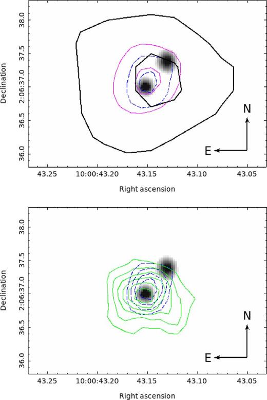
Top: HST/ACS grey-scale image showing the two optical components of CID-42 with contours from the radio data overlaid. For each radio map, two contour lines are shown that correspond to 3σ and 6σ. Thick black lines show data from the VLA 1.4-GHz large map from Schinnerer et al. (2007) with σ = 10 μJy beam−1. Thin magenta lines and dashed blue lines are from the VLA 3 GHz SPW stack map and MSMF map with the local rms of 4.8 and 4.6 μJy beam−1, respectively. Bottom: HST/ACS grey-scale image of CID-42 with contours from the adaptively smoothed X-ray Chandra High Resolution Camera image with a 3 pixel radius Gaussian kernel by Civano et al. (2012b) in green and VLA 3 GHz MSMF map with 1σ steps starting from the 3σ in blue.
In the bottom panel of Fig. 2, we show that radio emission at 3 GHz is coincident with the X-ray emission (Civano et al. 2012b). As described in detail in Section 2.5, CID-42 is unresolved at a resolution of 0.9 arcsec meaning that the FWHM 3 GHz radio emission is constrained to a region <4.5 kpc (at the source redshift) centred at the SE optical component. Since CID-42 is marginally resolved in the MSMF map at a resolution of 0.7 arcsec, we calculated its deconvolved size. The deconvolved FWHM major axis is 0.6 arcsec and minor axis 0.1 arcsec (corresponding to 3 and 0.5 kpc, respectively) with a position angle of −36° measured from north to east which could indicate an elongated shape of the source. However, better resolution and deeper data are needed to confirm this.
3.2 Spectral analysis
Fig. 3 shows spectral features of CID-42 across a frequency range of 320 MHz to 9 GHz. Schinnerer et al. (2007) observed CID-42 at 1.4 GHz and 1.5 arcsec resolution within the VLA-COSMOS survey. They find the source resolved at that resolution and report an integrated flux density of 138 ± 38 μJy. Wrobel et al. (2014) found no detection using a high resolution of 0.015 arcsec VLBA at 1.5 GHz and report a 6σ upper limit of 78 μJy beam−1. Wrobel et al. (2014) also did not detect the source at the higher frequency of 9 GHz using the VLA with a 3σ upper limit of 18 μJy beam−1. In Fig. 3, we further plot the 325-MHz flux density of 240 ± 80 μJy beam−1 from the Giant Metrewave Radio Telescope (GMRT) data (Karim et al., in preparation). The GMRT gives a tentative 3σ detection for CID-42, but since we know the source location and we expect that it is unresolved at a resolution of ≈10 arcsec this may justify a peak flux density measurement. For this reason, the spectrum shown in Fig. 3 is not strongly constrained by the 325 MHz measurement.
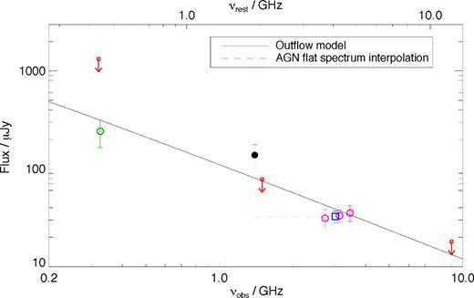
Radio spectrum of CID-42. Values are listed in Table 2. Black point marks the total integrated flux density from the 1.4-GHz VLA data (Schinnerer et al. 2007). Magenta points are peak flux densities from SPWs stacks from our new VLA 3 GHz data. Flux density from the MSMF cleaned map is shown with a blue square. Green point is peak flux density from the GMRT map (Karim et al., in preparation). Red arrows show upper 3σ limit from the 320 MHz VLA (Smolčić et al. 2014), 3σ limit from the 9-GHz VLA data, and 6σ limit from the 1.5-GHz VLBA data (Wrobel et al. 2014). The flat spectrum interpolation for AGN is plotted with red dashed line. Black line corresponds to a shock generated by outflow model (see the text for details).
In the 2 GHz bandwidth centred at 3 GHz, the galaxy shows slightly inverted spectra. This behaviour is evident in the flux densities extracted from the SPW stacks (see Fig. 3) and also from the spectral index calculated in the MSMF alpha map where α = 0.4 ± 0.3. For the sake of simplicity, we will treat this as a flat spectrum (α = 0). Using only the MSMF value, the flux density of CID-42 at 3 GHz corresponds to rest-frame spectral luminosity of L3GHz ≈ 1 × 10²² W Hz−1. Based on radio-loud versus radio-quiet definitions in the literature relying only on radio luminosity values (e.g. Miller, Peacock & Mead 1990, see also Baloković et al. 2012), this falls into the radio-quiet regime.
To test the consistency between the two different wideband imaging methods and the robustness of our 3 GHz data in general and thus that for CID-42, we have closely examined the spectral behaviour of 109 sources in the mosaic in different locations within the PB. In Fig. 4, we show eight representative sources over a broad S/N range (from 230 to 5). In the spectral plots, we also show our 3-GHz flux densities with the 1.4-GHz Large Project catalogue values (Schinnerer et al. 2007) and the 325-MHz GMRT data (Karim et al., in preparation). We find that both imaging methods (SPW stack and MSMF) give consistent flux densities, also consistent with the flux densities at lower frequencies. Thus, we conclude that our map is robust with no systematics for sources at either high or low S/N.
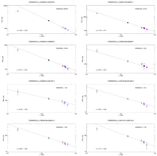
Flux densities for selected sources as a function of frequency inside the VLA-COSMOS pointing containing CID-42 at different S/N ratios. Filled symbols are used for integrated flux densities of resolved sources and empty symbols for peak flux densities of unresolved sources. Black points mark the flux density from the 1.4-GHz large project catalogue (Schinnerer et al. 2007). Magenta points are flux densities from the low-frequency, whole-bandwidth and high-frequency SPW stack from the VLA 3 GHz data. Green points are peak flux densities from the GMRT map (Karim et al., in preparation). Flux density from the MSMF cleaned map is shown with a blue square. Black dashed line corresponds to spectral index derived from the 1.4 and 3 GHz point. Error bars represent the local rms for peak flux densities and fit error for integrated flux densities.
4 DISCUSSION
The unresolved emission at 0.9 arcsec and flat spectrum we derived here for CID-42 at 3 GHz (see Fig. 3) suggest that the entire observed radio emission at 3 GHz (with 2 GHz bandwidth) may arise from an AGN within the SE component. The VLBA upper limit at 1.5 GHz by Wrobel et al. (2014) is consistent with the flat spectrum AGN picture, as the VLBA can observe scales up to 150 mas (750 pc) but it is not sensitive to star formation induced emission. The non-detection at 9 GHz (Wrobel et al. 2014) could be explained by steepening of the spectrum due to synchrotron losses at higher frequencies. The 1.4 GHz detection in the VLA-COSMOS survey (Schinnerer et al. 2007) is resolved at a coarse resolution of 1.5 arcsec and exhibits significantly higher flux density than the 3 GHz and the VLBA flux densities. This may suggest that the 1.4-GHz flux density arises from a region more extended than 0.9 arcsec (4.5 kpc) observed at 3 GHz.
Assuming, as argued above, that the 3 GHz emission is dominated by a flat spectrum AGN, by extrapolating this flux density to 1.4 GHz and comparing it with the observed one at that frequency we find an excess of ≈105 μJy (see Fig. 3). As tested in Section 2.5, we found no evidence that this may be a resolution effect. Thus, if this excess were due to star formation than it would need to have a spectral slope of α < −2 to account for the observed 3 GHz emission. Such a steep slope is highly untypical for star formation as shown by e.g. Kimball & Ivezić (2008) who find that typical spectral slopes for star-forming galaxies are between −0.5 and −1.5 based on SDSS-NVSS-FIRST data. The steep spectrum may possibly reflect aging of the electrons by synchrotron radiation with a characteristic break frequency between 1.4 and 3 GHz (see van der Laan & Perola 1969 and Miley 1980) or could occur in radio jets. We have further tried to model the full observed spectrum shown in Fig. 3 assuming bow-shock and mass-outflow models generated by an outflow from the SMBH (for details see Loeb 2007 and Wang & Loeb 2014). Both models are able to fit the data with a resulting spectral slope of α ≈ −1 in the range from 320 MHz to 9 GHz, yet the fits still cannot account for the excess at 1.4 GHz rendering the physical interpretation difficult (the outflow model is plotted in Fig. 3). It is possible that CID-42 is a variable source in radio. We can get an insight into the source variability by comparing the various radio COSMOS data. We find that CID-42 is not showing flux density variations in the 1.4-GHz VLA-COSMOS data taken between the years 2003 and 2006 (Schinnerer et al. 2004, 2007, 2010). If variability is the reason for the 1.4-GHz radio excess of CID-42, it would have had to occur between years 2006 and 2013 or on shorter time-scales (day/month). To test whether CID-42 is variable on monthly scales, we concatenated our 3-GHz A-array observations into two epochs lasting approximately 20 d each and imaged them separately using the MSMF algorithm. The peak flux density extracted from the first epoch (2012 November 28 to December 19) is 34.6 ± 6.7 μJy and from the second epoch (2012 December 20 to 2013 January 7) is 24.8 ± 6.3 μJy (errors represent local rms in the maps). Although the flux densities agree within 2σ, their difference between these two time periods could indicate that CID-42 is variable on monthly time-scales. Further observations are needed to confirm this.
In summary, the SE component of CID-42 appears to be a flat spectrum radio-quiet AGN with associated extended emission, the source of which is still unclear. On the other hand, the NW component is not detected in our 3 GHz data. If the NW component is an obscured AGN, as already suggested by Civano et al. (2010) and Wrobel et al. (2014), then it is also radio quiet with a 3σ-upper limit rest-frame spectral luminosity at 3 GHz of L3GHz < 5.6 × 10²¹ W Hz−1 (assuming a spectral index of −0.8). The results presented here are not inconsistent with the recoiling black hole scenario, but still cannot rule out the presence of an obscured radio quiet SMBH in the NW component. Further spectroscopic observations would be able to spatially resolve the two nuclei in the optical spectrum.
5 SUMMARY
We used the first 130 h of VLA-COSMOS 3 GHz data to analyse the radio synchrotron spectrum of CID-42, the best candidate recoiling black hole in the COSMOS field. Due to the large 2 GHz bandwidth, we imaged the data with two different methods: SPW stacking and MSMF. Both of these methods gave consistent flux densities for CID-42. Our 7σ detection shows that all of the 3 GHz radio emission is arising from the SE component of CID-42 and our new 3-GHz radio data confirm that the SE component is an unobscured type I radio-quiet AGN. These data combined with other radio data from the literature (Schinnerer et al. 2007; Wrobel et al. 2014) suggest that the radio emission is composed of a flat spectrum AGN core and perhaps a more extended region of an aged electron synchrotron population or shocks generated by an outflow from the black hole. Only an upper limit of radio emission can be given for the NW component. There are indications that CID-42 could be variable on monthly scales based on the 2σ flux density variation between two different time epochs but further observations are needed to confirm this.
We thank the anonymous referee for providing helpful comments which improved the paper. This research was funded by the European Union's Seventh Framework programme under grant agreement 337595 (ERC Starting Grant, CoSMass). The National Radio Astronomy Observatory is a facility of the National Science Foundation operated under cooperative agreement by Associated Universities, Inc.
Conversions between arcseconds and kiloparsecs are done according to Wright (2006) using the assumed cosmology.
