


Abstract
We present a new 3.3 mm continuum map of the Orion Molecular Cloud (OMC) 2/3 region. When paired with previously published maps of 1.2 mm continuum and NH3-derived temperature, we derive the emissivity spectral index of dust emission in this region, tracking its changes across the filament and cores. We find that the median value of the emissivity spectral index is 0.9, much shallower than previous estimates in other nearby molecular clouds. We find no significant difference between the emissivity spectral index of dust in the OMC 2/3 filament and the starless or protostellar cores. Furthermore, the temperature and emissivity spectral index, β, are anticorrelated at the 4σ level. The low values of the emissivity spectral index found in OMC 2/3 can be explained by the presence of millimetre-sized dust grains in the dense regions of the filaments to which these maps are most sensitive. Alternatively, a shallow dust emissivity spectral index may indicate non-power-law spectral energy distributions, significant free–free emission, or anomalous microwave emission. We discuss the possible implications of millimetre-sized dust grains compared to the alternatives.
INTRODUCTION
Dust emission is an excellent tracer of mass within star-forming regions. Unfortunately, deriving the mass from measurements of dust continuum emission is not straightforward. In particular, the emissivities of the dust grains themselves are highly uncertain. Generally, dust emissivity is assumed to have a power-law form at millimetre wavelengths of κν = κ0(ν/ν0)β, and uncertainties in the emissivity spectral index, β, and the relative dust opacity, κ0, can result in derived masses that are uncertain by factors of a few (e.g. Ossenkopf & Henning 1994).
The emissivity spectral index of dust is a difficult quantity to measure. For instance, the equation relating mass and the observed emission [see equation (1) below] relies on the dust being isothermal, which is not a valid assumption in any real star-forming region. Furthermore, when measuring dust emission near the peak of the spectral energy distribution (SED), variations in temperature along the line of sight and noise in the continuum maps can make it difficult to derive accurate values of β (e.g. Yang & Phillips 2007; Shetty et al. 2009b, 2009a; Schnee et al. 2010; Ysard et al. 2012). In particular, traditional χ2 minimization techniques are susceptible to the aforementioned problems, whereas Bayesian techniques can recover a more accurate value of β from emission maps near the peak of the dust SED (Kelly et al. 2012).
The emissivity spectral index has been constrained observationally in a few nearby molecular clouds and cores. On small (∼0.1 pc) scales, β has been measured in L1448 (β = 2.44 ± 0.62, 450 ≤ λ ≤ 850 μm; Shirley et al. 2005) and TMC-1C (β = 2.2 ± 0.5, 160 ≤ λ ≤ 2100 μm; Schnee et al. 2010). Recent measurements of the emissivity spectral index in small samples of Class 0 protostars find 1.0 ≤ β ≤ 2.4 (862 μm ≤ λ ≤ 3.3 mm; Shirley et al. 2011) and β ≤ 1 (1.3 ≤ λ ≤ 2.7 mm; Kwon et al. 2009). The emissivity spectral index has also been measured towards a few higher mass and more evolved objects, such as hot molecular cores (β = 1.6 ± 1.2, 800 ≤ λ ≤ 870 μm; Friesen et al. 2005) and ultracompact H ii regions (β = 2.00 ± 0.25, 60 ≤ λ ≤ 1300 μm; Hunter 1998). On larger scales, i.e. those of filaments and molecular clouds, the emissivity spectral index has been measured towards the Orion nebula cluster (1.9 ≤ β ≤ 2.4, 450 ≤ λ ≤ 1100 μm; Goldsmith, Bergin & Lis 1997) and Perseus B1 (1.6 ≤ β ≤ 2.0, 160 ≤ λ ≤ 850 μm; Sadavoy et al. 2013), both of which exhibit a flatter spectral index towards the densest regions in the clouds. On the scale of an entire galaxy, Tabatabaei et al. (2013) used measurements within 70 ≤ λ ≤ 500 μm to find that the emissivity spectral index varies from β ≃ 2 in the centre of M33 to β ≃ 1 towards the edge of the galaxy.
The emissivity spectral index of dust measured in the laboratory setting has a similarly large range (|$1.5\, {\lessapprox}\, {\beta}\, {\lessapprox} 2.5$|), with some materials showing a temperature-dependent value of β (e.g. Agladze et al. 1996; Mennella et al. 1998; Boudet et al. 2005). The emissivity spectral index is claimed to be anticorrelated with temperature in the Orion, ρ Ophiuchus, and Taurus molecular clouds (e.g. Dupac et al. 2003; Planck Collaboration XXV 2011; Arab et al. 2012), though this may be a result of line-of-sight temperature variations and uncertainties in the observed fluxes rather than representing a true property of the dust grains (Shetty et al. 2009b).
The Orion Molecular Cloud (OMC) 2/3 region, at a distance of 414 pc (Menten et al. 2007; Kim et al. 2008), is the richest star-forming filament within 500 pc. Accordingly, it has been studied intensively with instruments like SCUBA (Johnstone & Bally 1999; Nutter & Ward-Thompson 2007), MAMBO (Davis et al. 2009), and Spitzer (Peterson 2005). These data sets have mapped the extent of the dust emission in OMC 2/3, found dense cores within the filament, and determined which cores harbour protostars (Sadavoy et al. 2010).
In this paper, we present new 3 mm continuum observations of the OMC 2/3 region. We combine our new Multiplexed SQUID TES Array at Ninety GHz (MUSTANG) 3 mm observations with a previously published 1.2 mm map (Davis et al. 2009) and a previously published gas temperature map (Li et al. 2013) to derive the emissivity spectral index of dust in the filaments and cores of the OMC 2/3 region. The long wavelengths in this analysis make the derived spectral index much less dependent on the dust temperature than analyses of data at wavelengths around the peak of the dust SED, substantially reducing a major source of uncertainty in most other studies.
OBSERVATIONS
Here we describe our new 3.3 mm continuum map and the previously published 1.2 mm continuum and NH3 maps of OMC 2/3.
MUSTANG observations
The 3.3 mm continuum emission from OMC 2/3 was mapped with the Robert C. Byrd Green Bank Telescope (GBT) in Green Bank, West Virginia, using the MUSTANG array (Dicker et al. 2008). Data were acquired in three observing sessions from 2010 November to 2012 February and were reduced and calibrated using procedures described as outlined in Mason et al. (2010). Data were visually inspected and ∼15 per cent were rejected, mostly due to poor weather. After flagging problematic data, there were approximately 14 h of integration time spent on source. Flux calibration was accomplished by periodically measuring the flux density of α Ori (Betelgeuse), which was determined with reference to Uranus assuming T = 120 ± 4 K (Weiland et al. 2011).
A key step in the data reduction is the so-called common mode subtraction, consisting of subtracting an average of all good detectors’ signals at a given point in time from each detector's signal. This is necessary to remove signals due to low-level fluctuations in atmospheric emission, but has the side effect of removing astronomical signals larger than approximately the MUSTANG camera's instantaneous field of view. A key difference between the data reduction procedures of Mason et al. (2010) and those here is that the emission in OMC 2/3 is considerably brighter than the galaxy cluster Sunyaev–Zel'dovich effect being studied in the former work. It is therefore feasible to reduce the amount of flux lost in extended sources arising from common mode subtraction by iterating between the map and timestream model domains, using the map estimated at the previous step to correct the timestream (common mode) model, as described in Dicker et al. (2009). Spatial scales up to 2.4 arcmin are recovered by the reduction and calibration procedures, and the noise in the resultant map is ∼0.36 mJy beam−1.
The GBT 3 mm beam can be characterized by a Gaussian main beam component [full width at half-maximum (FWHM) of 8.6 arcsec and an amplitude of 0.94] and a Gaussian error beam component (FWHM = 27.6 arcsec and amplitude of 0.06). The relative contribution of the GBT error beam on the 3 mm map is roughly 20 per cent, with a maximum possible of uncertainty of 30 per cent in some locations. As a result, the 3 mm map overestimates the flux found in an assumed 8.6 arcsec beam by about 20 per cent, and we correct for this effect by multiplying our 3 mm maps by a factor of 0.8. The resulting map, smoothed to 10.8arcsec, is shown in Fig. 1.
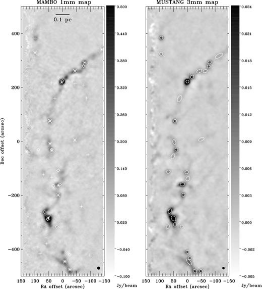
MAMBO (left) and MUSTANG (right) maps of OMC 2/3. The MAMBO map has been spatially filtered to recover only those scales to which the MUSTANG map is sensitive. Both maps have units of Jy pixel−1 with 11 arcsec × 11 arcsec pixels. In the 1 mm map, plus signs show the locations of starless cores (Sadavoy et al. 2010), asterisks show the positions of protostellar cores (Sadavoy et al. 2010), and diamonds show the locations of 3.6 cm continuum emission detected by Reipurth et al. (1999). In the map on the right, ellipses show the positions of structures identified using the getsources algorithm (Men'shchikov et al. 2012). The (0,0) position is (J2000) 05:35:23.35, −05:05:12.5.
MAMBO observations
The 1.2 mm continuum emission from OMC 2/3 was mapped with the Institute for Radio Astronomy in the Millimeter Range (IRAM) 30 m telescope at Pico Veleta, Spain, using the MAMBO array. Data were acquired between 1999 and 2002 and were reduced using the mopsi package following standard reduction steps. See Davis et al. (2009) for a more detailed description of the observations and analysis. The spatial scales recovered in the MAMBO map are greater than those of the MUSTANG map, a complexity that is discussed in Section 2.4. The noise in the MAMBO map is ∼8 mJy beam−1. The IRAM 30 m beam has been characterized at 1.3 mm by a Gaussian main beam (FWHM = 10.5 arcsec and amplitude 0.975), a Gaussian first error beam (FWHM = 125 arcsec and amplitude 0.005), and Gaussian second and third error beams with larger FWHM and lower amplitudes (Greve, Kramer & Wild 1998). Because the IRAM 30 m error beams have such small amplitudes relative to the main beam, we do not modify the 1.2 mm intensities as was done for the 3 mm map.
The observed 1.2 mm emission map is also shown in Fig. 1. The 3 and 1 mm emission maps look qualitatively very similar, as expected if thermal dust emission on the Rayleigh–Jeans tail is the dominant emission mechanism.
Ammonia observations
The NH3 (1,1) and (2,2) lines were observed towards OMC 2/3 by the Very Large Array (VLA) and the GBT. Details of the observations and calibration are given in Li et al. (2013). The combined VLA and GBT map has a spatial resolution of ∼5 arcsec and a spectral resolution of 0.6 km s−1. The kinetic temperature of the gas was derived in Li et al. (2013) following the procedures outlined in Li, Goldsmith & Menten (2003) and Ho & Townes (1983).
In this paper, the temperature at each position is determined from a smoothed and regridded Tgas map from Li et al. (2013), putting it on the same ∼11 arcsec resolution grid of the 1.2 and 3.3 mm continuum maps. Any position included in the continuum maps but not included in the NH3 maps was assigned the median temperature value of the map (16.5 K). The range of temperatures in this analysis (12 ≤ T ≤ 20) is relatively narrow, so an assumed value of 16.5 K will not be too far off the true line-of-sight average temperature for any region in OMC 2/3. Roughly 4 per cent of the pixels in our analysis were assigned the median temperature value of 16.5 K. For our analysis, we assume that the gas and dust temperatures are coupled, a valid assumption for densities greater than 104 cm−3 (Doty & Neufeld 1997; Goldsmith 2001). The dust temperature map thus derived is shown in Fig. 2.
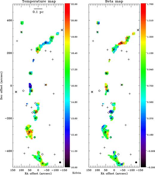
Temperature (left) and emissivity spectral index (right) maps of OMC 2/3. The temperature map comes from Li et al. (2013) and is smoothed and regridded to the 11 arcsec resolution of the 1 and 3 mm continuum maps. Temperature is only plotted where the emissivity spectral index is calculated. The emissivity spectral index in each pixel is derived from the ratio of the 1 to 3 mm fluxes, using the respective temperature map values as the isothermal temperature along the line of sight. See Sections 3.1 and 4.6 for details. The symbols (plus signs, asterisks, and diamonds) are as in Fig. 1.
Spatial filtering
Ground-based bolometer maps all suffer from some degree of spatial filtering as part of the data reduction process, to remove significant atmospheric emission. The MUSTANG 3 mm map recovers less extended emission than the MAMBO 1 mm map, with spatial scales greater than ∼2.4 arcmin filtered out. We therefore pass the MAMBO data through the MUSTANG pipeline because the former have sensitivity to emission on larger scales than the latter. This operation ensures that the same spatial filtering is applied to both the 1 mm and the 3 mm observations. This technique is similar to that employed by Sadavoy et al. (2013) to compare Herschel and James Clerk Maxwell Telescope data. As a result of this filtering, the spectral indices determined in this paper are derived for the smaller scale material in the OMC 2/3 filament and cores and are not indicative of the more diffuse material in the OMC. In the relatively dense material traced by the MUSTANG observations, the gas and dust temperatures are expected to be well coupled (see Section 2.3). We smooth the MUSTANG 3 mm and NH3 temperature observations to the MAMBO resolution, and then we place all three maps on a common grid. We consider only those pixels with signal-to-noise greater than 10 in both the MAMBO map and the MUSTANG map.
ANALYSIS
Equation (1) assumes that the dust emission is optically thin, which may be a concern towards the peak of the dust SED but is of no concern for observations on the Rayleigh–Jeans tail of the SED. For instance, assuming standard dust-to-gas ratios and dust properties (Ossenkopf & Henning 1994), the 1.2 mm emission from a dense core with a V-band extinction of AV = 100 would have an optical depth of 0.004, while one would expect an optical depth of 0.1 for 350 μm emission. The assumption of optically thin emission at 1 and 3 mm is justified for the observations presented here.
The main assumptions required for equation (1) to reflect accurately the emission as a function of frequency are (1) a lack of free–free emission, (2) a lack of anomalous microwave emission (AME), and (3) a weak temperature dependence. We discuss these different cases in Section 4.
Spectral index map
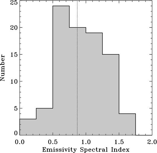
Histogram of the emissivity spectral indices measured in OMC 2/3. The vertical dashed line shows the median value of β. See Section 3.1 for details.
Getsources
The OMC 2/3 region has a complex background of filamentary structures that are not filtered out in our data (see Fig. 1). As such, source extraction algorithms that use intensity maxima and minima to identify structures (e.g. clumpfind; see Williams, de Geus & Blitz 1994) will include emission from these filaments in their extractions. Therefore, we identified sources using the getsources algorithm, which includes a prescription for filament extraction in addition to compact structures (see Men'shchikov et al. 2012 for details).
Briefly, getsources uses multiple spatial decompositions to identify structure over many scales and characterize source masks, which are defined by two-dimensional Gaussians. Information from the source masks (and filament masks) is combined over each wavelength to improve the final source footprint (i.e. in the case of blended sources at lower resolution) and to extract source properties. For efficiency, we masked out the edges of the 1 and 3 mm maps to avoid noisy regions (and false detections) associated with the low-coverage areas.
Using getsources version 1.140127, we identified initially 42 sources. This initial catalogue may include unreliable detections, e.g. due to the filtering. Therefore, we required all sources to be well detected in the single-scale decompositions (i.e. with significance > 1). Of the initial 42 sources, we rejected 12 for having either a low global significance or a low significance in either the 1 or 3 mm map. Table 1 gives the positions, sizes, and 3 mm fluxes associated with the 30 robust sources.
High-significance getsource objects.
| RA | Dec. | Major axisa | Minor axisa | Position anglea | Peak fluxa | Integrated fluxa |
|---|---|---|---|---|---|---|
| J2000 | J2000 | FWHM | FWHM | |||
| decimal (°) | decimal (°) | (arcsec) | (arcsec) | (° E of N) | (Jy beam−1) | (Jy) |
| 83.8473 | −5.0253 | 10.8 | 10.8 | 161.9 | 0.112 | 0.146 |
| 83.8613 | −5.1662 | 20.8 | 14.0 | 35.2 | 0.036 | 0.109 |
| 83.8650 | −5.1587 | 18.0 | 10.8 | 157.6 | 0.028 | 0.053 |
| 83.8522 | −5.1311 | 16.0 | 10.8 | 96.9 | 0.026 | 0.050 |
| 83.8584 | −5.0952 | 10.8 | 10.8 | 140.3 | 0.020 | 0.027 |
| 83.8599 | −5.0656 | 10.8 | 10.8 | 28.4 | 0.018 | 0.024 |
| 83.8427 | −5.0202 | 12.8 | 10.8 | 129.8 | 0.020 | 0.033 |
| 83.8513 | −5.1419 | 11.4 | 10.8 | 149.2 | 0.018 | 0.026 |
| 83.8250 | −5.0054 | 13.1 | 10.8 | 134.5 | 0.014 | 0.025 |
| 83.8472 | −5.2006 | 10.8 | 10.8 | 103.5 | 0.017 | 0.020 |
| 83.8338 | −5.2204 | 10.8 | 10.8 | 110.5 | 0.018 | 0.020 |
| 83.8736 | −4.9800 | 10.8 | 10.8 | 100.9 | 0.018 | 0.029 |
| 83.8397 | −5.2206 | 14.9 | 10.8 | 48.4 | 0.016 | 0.030 |
| 83.8259 | −5.0096 | 10.8 | 10.8 | 178.1 | 0.015 | 0.018 |
| 83.8598 | −5.1724 | 13.2 | 10.8 | 179.5 | 0.015 | 0.022 |
| 83.8353 | −5.0144 | 21.1 | 10.9 | 120.9 | 0.007 | 0.017 |
| 83.8449 | −5.2071 | 10.8 | 10.8 | 160.0 | 0.012 | 0.015 |
| 83.8480 | −5.1186 | 13.3 | 11.3 | 100.1 | 0.010 | 0.019 |
| 83.8456 | −5.2110 | 27.4 | 10.8 | 36.5 | 0.009 | 0.022 |
| 83.8605 | −5.0875 | 18.8 | 10.8 | 15.8 | 0.007 | 0.015 |
| 83.8530 | −5.1745 | 10.8 | 10.8 | 105.4 | 0.006 | 0.006 |
| 83.8736 | −4.9966 | 10.8 | 10.8 | 173.4 | 0.008 | 0.010 |
| 83.8294 | −5.0145 | 15.3 | 10.8 | 114.2 | 0.006 | 0.012 |
| 83.8664 | −5.1180 | 13.9 | 11.3 | 122.7 | 0.008 | 0.018 |
| 83.8670 | −5.1747 | 14.4 | 10.8 | 149.4 | 0.006 | 0.009 |
| 83.8469 | −5.1253 | 16.8 | 12.3 | 148.5 | 0.004 | 0.009 |
| 83.8619 | −5.1022 | 21.1 | 10.8 | 152.8 | 0.005 | 0.008 |
| 83.8156 | −4.9987 | 31.1 | 12.3 | 121.8 | 0.003 | 0.010 |
| 83.8552 | −5.0428 | 24.7 | 13.3 | 154.0 | 0.004 | 0.012 |
| 83.8333 | −5.0847 | 21.9 | 11.1 | 114.4 | 0.003 | 0.007 |
Note:aFrom the 3 mm flux map.
DISCUSSION
The median value of the emissivity spectral index between 1 and 3 mm in OMC 2/3 is β = 0.9, with a standard deviation of 0.3. The typical uncertainty due to noise in the spectral index at any given point in our map of β is 0.16. The systematic uncertainty in β due to absolute flux calibration uncertainties is 0.17.
The SED in OMC 2/3 is much shallower than has been measured in OMC 1, where 1.9 ≤ β ≤ 2.4 (Goldsmith et al. 1997). In the following, we discuss possible explanations for the low values of β determined in OMC 2/3.
Variations in β
The spectral indices ranged from β ≃ 1.9 to β ≃ −0.1 (note that a blackbody would have β = 0). This variation is significantly larger than the uncertainties in β, so the ratio of the 1 mm flux to 3 mm flux is strongly dependent on position.
We find no significant differences between the mean values of β found towards starless cores, protostellar cores, or at positions within the OMC 2/3 filament not associated with a core, with core positions taken from Sadavoy et al. (2010). The positions of possible protostars in OMC 2/3 (asterisks and diamonds in Fig. 2) correspond to regions with the full range of steep to shallow SEDs. There are relatively few points associated with starless cores and filamentary material removed from dense cores, but these regions also have the same average spectral index and spread (β ≃ 0.8-0.9 ± 0.3). One starless core in particular, J053530.0−045850 in the nomenclature of Sadavoy et al. (2010), is notable for its low-emissivity spectral index (β ≃ 0.6). We suggest that this core would be an interesting target for future observations.
Large grains
Values of emissivity spectral index with β < 1 have been seen before in the discs around pre-main-sequence stars and brown dwarfs (e.g. Lommen et al. 2007; Pérez et al. 2012; Ricci et al. 2012; Ubach et al. 2012) and are attributed to dust grain sizes up to millimetre scales. Seven dense cores in the Orion B9 region have had their spectral indices measured within 350 ≤ λ ≤ 850 μm, with a median value of β = 1.1 (Miettinen et al. 2012). Large grains provide a possible explanation for the relatively flat spectral index found in the Orion cores in the Miettinen et al. (2012) sample. The presence of millimetre-sized grains is also given as the likely explanation for β < 1 found in three Class 0 protostellar cores in the 1.3–2.7 mm wavelength range by Kwon et al. (2009).
Similarly, the low values of β in OMC 2/3 can be attributed to much larger dust grains than are typically found in the diffuse interstellar medium. The MUSTANG and MAMBO maps do not recover large-scale features associated with diffuse emission in OMC 2/3, so we have only measured the emissivity spectral index of the more compact (i.e. likely the densest) portions of the filaments as well as the dense starless and protostellar cores. Note that Johnstone & Bally (1999) find a typical density for this filament of ∼105 cm−3, much lower than is found in circumstellar discs but very similar to the densities found by Miettinen et al. (2012) in cores in Orion B9. In OMC 1, Goldsmith et al. (1997) find that the spectral index decreases with density, which is qualitatively consistent with the idea that the observations presented here of the densest portions of OMC 2/3 are characterized by a low average value of β.
Adopting the dust grain model presented in Ricci et al. (2010), we find that a spectral index of β ≃ 0.9 indicates that the maximum grain size is at least 1 mm and could be as large as 1 cm depending on the power-law slope of the dust grain size distribution. The dust opacity at 1 mm implied by the range of dust grain distributions and maximum grain size is 4 ≤ κ1 mm ≤ 10 cm2 g−1 (Ricci et al. 2010). This range of κ1 mm values is roughly a factor of 3–7 larger than the standard value given in Ossenkopf & Henning (1994, column 6 of table 1).
Free–free emission
In our determination of β (see Section 3.1), we assumed that there is no free–free emission contributing significantly to the observed 1 or 3 mm map. In regions of high-mass star formation, however, the 3 mm (and even 1 mm) continuum can have a significant contribution from free–free emission. For instance, towards Orion BN/KL in OMC 1 (to the immediate south of OMC 2/3), the 3 mm continuum is evenly split between free–free and thermal dust emission and in some places the continuum is actually dominated by free–free emission (Dicker et al. 2009). The OMC 2/3 region lacks the cluster of OB stars that dominate OMC 1, so we expect the 3 mm emission from OMC 2/3 to originate predominantly from dust rather than ionized gas. The expectation that the 3 mm emission is overwhelmingly from dust is borne out by the similar morphology of the MUSTANG and spatially filtered MAMBO maps (see Fig. 1). The assumption that the 3 mm continuum emission from OMC 2/3 is purely from dust emission has been made in previous studies (e.g. Shimajiri et al. 2009), and this assumption was also made in the recent MUSTANG survey of six Class 0 protostars (Shirley et al. 2011).
Reipurth, Rodríguez & Chini (1999) used the VLA to map the small-scale 3.6 cm emission towards OMC 2/3, finding 14 sources with flux densities ranging from 0.15 to 2.84 mJy at an angular resolution of 8 arcsec. For optically thin free–free emission (Sν ∝ ν−0.1), the contribution of any such emission to the MUSTANG map would be insignificant, given the ∼0.4 mJy beam−1 noise in the map. For optically thick emission, however, Sν ∝ ν2 and free–free emission becomes significant. We expect some localized emission at the positions of the OMC 2/3 protostars, which would bias our derived values of the emissivity spectral index to low values at these locations. The free–free emission measured by Reipurth et al. (1999) was unresolved in 11 of the 14 detected sources and less than 17 arcsec in all cases, so any free–free emission from these sources would be confined to regions one or two resolution elements wide in our maps. We suggest that the emissivity spectral index in regions with β < 0 is best explained by contamination from free–free emission towards these objects. For example, the few pixels in Fig. 2 with β < 0 generally correspond to known protostellar cores or the 3.6 cm continuum sources (as marked in Fig. 1). Nevertheless, we do not expect free–free emission on the spatial scales of filaments to be significant, and we see low values of β associated with such structures as well. The starless cores, protostellar cores, and the filament all have the same average value of β. Future observations of wavelengths between 3.3 mm and 3.6 cm would allow us to determine better the free–free contribution to the 3 mm map.
Anomalous microwave emission
In addition to thermal dust emission and free–free emission, AME can be another important component of the SED. A strong candidate for the source of AME is small, spinning dust grains (Draine & Lazarian 1998; Draine & Hensley 2012). The AME contribution to the total SED of molecular clouds has been estimated in a series of recent papers by the Planck Collaboration. In the Gould Belt molecular clouds, the AME typically peaks at 25.5 ± 0.6 GHz, falls below thermal dust emission at frequencies higher than ∼30–40 GHz, and is orders of magnitude smaller than thermal dust emission at frequencies greater than 80 GHz, where MUSTANG is sensitive (Planck Collaboration XII 2013a). In the Perseus molecular cloud, thermal dust emission dominates AME at frequencies greater than 60 GHz, and the AME contribution at 80 GHz and above is statistically insignificant (Planck Collaboration XX 2011). Similar results are found in the Milky Way Galactic plane (Planck Collaboration XXI 2011), and a wide range of Galactic clouds (Planck Collaboration XV 2014).
To estimate the contribution of AME to the observed 90 GHz emission, we use Planck data for OMC 2/3 acquired from the NASA IPAC Infrared Science Archive. The Planck resolution at 30 GHz (∼33 arcmin) is large enough to blend emission from OMC 1, which at long wavelengths is dominated by free–free emission, with the emission from OMC 2. We therefore restrict our analysis to Planck data between 30 and 353 GHz in the OMC 3 region. We find (see Fig. 4) that the emission falls by three orders of magnitude from 30 GHz (1 cm) to 70 GHz (4 mm). Therefore, emission at 100 GHz (3 mm) and higher frequencies should be dominated by thermal emission from large dust grains. We caution that the angular scales of the Planck maps (≥10 arcmin at frequencies ≤ 100 GHz) are much larger than the ∼10 arcsec angular scales probed by our MUSTANG and MAMBO observations. Nevertheless, we believe that there is not much contamination from AME in the MUSTANG 3 mm map. Higher angular resolution maps of 10–70 GHz continuum emission are needed, however, to confirm this expectation.
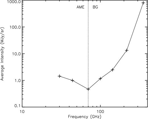
Planck spectrum of the OMC 3 region, from 30 to 353 GHz (see Section 4.4). At frequencies less than 70 GHz, AME dominates the SED. At frequencies greater than 70 GHz, thermal emission from big dust grains (labelled BG here) dominates the SED.
CO contamination
One final possible source of contamination in the 1 and 3 mm bands is molecular line emission. The main source of molecular line contamination of dust emission is from CO, the brightest molecular line in regions like OMC 2/3. For instance, Drabek et al. (2012) found that 12CO (3–2) emission contributes ≤20 per cent of the 850 μm flux observed with SCUBA-2 towards molecular clouds in most regions, but can be the dominant source of emission towards regions with molecular outflows. 12CO (1–0), at 115 GHz, falls outside the range of frequency range (81–99 GHz) to which MUSTANG is sensitive (Dicker et al. 2008). 12CO (2–1), at 230 GHz, falls within the MAMBO bandpass of 210–290 GHz (Bertoldi et al. 2007). Given the temperature and density distributions in OMC 2/3, we would expect an integrated intensity of CO (2–1) of ≤30 K km s−1 (van der Tak et al. 2007). This would contribute less than 2 mJy beam−1 to our 1 mm MAMBO map of OMC 2/3, which is much less than the noise in the map. An especially bright and broad (in velocity space) outflow could possibly make a significant contribution to the 1 mm map, artificially steepening the derived value of β in its vicinity. Over the majority of the OMC 2/3 filament, we do not expect molecular line contamination to significantly affect either the 3 or 1 mm continuum measurements of OMC 2/3.
Line-of-sight temperature variations
In the Rayleigh–Jeans approximation (hν ≪ kT), the observed flux at a given frequency is linearly dependent on temperature, so the ratio of fluxes at different frequencies is independent of temperature. The Rayleigh–Jeans approximation is only loosely valid for our observations of the OMC 2/3 region, with hν/k values of 12 and 4 K at 250 and 90 GHz, respectively. Lis et al. (1998) found that the temperatures of cores within OMC 2/3 are roughly 17 K, with evidence for warmer (∼25 K) dust in the filament. The gas kinetic temperature of the OMC 2/3 filament was measured using GBT and VLA observations of the NH3 (1,1) and (2,2) inversion transitions (Li et al. 2013). The gas temperatures are found to be mostly in the range of 10 ≤ Tgas ≤ 20 K. We therefore consider the possibility that line-of-sight temperature variations influence the values of β determined from the cold dust in OMC 2/3.
When determining the emissivity spectral index map shown in Fig. 2, we assumed that the temperature along each line of sight is constant. The true temperature distribution along each line of sight is very likely to be variable, so here we estimate the importance of line-of-sight temperature variations on our β map. We construct a toy model where the dust temperature along a line of sight is given by a Gaussian distribution with a 1σ width of 25 per cent of the mean temperature. We let the mean temperature vary from 5 to 25 K in steps of 0.1 K. For each distribution, we calculate the ratio of the continuum emission at 1.1 and 3 mm, assuming an emissivity spectral index of 1. The 1 mm/3 mm flux ratio depends on the temperature distribution of the dust, especially for low temperatures where the Rayleigh–Jeans approximation is least valid. We then use equation (4) to determine the emissivity spectral index that would be derived from the 1 mm/3 mm flux ratio. We find that temperature variations lead to a small overestimate of the emissivity spectral index, i.e. temperature variations along the line of sight push β to larger absolute values. The error is 2 per cent (or less) for temperature distributions centred on 10 K or warmer, and increases to 8 per cent at a mean temperature of 5 K (see Fig. 5). We therefore find that line-of-sight temperature variations could systematically bias our derived values of β, but at a level much lower than the uncertainties introduced by noise and absolute flux calibration errors. The systematic bias due to line-of-sight temperature variations moves β in the opposite direction of our surprising result – i.e. we find that the SED is shallower than predicted for dust in a filament while line-of-sight temperature variations work to steepen the SED.
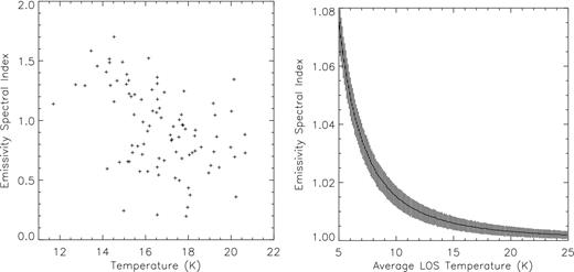
Left: plot of the emissivity spectral index derived from 1 and 3 mm continuum observations plotted against the temperature derived from NH3 (1,1) and (2,2) observations. Each data point is an independent pixel in the maps in Fig. 2. Right: results of Monte Carlo simulations of the emissivity spectral index that would be derived from 1 and 3 mm flux measurements of dust with a range of temperatures along the line of sight, plotted against the average line-of-sight temperature. The dust has an intrinsic emissivity spectral index of β = 1 and the line-of-sight temperature follows a Gaussian distribution with a width of 25 per cent of the mean temperature. The curving black line shows the mean β that would be determined and the vertical lines show the 1σ variation around the mean.
Fig. 5 compares β and temperature for the entire OMC 2/3 region. We find that β and Td are anticorrelated at the 4σ level. An anticorrelation between temperature and the emissivity spectral index has been seen previously in some molecular clouds (e.g. Dupac et al. 2003; Juvela et al. 2013), but other studies have not found conclusive evidence for a temperature-dependent emissivity spectral index (e.g. Veneziani et al. 2013). When using dust emission maps to determine both the temperature and emissivity spectral index, line-of-sight temperature variations can create spurious Td–β correlations (e.g. Shetty et al. 2009a,b; Schnee et al. 2010; Malinen et al. 2011; Juvela & Ysard 2012a,b; Ysard et al. 2012), though these can be at least partially overcome by careful analysis and statistical modelling (e.g. Kelly et al. 2012; Juvela et al. 2013). The analysis here is different from most previous studies of correlations between temperature and β in that these two quantities are determined from different data sets (NH3 observations and millimetre wavelength dust emission). As shown in Fig. 5, this anticorrelation, if real, is not caused by line-of-sight temperature variations.
SED shape
It is possible that our assumption of a power-law dust emissivity (i.e. κν ∝ νβ) between 90 and 250 GHz is not justified. For certain size distributions and compositions, detailed models of the dust opacity between 90 and 250 GHz show that it has a more complicated form (e.g. Draine 2006). Laboratory measurements and theoretical models of dust grain analogues have found that the emissivity can be temperature dependent (e.g. Agladze et al. 1996; Boudet et al. 2005; Meny et al. 2007) and not well described by a simple power law (e.g. Coupeaud et al. 2011; Paradis et al. 2011). The relatively low values of β we find might not be a result of large dust grains, but rather may be determined by the grain composition, temperature, and the wavelengths of our observations. Observations of circumstellar discs, however, often sample the SED from sub-millimetre to centimetre wavelengths and these are successfully modelled with a simple power-law opacity (e.g. Lommen et al. 2007; Pérez et al. 2012).
Calibration errors
A trivial explanation for the low values of β found in OMC 2/3 would have calibration errors. Given the relatively large frequency range between the MAMBO and MUSTANG observations, it would require a large error in the flux calibration to bring the emissivity spectral index into agreement with values found in Perseus B1 or the Orion nebula cluster. For instance, if we decrease the fluxes in the 3 mm map by 10 per cent and increase the fluxes in the 1 mm map by 10 per cent, then the median value of β increases from 0.9 to 1.0 (the standard deviation of derived values of β remains 0.3). To bring the median value of β up to 2, we would need to increase the ratio of S250 GHz/S90 GHz by a factor of 4. We do not believe that the flux uncertainties in the MAMBO or MUSTANG maps are anywhere near that high, so the absolute calibration of the bolometer maps is not likely to be the main driver of the low values of β found here.
Interpretation
Of the possible explanations for the shallow emissivity spectral index in OMC 2/3, we find that the two most likely are the presence of large grains or a dust emissivity not well described by a single power law. If dust grains in OMC 2/3 are characterized by millimetre-sized scales, this would be the first report of such large grains in structures with scales of the order of 1 pc. The protostellar cores and circumstellar discs with millimetre-sized grains have sizes of |$\lessapprox$|0.1 pc. It could be important to models of grain growth in discs and cores if the dust in filaments is already quite large. In this case, it will be important to determine if OMC 2/3 is unique in exhibiting large grains or if this is a common feature of star-forming filaments. Although OMC 2/3 is unique in that it has a higher density of starless and protostellar cores than other regions within ∼500 pc of the Sun, there are no other properties (mass, density, temperature, etc.) that would lead one to suspect that the dust grains in OMC 2/3 ought to have properties significantly different from those found in other nearby molecular clouds.
Alternatively, the shallow spectral index between 1 and 3 mm found in OMC 2/3 is due to an SED that is not well characterized by a power-law function at millimetre wavelengths. In this case, the grains are not necessarily larger than that are commonly found in nearby molecular clouds. It would be important to take the true shape of the dust emissivity into account when conducting future studies of β in filaments. In either case, more detailed observations are needed to study the full dust SED in filaments to make accurate measurements of mass, temperature, and possible large grains.
FUTURE WORK
Some of the assumptions made in Section 3 and some of the potential sources of error given in Section 4 can be tested with additional observations.
We have made the assumption that all of the 3 mm flux comes from dust emission, but it seems clear that free–free emission may contribute somewhat to the observed 3 mm map, especially near protostars. The contribution of free–free emission to the 3 mm map can be tested by making observations at wavelengths between the 3.6 cm map produced by Reipurth et al. (1999) and the 3.3 mm map shown here. These observations could be used to determine at what wavelength the free–free emission observed by Reipurth et al. (1999) switches from being optically thick to thin, allowing us to subtract accurately the free–free component from the 3 mm map and make a more accurate map of the emissivity spectral index.
We have made the assumption that the dust opacity is given by a power law, but this assumption can be tested by additional observations. To avoid uncertainties introduced by line-of-sight temperature variations, observations at 850 μm (with SCUBA-2, for example) or 2 mm (with the IRAM 30 m, for example) could be used to constrain better the shape of the (sub)millimetre SED and minimize the effect of uncertainties in absolute flux calibration on the derived value of the emissivity spectral index. Herschel observations between 70 and 500 μm could also be folded into this analysis, with similar spatial filtering and careful corrections for temperature variations and optical depth. High-resolution extinction maps could also be used to constrain the dust opacity independently from the dust temperature distribution.
SUMMARY
We have mapped the emissivity spectral index of the OMC 2/3 using new 3 mm observations paired with previously published observations of the 1 mm continuum and NH3-derived gas temperature. Focusing more on spatial scales of filaments and cores, we find that the emissivity spectral index is much shallower than is often assumed for dust in molecular clouds, with β = 0.9 ± 0.3. We find a weak correlation between β and Td, though there are no significant differences between the average values of β found in the OMC 2/3 filament, in the starless cores, and in the protostellar cores. Such a low average value of β in OMC 2/3 could be explained by millimetre-sized dust grains, as inferred in many circumstellar discs. Dust emissivities that vary with temperature or opacities that do not vary with wavelength as a simple power law could also explain our observations. We do not expect either free–free emission or AME to be significant on the scale of the 2-pc-long OMC 2/3 filament, though, if present and sufficiently bright, either emission mechanism would result in lower absolute values of β. We suggest future observations that can be used to determine the strength of free–free emission and AME.
We thank our anonymous referee for comments that improved the content and clarity of this paper. The National Radio Astronomy Observatory is a facility of the National Science Foundation operated under cooperative agreement by Associated Universities, Inc. JDF acknowledges support by the National Research Council of Canada and the Natural Sciences and Engineering Council of Canada(NSERC) via a Discovery Grant. RF is a Dunlap Fellow at the Dunlap Institute for Astronomy and Astrophysics, University of Toronto. The Dunlap Institute is funded through an endowment established by the David Dunlap family and the University of Toronto. DL is supported by China Ministry of Science and Technology under State Key Development Programme for Basic Research (2012CB821800). We would also like to thank the MUSTANG instrument team from the University of Pennsylvania, NRAO, Cardiff University, NASA-GSFC, and NIST for their efforts on the instrument and software that have made this work possible. DL acknowledges the support from National Basic Research Programme of China (973 programme) No. 2012CB821800, NSFC No. 11373038, and Chinese Academy of Sciences Grant No. XDB09000000.
Facilities: GBT, VLA, IRAM 30 m
