


Abstract
We describe the structural and kinematic properties of the first compact stellar systems discovered by the Archive of Intermediate Mass Stellar Systems project. These spectroscopically confirmed objects have sizes (∼6 < Re [pc] < 500) and masses (∼2 × 10⁶ < M*/M⊙ < 6 × 10⁹) spanning the range of massive globular clusters, ultracompact dwarfs (UCDs) and compact elliptical galaxies (cEs), completely filling the gap between star clusters and galaxies. Several objects are close analogues to the prototypical cE, M32. These objects, which are more massive than previously discovered UCDs of the same size, further call into question the existence of a tight mass–size trend for compact stellar systems, while simultaneously strengthening the case for a universal ‘zone of avoidance’ for dynamically hot stellar systems in the mass–size plane. Overall, we argue that there are two classes of compact stellar systems (1) massive star clusters and (2) a population closely related to galaxies. Our data provide indications for a further division of the galaxy-type UCD/cE population into two groups, one population that we associate with objects formed by the stripping of nucleated dwarf galaxies, and a second population that formed through the stripping of bulged galaxies or are lower mass analogues of classical ellipticals. We find compact stellar systems around galaxies in low- to high-density environments, demonstrating that the physical processes responsible for forming them do not only operate in the densest clusters.
1 INTRODUCTION
In the past 15 years there has been a revolution in the study of low-mass stellar systems. It began with the discovery (Hilker et al. 1999; Drinkwater et al. 2000) in the Fornax cluster of a population of generally old and compact objects with luminosity/mass and size intermediate between those of globular clusters (GCs) and the few then-known compact elliptical galaxies (cEs). These objects, known as ultracompact dwarfs (UCDs; Phillipps et al. 2001), became the first in a series of stellar systems found to exist with properties between star clusters and galaxies. They were followed by a zoo of objects inhabiting slightly different regions of the size–luminosity parameter space. These new objects included extended star clusters such as ‘Faint Fuzzies’ (Larsen & Brodie 2000, 2002) and ‘Extended Clusters’ (Huxor et al. 2005, 2011a; Brodie et al. 2011; Forbes et al. 2013), additional Milky Way (MW) and M31 dwarf spheroidals and ultrafaint dwarf galaxies (e.g. Willman et al. 2005; Zucker et al. 2006, 2007; Belokurov et al. 2007), and a host of new cEs (Mieske et al. 2005; Chilingarian et al. 2007; Smith Castelli et al. 2008; Chilingarian et al. 2009; Price et al. 2009) that fill the gap between M32 and ‘normal’ elliptical galaxies.
These discoveries have broken the simple division thought to exist between star clusters and galaxies, with UCDs displaying properties that lie between those of ‘classical’ GCs and early-type galaxies. Naturally, this situation has led to a search for unifying scaling relations, and therefore formation scenarios, for the various compact stellar systems (CSSs) and early-type galaxy populations.
Initial indications of a tight mass–size relation for the UCD and cE populations that extend from the massive GC (i.e. stellar mass >2 × 10⁶ M⊙) to elliptical galaxy regime (Haşegan et al. 2005; Kissler-Patig, Jordán & Bastian 2006; Dabringhausen, Hilker & Kroupa 2008; Murray 2009; Misgeld & Hilker 2011; Norris & Kannappan 2011) have been called into question by the discovery of extended but faint star clusters that broaden the previously observed tight relation for UCDs at fainter magnitudes (see e.g. Brodie et al. 2011; Forbes et al. 2013). Investigating the reality of such trends requires a more systematic and homogeneous sample of CSSs than currently exists.
In this paper series, we present the archive of intermediate mass stellar systems (AIMSS) survey. The goal of this survey is to produce a comprehensive catalogue of spectroscopically confirmed CSSs of all types which have resolved sizes from Hubble Space Telescope (HST) photometry, as well as homogeneous stellar mass estimates, spectroscopically determined velocity dispersions, and stellar population information. This catalogue will then be used to systematically investigate the formation of CSSs and their relationships with other stellar systems.
In order to achieve this goal, we have undertaken a search of all available archival HST images to find CSS candidates. We have deliberately broadened the selection limits traditionally used to find CSSs, both to probe the limits of CSS formation and to avoid producing spurious trends in CSS properties. One of the first results of the AIMSS survey presented in this paper is the discovery of further examples of a class of extremely dense stellar systems which broaden the previously suggested mass/luminosity–size trend to brighter magnitudes.
The AIMSS survey also includes a key additional parameter – central velocity dispersion. The central velocity dispersion of stars has been shown to be one of the best predictors of galaxy properties (e.g. Forbes & Ponman 1999; Cappellari et al. 2006; Graves, Faber & Schiavon 2009). It can also provide clues to the evolutionary history of a galaxy since, for example, tidal stripping will tend to reduce both the size and luminosity of a galaxy but its velocity dispersion will remain largely unchanged (see e.g. Bender, Burstein & Faber 1992; Chilingarian et al. 2009) and hence will remain a reliable signature of its past form.
In fact Chilingarian et al. (2009) showed that when their simulated disc galaxy on a circular orbit around a cluster potential is stripped severely enough to lose ∼75 per cent of its original mass, the global velocity dispersion is essentially unaffected (their fig. 1). This is because as stripping progresses it is increasingly the tightly bound central stellar structure (either nucleus or bulge) that comes to dominate the global light distribution of the galaxy, and the dispersion of this is relatively unaffected by the loss of an outer dark matter halo. The central velocity dispersion, which is always dominated by the stellar component of the galaxy, is likely to be less affected by stripping, at least until the point where the central mass component itself begins to lose mass.
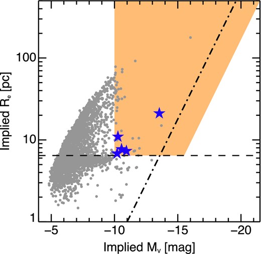
Implied luminosity–size plot for objects detected in an HST ACS pointing centred on NGC 4649, created assuming that all objects detected are at the same distance as NGC 4649. The grey dots are all objects detected by SExtractor in the ACS image. The shaded region indicates the selection region, the dashed horizontal line is the HST resolution limit at the distance of NGC 4649. The dot–dashed line shows the edge of the ‘zone of avoidance’ for early-type galaxies and CSSs (see Section 5.3). The selection region extends to 1.5 mag beyond the edge of the ‘zone of avoidance’ to ensure that we do not reject genuinely CSSs. The large blue stars are those objects which meet the selection criteria (including the ellipticity limit and a visual check for obvious artefacts/background galaxies) and are therefore suitable for spectroscopic follow-up.
Although the number of objects with sizes and luminosities intermediate between those classified as UCDs and cEs has grown substantially over the last few years, the number with measured velocity dispersions has not kept pace. In the compilation of Forbes et al. (2008), there were only two objects shown in their plot of velocity dispersion against luminosity in the gap between UCDs and cEs. Here we present velocity dispersions for 20 objects, many of which lie in this gap.
In the current paper, we present the catalogue of properties, and examine the mass–size, mass–surface mass density, and mass–σ behaviour of the first 28 (20 of which have velocity dispersion measurements) of our objects to be spectroscopically confirmed. In future papers in this series, we will examine the dynamics, stellar populations, and mass-to-light ratios of CSSs in more detail. An additional paper will provide the full photometric catalogue of candidate CSSs.
2 SAMPLE
2.1 AIMSS target selection
Our experience with the pilot programme of this survey (Norris & Kannappan 2011) demonstrated that inferred effective radii and absolute magnitudes (both determined by assuming physical association between the candidate CSS and an adjacent, larger galaxy), when combined with the existence of a hard edge in the luminosity–size distribution of CSSs (as seen in Brodie et al. 2011; Misgeld & Hilker 2011; Norris & Kannappan 2011) can be used to reliably select CSSs for spectroscopic follow up.
In this project, we select CSS candidates using the following procedure.
We first search the Hyperleda catalogue (Paturel et al. 2003)1 to find all galaxies with recessional velocity between 500 and 14 000 km s−1 (∼7–200 Mpc assuming H0 = 70 km s−1 Mpc−1) with MB < −15. Given the resolution of the HST, this distance limit ensures that CSSs of effective radius >50 pc will be adequately resolved in any available HST images.
We then search the HST archive2 for suitable Wide Field Planetary Camera 2 (WFPC2), ACS, and WFC3 broad-band optical images (i.e. exposures in the W or LP filters with exposure times >50 s, and at least two subexposures to allow adequate cosmic ray removal) located within 150 kpc in projection of all the selected galaxies (only 9 out of 813 objects from the extended cluster/UCD catalogue of Brüns & Kroupa 2012 are located beyond 150 kpc from their host galaxy). This limitation is simply to ensure that we can safely make the necessary assumption that CSSs and the host galaxy (of known distance) are physically associated. This necessarily means that isolated CSSs like the one discovered by Huxor, Phillipps & Price (2013) are unlikely to be discovered by our approach.
Suitable drizzled frames are then downloaded from the HST archive and analysed using SExtractor (Bertin & Arnouts 1996). SExtractor is used to produce a list of detected objects, their apparent magnitudes, a first estimate of their effective radii, and CLASS|$\_$|STAR (star–galaxy separation parameter) values. The principle benefits of using SExtractor to examine the images are the speed of the process and the reliability of the star–galaxy classification, which allows reliable rejection of unresolved objects without the need to individually fit surface brightness profiles for each object in the image. The principle limitation of using SExtractor is in the way backgrounds are subtracted: if the BACK|$\_$|SIZE parameter is too large CSSs located close to bright galaxies are lost, where BACK|$\_$|SIZE is set too small then the CSSs are themselves oversubtracted leading to systematically reduced effective radii estimates. We have optimized the choice of BACK|$\_$|SIZE using HST imaging of known CSSs as a training set, finding that a BACK|$\_$|SIZE of 64 is optimal for ACS images and 32 for WFPC2.
The SExtractor catalogues produced from different pointings and instruments are then combined, with overlapping magnitude estimates (e.g. from overlapping pointings with WFPC2 and ACS) averaged with error weighting. For any particular filter where overlap occurs between instruments, ACS size estimates are preferred to WFPC2, and WFC3 is preferred to both ACS and WFPC2.
The photometry of every detected object is corrected for Galactic extinction (following Schlafly & Finkbeiner 2011) and then converted into an absolute magnitude assuming every object is located at the distance of the main galaxy. Likewise the size estimates are converted into physical units.
A version of Fig. 1 is produced for each filter available. Using the properties of known CSSs (from our master catalogue described in Section 2.2) as a training set, a conservative region containing the rough mass–size trend of CSSs is then selected. This selection region extends 1.5 mag beyond the approximate edge of the previously known CSS population to ensure that we do not reject genuinely more compact objects. Objects which lie within this region, are relatively round (ϵ < 0.25), and have spatially resolved effective radii, are retained for further study. If subsequently spectroscopically confirmed, these first-pass estimates of the physical properties of the objects are refined using more sophisticated methods (see Section 3.5.1).
We apply no colour cuts, thereby avoiding discarding potentially interesting objects that could be young and blue, or dusty and red, such as the young massive clusters (YMCs) of NGC 34 and NGC 7252.
The remaining candidates are then examined individually by eye and any remaining spurious (due to artefacts, obvious background galaxies, etc.) candidates removed. Candidates are then cross-matched with literature compilations to prevent reobservation of previously known targets.
Although we make every effort to be as complete as possible, there are particular situations where our photometric completeness is likely to be severely reduced. A first obvious case is for objects projected close to the central regions of bright galaxies, where the high (and quickly varying) galaxy background is difficult to subtract cleanly in an automated manner. A more subtle example is for objects associated with spiral galaxies. In this case, the irregular galaxy light distribution makes reliably detecting CSSs projected on to the face of the disc extremely challenging. Only in cases of edge-on spiral galaxies do we expect to reliably detect CSSs associated with spirals. It is also the case that our selection region could also potentially reject the youngest and most luminous YMCs, which if they are sufficiently massive and young (but not enshrouded by dust) could lie more than 1.5 mag into the ‘zone of avoidance’ (see Section 5.3) for old stellar systems. Finally, in cases of galaxy mergers, the complex light distributions mean that there will be significant spatial variations of CSS detection efficiency.
The CSS candidates were then targeted for spectroscopic confirmation, principally at the SOAR and Keck telescopes. As these spectra were generally obtained during twilight or as filler targets, the objects for which spectra were obtained were generally brighter targets (V = 21.5 is the practical limit) selected randomly based on the current airmass (Table 1).
CSSs spectroscopically confirmed by the AIMSS collaboration. The setup column describes the instrument (GS = Goodman Spectrograph, GM-S = GMOS South, DM = DEIMOS), grating (l mm−1), slit width, total exposure time and resulting FWHM spectral resolution in Å, and seeing in arcseconds.
| Name | RA | Dec. | Date | Telescope | Setup | Vhelio |
|---|---|---|---|---|---|---|
| (J2000) | (J2000) | (dd/mm/yy) | (km s−1) | |||
| NGC 0524-AIMSS1 | 01:24:45.6 | +09:33:26.1 | 14/08/10 | SOAR | GS 1200 1.68 arcsec 4800 s 3.04 Å 0.9 arcsec | 2446 ± 18 |
| 09/11/10 | SOAR | GS 2100 0.84 arcsec 8400 s 0.92 Å 0.7 arcsec | 2525 ± 8 | |||
| NGC 0703-AIMSS1 | 01:52:41.1 | +36:10:14.4 | 20/10/12 | Keck | DM 1200 1.00 arcsec 716 s 1.55 Å 0.8 arcsec | 5685 ± 13 |
| NGC 0741-AIMSS1 | 01:56:21.3 | +05:37:46.8 | 12/01/13 | Keck | DM 1200 1.00 arcsec 960 s 1.55 Å 1.1 arcsec | 5243 ± 14 |
| NGC 0821-AIMSS1 | 02:08:20.7 | +10:59:26.6 | 23/10/06 | Keck | DM 1200 1.00 arcsec 3600 s 1.55 Å 1.0 arcsec | 1705 ± 6 |
| NGC 0821-AIMSS2 | 02:08:20.7 | +10:58:55.5 | 13/01/10 | Keck | DM 1200 1.00 arcsec 5400 s 1.55 Å 1.1 arcsec | 1480 ± 5 |
| NGC 0839-AIMSS1 | 02:09:40.6 | −10:11:07.1 | 07/11/12 | Keck | ESI 0.5 arcsec 1200 s 0.59 Å 0.7 arcsec | 3791 ± 34 |
| NGC 1128-AIMSS1 | 02:57:41.7 | +06:02:19.1 | 13/01/13 | Keck | DM 1200 1.00 arcsec 1200 s 1.55 Å 1.2 arcsec | 7320 ± 21 |
| NGC 1128-AIMSS2 | 02:57:44.5 | +06:02:02.2 | 13/01/13 | Keck | DM 1200 1.00 arcsec 1200 s 1.55 Å 1.2 arcsec | 7790 ± 13 |
| NGC 1132-UCD1 | 02:52:51.2 | −01:16:18.8 | 28/10/11 | SOAR | GS 2100 1.00 arcsec 3600 s 1.08 Å 1.0 arcsec | 7159 ± 27 |
| NGC 1172-AIMSS1 | 03:01:36.4 | −14:50:51.6 | 21/02/12 | Keck | DM 900 1.00 arcsec 600 s 2.2 Å 1.0 arcsec | 1743 ± 6 |
| NGC 1172-AIMSS2 | 03:01:34.4 | −14:49:50.7 | 21/02/12 | Keck | DM 900 1.00 arcsec 600 s 2.2 Å 1.0 arcsec | 1617 ± 15 |
| Perseus-UCD13 | 03:19:45.1 | +41:32:06.0 | 20/02/12 | Keck | DM 900 1.00 arcsec 4800 s 2.2 Å 1.0 arcsec | 5292 ± 14 |
| NGC 1316-AIMSS1 | 03:22:36.5 | −37:10:55.9 | 26/10/11 | SOAR | GS 2100 1.00 arcsec 4800 s 1.05 Å 0.8 arcsec | 1976 ± 12 |
| NGC 1316-AIMSS2 | 03:22:33.3 | −37:11:13.1 | 26/10/11 | SOAR | GS 2100 1.00 arcsec 4800 s 1.05 Å 0.8 arcsec | 1396 ± 13 |
| NGC 2768-AIMSS1 | 09:11:36.8 | +60:04:16.1 | 08/11/12 | Keck | ESI 0.5 arcsec 900 s 0.59 Å 0.8 arcsec | 1214 ± 20 |
| NGC 2832-AIMSS1 | 09:19:46.3 | +33:45:46.5 | 04/12/11 | Keck | DM 1200 1.00 arcsec 1.55 Å 1.0 arcsec | 6607 ± 20 |
| NGC 3115-AIMSS1 | 10:05:15.8 | −07:42:51.6 | 07/11/12 | Keck | ESI 0.5 arcsec 1800 s 0.59 Å 1.2 arcsec | 726 ± 19 |
| NGC 3268-AIMSS1 | 10:30:00.1 | −35:20:19.4 | 27-8/01/12 | SALT | RSS 2300 2.00 arcsec 3000 s 2.16 Å 1.5 arcsec | 2455 ± 57 |
| NGC 3923-UCD1 | 11:51:04.1 | −28:48:19.8 | 15/04/09 | SOAR | GS 600 1.5 arcsec 9600 s 6.2 Å 0.6 arcsec | 2097 ± 18a |
| 30/04/11 | Gemini-S | GM-S 1200 0.5 arcsec 10688 s 1.26 Å 0.9 arcsec | 2115 ± 30b | |||
| NGC 3923-UCD2 | 11:50:55.9 | −28:48:18.4 | 15/04/09 | SOAR | GS 600 1.5 arcsec 9600 s 6.2 Å 0.6 arcsec | 1501 ± 44a |
| 30/04/11 | Gemini-S | GM-S 1200 0.5 arcsec 10688 s 1.25 Å 0.9 arcsec | 1478 ± 29b | |||
| NGC 3923-UCD3 | 11:51:05.2 | −28:48:58.9 | 30/04/11 | Gemini-S | GM-S 1200 0.5 arcsec 10688 s 1.26 Å 0.9 arcsec | 2308 ± 35b |
| NGC 4350-AIMSS1 | 12:23:59.1 | +16:41:07.9 | 20/02/12 | Keck | DM 1200 1.0 arcsec 900 s 1.55 Å 0.9 arcsec | 1183 ± 8 |
| NGC 4546-UCD1 | 12:35:28.7 | −03:47:21.1 | 18/04/09 | SOAR | GS 600 1.68 arcsec 7200 s 6.3 Å 0.6 arcsec | 1256 ± 24a |
| 04/03/11 | SOAR | GS 2100 1.03 arcsec 3600 s 1.13 Å 1.2 arcsec | 1182 ± 2 | |||
| NGC 4565-AIMSS1 | 12:36:37.2 | +25:57:44.3 | 05/03/13 | Keck | ESI 0.5 arcsec 600 s 0.59 Å 1.0 arcsec | 1335 ± 9 |
| NGC 4621-AIMSS1 | 12:41:52.9 | +11:37:47.9 | 11/01/13 | Keck | DM 1200 1.00 arcsec 390 s 1.55 Å 0.8 arcsec | 474 ± 6 |
| M60-UCD1 | 12:43:36.0 | +11:32:04.6 | 11/01/12 | INT | IDS R300V 1.00 arcsec 1800 s 4.12 Å | 1236 ± 33 |
| 05/03/12 | SOAR | GS 2100 1.00 arcsec 3600 s 1.08 Å 1.0 arcsec | 1258 ± 11 | |||
| ESO 383-G076-AIMSS1 | 13:47:25.4 | −32:52:56.3 | 29/01/12 | SALT | RSS 2300 2.00 arcsec 1800 s 2.16 Å 1.0 arcsec | 11403 ± 24 |
| NGC 7014-AIMSS1 | 21:07:51.5 | −47:11:25.6 | 19/04/12 | SOAR | GS 2100 1.00 arcsec 3600 s 1.05 Å 0.7 arcsec | 5197 ± 14 |
| Contaminants | ||||||
| NGC 7418A-BG1 | 22:56:43.2 | −36:46:43.1 | 02/05/11 | SOAR | GS 2100 1.68 arcsec 3600 s 1.19 Å | 75300 ± 60 |
The net effect of the various selections, both in photometrically selecting targets, and in ensuring they were sufficiently luminous to spectroscopically confirm, is shown in Fig. 2. The two major limitations and their implications are (1) the necessity of resolving the objects in the HST imaging, meaning that the allowed effective radius increases with redshift, and (2) the V = 21.5 magnitude limit for spectroscopic followup, which means that only progressively brighter objects are found at higher redshift.
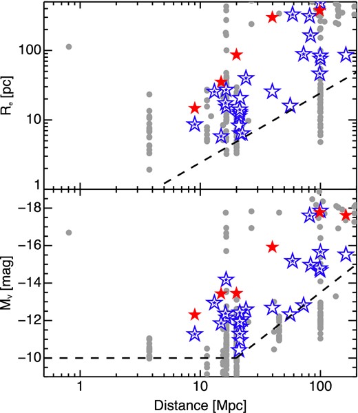
Upper panel: the effect of our requirement that objects must be resolved by the HST before we conduct spectroscopic follow up. The blue stars are our confirmed objects, the ones with filled stars inside denote the objects for which we were also able to obtain velocity dispersions. The red stars denote objects previously known which were observed as a comparison sample, all of which meet the same selections as the main AIMSS sample. The grey circles are literature GCs, UCDs and cEs. The dashed line shows the resolution limit of the HST with distance, assuming conservatively that to resolve an object, 2 times the effective radius must be larger than the HST resolution limit of 0.1 arcsec. Lower panel: the effect of our requirement that objects for spectroscopic follow-up must have MV < −10 and apparent V magnitude brighter than 21.5. The combination of the two requirements leads to the dashed line.
While conducting this project, several of our AIMSS targets were independently discovered and described by other authors (e.g. NGC 1132-UCD1; Madrid 2011; Madrid & Donzelli 2013, Perseus-UCD13; Penny, Forbes & Conselice 2012, M60-UCD1; Strader et al. 2013). In what follows, we make no distinction between these objects and the other AIMSS objects, as they were all selected using the above criteria and were analysed using the same methods.
2.2 Literature comparison samples
In addition to the AIMSS selected sample, we include several complementary literature samples that allow us to explore the properties of our objects relative to other CSSs and galaxy types.
It is our intention to provide the most comprehensive catalogue of CSS properties available. Therefore, we have attempted to include all spectroscopically confirmed UCDs and cEs in the literature which have available size measurements and which are more luminous than MV = −10. The principle literature sources for CSSs are the compilations of Misgeld & Hilker (2011) and Brodie et al. (2011) plus the recent update from Forbes et al. (2013), and to these compilations we add additional data for specific systems. Where possible we compile literature photometry for all objects and recompute their stellar masses using the same procedure as for our CSS sample (see Section 3.6). We note below those cases where this is not possible due to limited available photometry. The use of literature stellar masses ‘as is’ can obviously lead to systematic offsets in the stellar masses of some samples and/or object types. However, the magnitude of such offsets, for example, by using stellar masses derived using Kroupa instead of Salpeter initial mass functions (IMFs), is around 40 per cent which is small compared to the factor of 2–3 errors introduced by, for example, assuming a single old simple stellar population (SSP) versus a composite age stellar population. Therefore, we do not attempt to homogenize literature stellar mass estimates, especially as this process itself could lead to additional errors, in particular due to the observed variation of IMF with stellar mass (see e.g. Cappellari et al. 2013b).
To our knowledge, our compilation of 191 objects is the most comprehensive catalogue of GCs, UCDs, and cEs assembled to date for objects that have been spectroscopically confirmed, are more luminous than MV = −10, and have measured effective radii. The complete catalogue of CSSs and comparison samples are provided in Appendix A.
Throughout this paper, we will discuss the properties of the CSS sample in relation to the early-type galaxies in our sample. However, we fully expect that later type galaxies play an equally important role (possibly a dominant role in field/group environments) in the formation of certain types of CSS. We defer a detailed discussion of late-type galaxies in order to simplify the analysis, and in the belief that the behaviour of partially rotationally supported systems such as dEs/dS0s and S0s likely encapsulates much of the behaviour of later type systems without the added complications to analysis caused by ongoing star formation and internal dust.
2.2.1 dSph, dE and dS0 galaxies
We include literature data for a sample of dwarf spheroidals, dwarf ellipticals, and dwarf S0s to allow their comparison with our UCD and cE samples. Data on the MW and M31 dSph/dE systems come from Walker et al. (2009), McConnachie (2012), Tollerud et al. (2012, 2013), and references therein. Data on the dE/dS0 sample comes from Geha, Guhathakurta & van der Marel (2002, 2003), Chilingarian (2009), and Toloba et al. (2012) combined with five lower luminosity dwarf galaxies from Forbes et al. (2011). Where possible we add additional photometry for each source from the Sloan Digital Sky Survey (SDSS) DR9 (Ahn et al. 2012) corrected for foreground extinction following Schlafly & Finkbeiner (2011), in order to improve the subsequent determination of the stellar mass (see Section 3.6).
2.2.2 Nuclear star clusters
We make use of the compilations from Misgeld & Hilker (2011) and Brodie et al. (2011) to provide a comparison sample of dwarf galaxy nuclear star clusters.
2.2.3 Massive early-type galaxies
In order to examine the connection between UCDs/cEs and early-type galaxies (both ellipticals and S0s) we make use of the galaxy sample from Misgeld & Hilker (2011) and Brodie et al. (2011) combined with the ATLAS3D (Cappellari et al. 2011) survey to provide a representative comparison sample of normal early-type galaxies. Where galaxies are found in either Misgeld & Hilker (2011) or Brodie et al. (2011) and also in the ATLAS3D sample we prefer the ATLAS3D derived properties in our compilation.
We also take the effective radii and the total K-band magnitudes from Cappellari et al. (2011, originally from 2MASS). We then convert the K-band integrated magnitudes to V assuming V − K = 2.91, a colour that is appropriate for a stellar population with age = 10 Gyr and solar metallicity (Maraston 2005), and which should roughly match the stellar populations of the average elliptical galaxy. We derive stellar masses using the published stellar M/Lr values and r-band luminosity from Cappellari et al. (2013b), where the M/Lstars taken from Cappellari et al. (2013b) allows for some variation in the IMF between Kroupa and Salpeter (again, only a 40 per cent effect). The quoted central (Re/8) velocity dispersions are from Cappellari et al. (2013a).
2.2.4 Young massive clusters
In order to demonstrate the effects of age on the observed properties of CSSs, we include several YMCs found in recent galaxy mergers. Specifically, we include W3, W6, W26, and W30 from NGC 7252; S&S1 and S&S2 from NGC 34; and G114 from NGC 1316. These young objects are expected to fade over several Gyr to resemble UCDs (Maraston et al. 2004).
The data for the YMCs come mostly from the literature, although we spectroscopically reobserved W3 and W6 with SOAR as part of our calibration sample. The photometry and size estimates for the NGC 7252 clusters are from Bastian et al. (2013), those for the NGC 34 clusters are from Schweizer & Seitzer (2007), and the measurement for NGC 1316-G114 is from Bastian et al. (2006). In addition to the size estimates there are literature measurements for the velocity dispersions for NGC 7252 W3, W30, and NGC 1316 G114, which come from Maraston et al. (2004) and Bastian et al. (2006), respectively.
2.2.5 Globular clusters
We include the MV and Re values for MW GCs from Brodie et al. (2011) and add the measured central velocity dispersions of the clusters from Harris (1996) (2010 edition). We add the ‘extended but faint’ GCs from Forbes et al. (2013) and the M31 GCs from Strader, Caldwell & Seth (2011a), where we convert their measured MK to stellar mass assuming M/LK = 0.937, which is appropriate for a stellar population with age = 10 Gyr and [Fe/H] ∼ −0.8, when assuming a Kroupa IMF which better fits GCs than a Salpeter IMF (Strader et al. 2011a). The effect of changing [Fe/H] by ±0.5 only results in MK changing by 0.01 at this age (Maraston 2005). However, Strader et al. (2009, 2011a) observe that those M31 GCs with [Fe/H] < −1 have M/L relatively consistent with a Kroupa IMF, whereas nearly all M31 GCs with [Fe/H] > −1 have lower M/L than predicted from stellar population models with a Kroupa IMF. The most likely reason is that these GCs have a deficiency of low-mass stars with respect to the assumed IMF, although standard dynamical evolution (Kruijssen & Mieske 2009) does not appear to be a viable explanation for these observations. For our purpose, the main implication of assuming a fixed M/LK is that the stellar masses of some of the GCs could be in error by factors of 2 to 3. However, this does not affect any of the conclusions of the paper.
2.2.6 UCDs and cEs
We include additional UCDs from Norris & Kannappan (2011), Norris et al. (2012), and Mieske et al. (2013), as well as additional cEs from Chilingarian & Bergond (2010) and Huxor et al. (2011b, 2013). Where possible we take central velocity dispersions rather than aperture measurements.
3 OBSERVATIONAL METHODS
3.1 Spectroscopic observations
Tables 1 and 2 present the observing logs of objects observed to date as part of the AIMSS project. Table 1 shows those objects newly discovered or confirmed by this project, while Table 2 shows a sample of previously confirmed objects reobserved by us to provide a comparison/calibration sample. In both tables column 1 is a designation for the object, columns 2 and 3 are the right ascension and declination in J2000 coordinates, column 3 is the date of observation, column 4 lists the telescopes used to determine the objects redshift, column 5 provides the instrument setup used (instrument, grating, slit width, exposure time, and spectral resolution full width at half-maximum, FWHM), and column 6 gives the heliocentric recessional velocity and its error rounded to the nearest km s−1 measured using the procedure described in Section 3.3.
Previously confirmed CSSs and serendipitous objects (those observed in the same slit as AIMSS objects) with additional observations/analysis provided by the AIMSS collaboration.
| Name | RA | Dec. | Date | Telescope | Setup | Vhelio |
|---|---|---|---|---|---|---|
| (J2000) | (J2000) | (dd/mm/yy) | (km s−1) | |||
| Fornax-UCD3 | 03:38:54.0 | −35:33:34.0 | 31/10/10 | SOAR | GS 2100 1.5 arcsec 3600 s 1.36 Å 1.0 arcsec | 1473 ± 6 |
| NGC 2832-cE | 09:19:47.9 | +33:46:04.9 | 04/12/11 | Keck | DEIMOS 1200 1.00 arcsec 1.55 Å 1.0 arcsec | 7076 ± 9 |
| NGC 2892-AIMSS1 | 09:32:53.9 | +67:36:54.5 | SDSS | Spectrum from SDSS DR10 | 6847 ± 3 | |
| NGC 3268-cE1/FS90 192 | 10:30:05.1 | −35:20:32.0 | 27-8/01/12 | SALT | RSS 2300 2.00 arcsec 3000 s 2.16 Å 1.5 arcsec | 2479 ± 27 |
| Sombrero-UCD1 | 12:40:03.1 | −11:40:04.3 | 05/03/11 | SOAR | GS 2100 1.03 arcsec 2700 s 1.08 Å 1.1 arcsec | 1306 ± 6 |
| M59cO | 12:41:55.3 | +11:40:03.8 | 11/01/13 | Keck | DEIMOS 1200 1.00 arcsec 390 s 1.55 Å 1.0 arcsec | 703 ± 9 |
| ESO 383-G076-AIMSS2 | 13:47:25.3 | −32:53:09.9 | 29/01/12 | SALT | RSS 2300 2.00 arcsec 1800 s 2.16 Å 1.0 arcsec | 10978 ± 8 |
| NGC 7252-W3 | 22:20:43.7 | −24:40:38.0 | 30/05/11 | SOAR | GS 2100 1.03 arcsec 3600 s 1.05 Å 0.8 arcsec | 4744 ± 12 |
| NGC 7252-W6 | 22:20:44.0 | −24:40:27.7 | 30/05/11 | SOAR | GS 2100 1.03 arcsec 3600 s 1.05 Å 0.8 arcsec | 4606 ± 9 |
3.1.1 SOAR
The majority of our southern spectroscopic observations to date have been obtained using the Southern Astrophysical Research (SOAR) Telescope and the Goodman spectrograph (Clemens, Crain & Anderson 2004) in longslit and MOS modes. Our preferred setup with a 1 arcsec longslit and the 2100 l m−1 volume phase holographic (VPH) grating provides spectral resolution of FWHM ∼1 Å sampled at 0.33 Å with spectral coverage from 4850 to 5500 Å.
3.1.2 SALT
We used the South African Large Telescope (SALT) to observe fainter targets requiring exposure times impractically long to be used as filler targets for SOAR observing and which cannot be observed with Keck. The observations used the RSS spectrograph (Kobulnicky et al. 2003) with the 2300 l m−1 grating and a 2 arcsec wide longslit providing coverage from ∼4300 to 7400 Å with a spectral resolution (FWHM) of 2.16 Å, sampled with 0.7 Å pixels.
3.1.3 Gemini-South
As part of a study examining the GCs and UCDs of the shell elliptical NGC 3923 we obtained deep Gemini/GMOS spectroscopy of three UCDs (see Norris et al. 2012 for further details). The observations were made in MOS mode with the 1200 l m−1 grating and 0.5 arcsec slitlets, yielding spectra with a resolution of 1.26 Å FWHM and wavelength coverage from ∼4100 to 5600 Å. These observations were sufficiently deep to allow the measurement of velocity dispersions for all three UCDs.
3.1.4 Keck
The majority of our Northern hemisphere candidates were spectroscopically confirmed using the DEIMOS and ESI instruments on the Keck telescope (Sheinis et al. 2002; Faber et al. 2003). For DEIMOS our observational setup uses the 1200 grating, and a 1 arcsec wide longslit, centred on the calcium triplet region (∼8500 Å) providing a spectral resolution of 1.55 Å sampled at 0.32 Å. ESI gives a coverage from 3900 to 10900 Å and for our observations provides a spectral resolution of ∼0.59 Å when using a 0.5 arcsec wide longslit.
3.1.5 INT
We also obtained spectra of NGC 4649 UCD1 with the IDS instrument on the Isaac Newton Telescope using the RED+2 detector, the R300V grating, and a 1 arcsec longslit, providing a resolution of 4.12 Å FWHM over the whole visible spectrum.
3.2 Spectral reduction
Where available, our spectroscopic observations were reduced using the dedicated pipelines of the particular instruments used, e.g. using the Gemini-GMOS iraf package for GMOS observations as described in Norris et al. (2012).
In those cases where no dedicated pipeline currently exists, or it is insufficient for our purposes (i.e. for SOAR-Goodman, INT, and SALT-RSS spectroscopy), the observations were reduced using custom reduction pipelines. The pipelines used standard iraf routines to carry out bias and overscan subtraction, trimming of the science data to remove unnecessary spatial coverage, then flat fielding. Following flat fielding the idl implementation of la|$\_$|cosmic (van Dokkum 2001) was used to clean cosmic rays from each science exposure. iraf was then used to carry out wavelength calibration and rectification, as well as object tracing and extraction into a 1D spectrum (using apall) and finally combination of individual exposures (scombine).
3.3 Redshift determination and candidate confirmation
We measure the redshifts of all of our CSSs by cross-correlating the input spectra against a SSP spectral library (the high resolution, FWHM = 0.55 Å, ELODIE based models of Maraston & Strömbäck 2011) in the case of optical spectra, and a library of empirical stellar spectra observed with the same setup used for the Keck/DEIMOS CaT observations. The cross-correlation is carried out using the iraf task FXCOR in the rv package. More details regarding the estimation of errors and the procedure used to reject outlying velocities can be found in Norris & Kannappan (2011).
Because we have reobserved several of our objects with various telescope and instrument combinations, as well as reobserving several calibration objects, we are able to determine the repeatability of our recessional velocity determinations. Fig. 3 demonstrates that our velocity repeatability is generally very good, across the wide variety of telescope and instrument configurations which could lead to systematic differences between observations. The median difference between repeat measurements is 18 km s-1 with a dispersion of 45 km s−1 and all but two observations agree to within 3σ of their respective errors. The two significant outliers are the YMCs of NGC 7252 (W3 and W6) which are expected to be problematic due to their very young ages (∼300 Myr; Maraston et al. 2004) which can lead to significant template mismatch. We therefore believe that our recessional velocities are reliable at the ∼50 km s−1 level, which is sufficient to determine physical association between CSS candidate and host, but possibly not accurate enough for detailed analyses of correlated structures in position–velocity phase space (see e.g. Romanowsky et al. 2012).
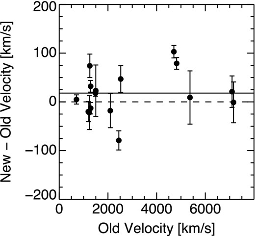
Our repeat/new recessional velocities compared to earlier AIMSS or literature velocities for a sample of 15 objects with repeat spectroscopic observations. The dashed line is the equality line, while the solid line shows the median of old–new velocities. The median offset is 18 km s−1, showing that our inhomogeneous spectroscopic observations are not systematically offset from previous measurements.
To confirm the nature of candidate objects we examine the difference in redshift between the CSS and the mean recessional velocity of the presumed host structure (i.e. galaxy, group, or cluster). Fig. 4 shows that only one AIMSS candidate found so far has a velocity offset greater than 550 km s−1 (except for one obvious high-z background object), which is similar to the largest velocity offset found for GCs in the GC system of the Sombrero galaxy (Bridges et al. 2007), and slightly lower than the 650 km s−1 maximum offset found for GCs of the group elliptical NGC 3923 (Norris et al. 2008, 2012).
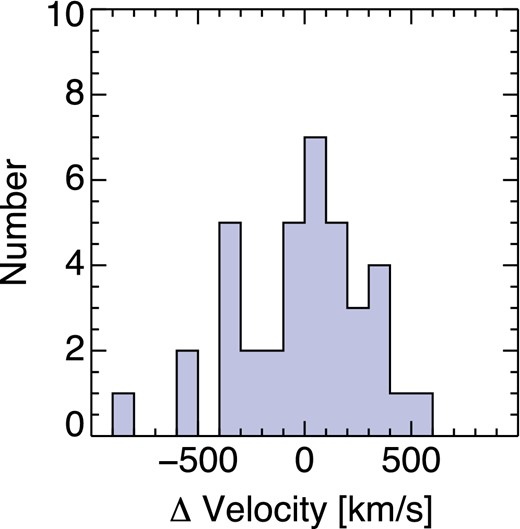
Histogram of the Δ velocities (CSS recessional velocity – host galaxy recessional velocity). The maximum velocity difference between CSS and presumed host is 849 km s−1 for the cE of NGC 1128, which resides in a medium sized group. From this plot, it can be seen that only the cE of NGC 1128 has a velocity offset larger than the largest velocity outlier in the GC system of the Sombrero galaxy (550 km s−1).
To produce a systematic recessional velocity offset limit we make use of the 2MASS All Sky Redshift Survey group catalogue of Crook et al. (2007) which is the most complete over the whole sky and which uses a luminosity function correction to account for galaxies which fall below the magnitude limit of the input redshift catalogue. Fig. 5 shows how we derive this limit. We start by plotting 3 times the velocity dispersion of the group/cluster versus the total number of galaxies in the structure for all 1604 groups in the Crook et al. (2007) low contrast group catalogue (red points). We then fit a relation to these groups for all structures with more than five members (to ensure a reliable dispersion measurement). For structures with less than five members we allow a maximum velocity offset of 550 km s−1 as found for the Sombrero galaxy GC system, which produces the dashed lines in the plot.
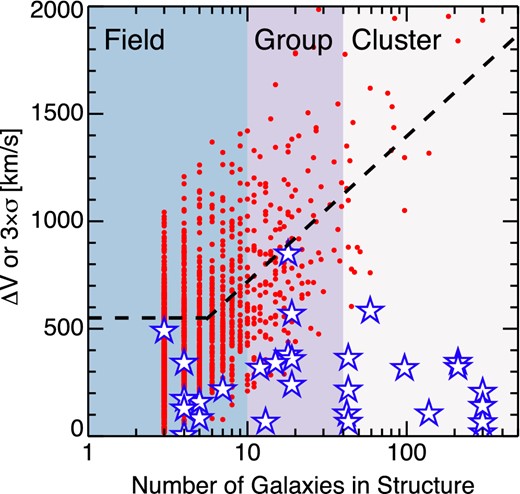
Absolute velocity offset of CSS from host galaxy, or 3 times the velocity dispersion of the group versus the number of galaxies in the group from the low-density contrast catalogue of Crook et al. (2007). The shaded regions display our adopted field/group/cluster classification. The blue stars are the velocity offset between our confirmed AIMSS objects and their host galaxies, in the case where their host galaxy is found in the Crook et al. (2007) catalogue. The red dots show 3 times the global (group/cluster) velocity dispersion of all groups found in the Crook et al. (2007) catalogue. They can be thought of as the largest velocity offset from the structure mean (a 3σ outlier) likely to be found for a galaxy within the bound structure. Hence CSS's selected to lie within this limit are likely to be bound to the structure they are projected on to. The dashed line is a fit to the red points for groups with more than five members; below this it is a fixed value of 550 km s−1 chosen to match the largest expected velocity outlier in the GC system of isolated mid-sized galaxies, such as the Sombrero galaxy. To date only one candidate (an obvious background galaxy with cz ∼ 75000 km s−1) has failed to lie below the dashed line and therefore to be physically associated with the assumed host galaxy. There is a noticeable absence of objects with velocity offsets above 400 km s−1 for larger structures (number of Galaxies >100). This may be an indication of the formation process; star cluster type objects will be expected to have velocities close to their host galaxies, but objects formed by stripping also must have velocities similar to those of the larger galaxies that did the stripping, as multiple close passes are required to do the necessary stripping.
Where the host galaxy of the AIMSS candidate lacks a counterpart in the Crook et al. (2007) catalogue we make use of literature determinations of environment and assume that environments classified as ‘field’ in the literature have 10 members, ‘groups’ have 40, and ‘clusters’ have 300. We then use the derived maximum velocity offsets for structures of these sizes as the appropriate limits. We have overplotted the absolute velocity offset for all AIMSS objects which have host galaxies in the Crook et al. (2007) catalogue as blue stars. As can be seen all but one (NGC 7418A-BG1 not plotted) of our candidate CSSs are found to be physically associated with the assumed structure, leading to a total success rate of 96 per cent.
3.4 Velocity dispersion determination
Integrated velocity dispersions (σ) for our CSSs were measured where the available spectra had sufficient resolution and S/N (generally >25 per Å was required to achieve reliable measurements), using version 4.65 of the penalized pixel fitting code (ppxf) of Cappellari & Emsellem (2004). This code fits each input spectrum with an optimal combination of template (the same SSP models and stellar templates as described in Section 3.3) spectra convolved with the line-of-sight velocity distribution (LOSVD).
Fig. 6 shows our σ measurements compared to literature measurements for five objects we reobserved as calibration objects. The one significant outlier is M59cO, where the literature value of 48 ± 5 km s−1 from Chilingarian & Mamon (2008) disagrees with ours (29.0 ± 2.5 km s−1) by almost 3 standard deviations. As our ppxf fit to this spectrum is excellent (see Fig. 7), and the resolution of our spectrum (23 km s−1 FWHM) is significantly below the measured value, we choose to adopt our value. In this case the offset is likely due to a combination of effects, including differences in seeing and slit/fibre width and positioning resulting in different spatial sampling and differences in the mix of templates used to fit the spectrum. In addition, the Chilingarian & Mamon (2008) value is derived from an SDSS spectrum and hence the resolution (of around 70 km s−1) is significantly higher than the measured velocity dispersion. Thus, this measurement is likely more uncertain than the quoted error would imply. All other repeat measurements are within the mutual 1σ errors, indicating that our measured velocity dispersions can be safely combined with other literature samples.
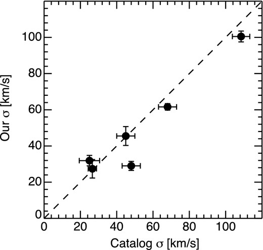
Our AIMSS velocity dispersion measurements compared to literature values for six objects which had previously been observed (from left-to-right; Sombrero-UCD1; Hau et al. 2009, Fornax-UCD3; Mieske et al. 2013, NGC 7252-W3; Maraston et al. 2004, M59cO; Chilingarian & Mamon 2008, M60-UCD1; Strader et al. 2013, NGC 2832-cE; Ahn et al. 2012). The significant outlier is M59cO (see Section 3.4). The dashed line is the equality relation.
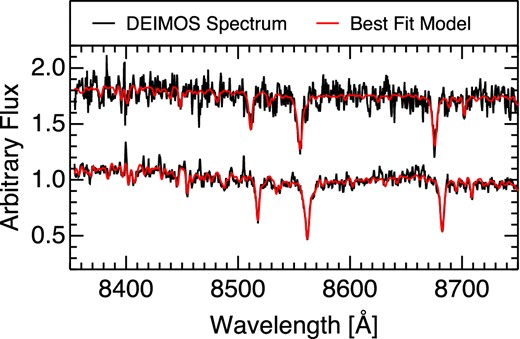
Our Keck/DEIMOS spectra for NGC 4621-AIMSS1 (upper black spectrum) and M59cO (lower black spectrum). The red lines in both cases are the best-fitting ppxf spectra. The actual flux values are arbitrary, with the NGC 4621-AIMSS1 spectrum offset for clarity. The quality of the spectra and the ppxf fits are evident in both cases.
As mentioned above, a complication of the velocity dispersion determination is that we are sensitive to only the light which falls within the instrument longslit. This means that for strongly peaked velocity dispersion profiles such as those measured for UCDs and cEs (e.g. Chilingarian & Bergond 2010; Frank et al. 2011), the velocity dispersion we have determined is, in fact, a luminosity-weighted average between the central velocity dispersion, and the true global average velocity dispersion of the CSS. Therefore, in order to properly estimate the dynamical mass of our sample it is first necessary to model the intrinsic light distribution of the CSS and then correct the measured velocity dispersion for the effects of slit losses and seeing. As the examination of the dynamical masses and mass-to-light ratios of our CSSs will take place in a forthcoming paper (Forbes et al., in preparation), we leave this additional analysis until then. For the current paper, we treat our measured velocity dispersions as approximations to the central velocity dispersions, and expect that they are correct to within 10 per cent of the final value (see e.g. Mieske et al. 2008a).
3.5 Photometric reanalysis
3.5.1 Effective radii
For those objects spectroscopically confirmed as CSSs, we use the available HST images to remeasure the effective radii using a range of techniques. We first subtract the host galaxy background. Where possible we use ELLIPSE in iraf to model the galaxy background and remove it, after masking other objects within the HST field of view. In those cases where the host galaxy background cannot be adequately modelled using ELLIPSE (e.g. where the centre of the host galaxy is not located on the image) we produce a median smoothed image following the procedure outlined in Norris & Kannappan (2011).
After background subtraction we use SExtractor to produce a size estimate as a first guess input for the ishape structural fitting code (Larsen 1999). We then use ishape to fit Sérsic and King models (with concentration 15, 30, 100, and unconstrained) to each object, using a point spread function (PSF) constructed using tinytim (Krist, Hook & Stoehr 2011). Where the best-fitting King or Sérsic model (as judged by the ishape χ2 value) has a radius less than 0.3 arcsec we accept this value as the correct major axis effective radius. For those cases where the best-fitting Sérsic or King model has a radius greater than 0.3 arcsec we use the SExtractor value, as this value is model independent and therefore potentially more resistant to under- or overfitting low surface brightness outer structures. Fig. 8 demonstrates that in the case where Re > 0.3 arcsec (which is 3 × the FWHM of the HST optical PSF) the ishape and SExtractor estimates are in good agreement, with a median offset of ∼4 per cent.
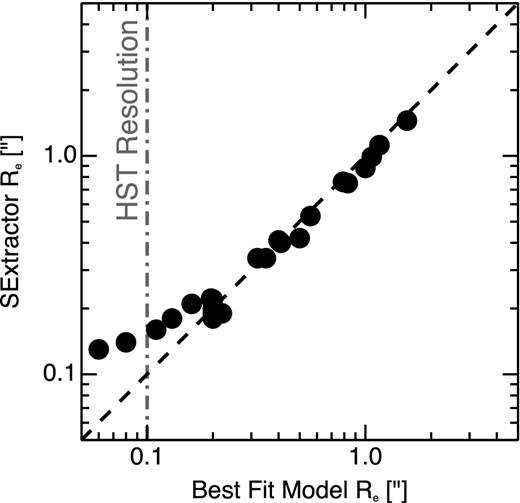
Comparison of Re determined using structural models fitted with ishape (i.e. King, Sérsic), versus those determined using SExtractor. The dashed black line is the one-to-one relation, the vertical dot–dashed line shows the resolution limit of the HST WFPC2 and ACS cameras (∼0.1 arcsec). It can be seen that for objects with Re > 3 HST resolution elements, SExtractor provides a reliable estimate of Re.
Fig. 9 shows 1 × 1 kpc thumbnails for each of our sample. It is clear from this figure the range of half-light radii displayed by our CSSs is significant. Also obvious is the fact that some of our larger (Re > 30 pc) objects show evidence for a multicomponent structure, with signs of low surface brightness outer structures that maybe provide insights into their formation mechanisms. The structural fitting analyses support this observation, with the larger objects often being poorly fit by single component models, further validating our decision to use model independent effective radii where possible. For the present paper we leave off investigating the detailed structures of our objects, relying only on the simple (usually non-parametric) estimate of Re described above which can most easily be compared to literature samples.
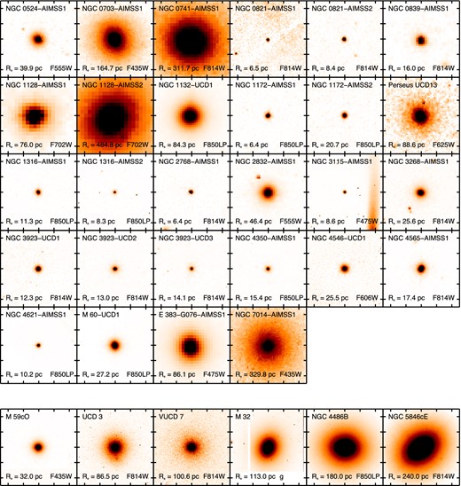
Upper panels: thumbnails of our CSS sample. Each thumbnail is 1 × 1 kpc. The measured effective radius for each CSS is provided at the bottom left of each panel, the filter of the image used to produce the thumbnail is given in the bottom right. In all cases except M 32 the imaging is from the HST, for M 32 a g-band MegaPrime image is used due to the large size of M 32 on the sky. It is clear from these images that the more extended objects (those with Re ≳ 30 pc) often appear to have additional lower surface brightness outer components. Lower panels: six literature CSSs to provide a comparison sample.
In order to allow consistent comparison of our data with the literature samples we have reestimated the sizes of the seven compact Coma cluster objects from Price et al. (2009), because the Re values given in Price et al. (2009) are provided for two component structural models separately, and not for the total light distribution, and are therefore unsuitable for comparison with other literature data. Our remeasured sizes for the Coma cluster objects are CcGV1 = 264.6 ± 36.8, CcGV9a = 344.1 ± 47.9, CcGV9b = 311.5 ± 43.3, CcGV12 = 152.3 ± 1.2, CcGV18 = 205.8 ± 28.6, CcGV19a = 208.8 ± 29.1, and CcGV19b = 99.4 ± 13.8 pc.
3.5.2 Photometry
In addition to providing size estimates for our CSSs we have also obtained new, or reanalysed existing, imaging data for each CSS. Briefly, this photometry includes the optical HST images used to select the CSSs, new SOAR/Goodman U, B, V, and R images obtained for several Southern hemisphere AIMSS CSSs, as well as reanalysed SDSS DR9 (Ahn et al. 2012) u, g, r, i, and z photometry for equatorial and Northern hemisphere objects within the SDSS footprint. Where possible we have also reanalysed archival 2MASS (Skrutskie et al. 2006), HAWK-I (Pirard et al. 2004), and NEWFIRM (Probst et al. 2004) IR images for each CSS. Where the data required reduction (i.e. the SOAR/Goodman, HAWK-I, and NEWFIRM data) we made use of standard iraf routines to carry out bias subtraction, flat fielding, and image co-addition. Zero-points for the IR data were set using 2MASS stars located within the HAWK-I and NEWFIRM fields of view. For the Goodman data we made use of standard star fields (from Landolt 2009) observed at similar airmass, immediately after the science target to provide zero-points accurate to <0.03 mag in all bands.
For all analyses, we proceeded in a similar manner to that described in Section 3.5.1. We first downloaded the calibrated frames, used iraf/ELLIPSE or a median subtraction to remove the large-scale host galaxy light, determined a curve-of-growth magnitude for the CSS, then applied a correction for foreground extinction based on Schlafly & Finkbeiner (2011). We find that the background subtraction and reanalysis is particularly vital for SDSS photometry, where the catalogued photometry frequently suffers from catastrophically under- or overestimated magnitudes and always underestimates errors for CSSs near to larger galaxies (frequently providing errors of <0.01 mag for u-band photometry of faint CSSs).
3.6 Stellar mass determination
To determine stellar mass estimates for the CSSs, both for our AIMSS discovered objects and the objects compiled into our master catalogue, we use a modified version of the stellar mass estimation code first presented in Kannappan & Gawiser (2007) and later updated in Kannappan et al. (2013). Briefly, the code fits photometry from the Johnson-Cousins, Sloan, and 2MASS systems with an extensive grid of models from Bruzual & Charlot (2003) assuming a Salpeter IMF. Each collection of input CSS photometry is fitted by a grid of two-SSP, composite old+young models with ages from 5 Myr to 13.5 Gyr and metallicities from Z = 0.008 to 0.05. This range of age and metallicity is sufficient to adequately cover those displayed by all of our CSS types, from YMCs to ancient GCs. The derived stellar mass is determined by the median and 68 per cent confidence interval of the mass likelihood distribution binned over the grid of models. Following the procedure used in Norris & Kannappan (2011), we rescale the derived stellar masses by a factor of 0.7 in order to match the ‘diet’ Salpeter IMF of Bell & de Jong (2001). We do this in order to make our stellar mass estimates more consistent with a Kroupa IMF which appears to be a better fit to observational data than Salpeter for both GCs (Strader et al. 2011a) and relatively low-mass early-type galaxies (those with σe ∼ 90 km s−1; Cappellari et al. 2013b). Therefore, as the stellar masses of our GC, UCD, and cE sample overlap with, and transition between the stellar masses of GCs and low-mass early-type galaxies, a Kroupa IMF would appear to be the most logical choice of IMF to apply.
Fig. 10 shows our derived stellar masses versus those from the literature (calculated using a range of techniques including SSP fitting and single band M/L ratios) for a sample of 46 objects in common. The agreement between the different mass estimates is remarkably good, considering the inhomogeneous nature of the input photometry, and the different approaches used to estimate stellar mass in the literature. Our stellar mass measurements are systematically lower, with ours on average being 65 per cent of the literature values, almost exactly as expected given that our stellar masses aim to be Kroupa-like, and most literature measurements are made assuming a Salpeter IMF. There is also some evidence for a tendency for our stellar masses to be even lower than expected when compared to the literature ones for M⋆ < 5 × 10⁶ M⊙. However, this only affects a handful of objects in the comparison, and at most 3 of the sample of 28 new objects presented here. The level of the divergence is also within the typical factor of 2 systematic error between different mass estimations.
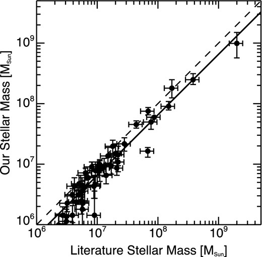
Comparison of our derived stellar masses with literature values for 46 objects in common. The error bars for our stellar masses are our errors derived using the procedure outlined in Section 3.6, while the error bars for the literature data are purely illustrative (20 per cent of measured values), as most literature analyses do not provide errors. Systematic errors are not included but are >50 per cent (e.g. Kannappan & Gawiser 2007). The dashed line is the one-to-one relation, while the solid line is the best-fitting relation for the data. Our stellar mass estimates are on average 65 per cent of the literature ones, as expected given our assumption of a Kroupa-like IMF compared to a Salpeter IMF for most literature measurements.
3.7 Classifying host galaxy environments
Until recently almost all confirmed CSSs were discovered in massive galaxy clusters, leading to the belief that the cluster environment could be responsible for forming such systems (e.g. forming UCDs by the ‘threshing’ of nucleated galaxies by cluster potentials; Bekki, Couch & Drinkwater 2001a). However, in recent years several CSSs located in field and group environments have been found (e.g. Hau et al. 2009; Norris & Kannappan 2011; Huxor et al. 2013), indicating that cluster environments are not essential for CSS formation.
We deliberately did not use environment as a selection factor in choosing CSS candidates for spectroscopic observations, in order to ensure that we did not bias our selection in favour of high-density environments. However, after observing and confirming the nature of our CSSs we then made an (admittedly crude) estimate of the environments of their host galaxies. In general to classify the environment of the CSSs we again make use of the 2MASS All Sky Redshift Survey group catalogue of Crook et al. (2007). To make a rough classification into field, group, and cluster environments we use the number of galaxies found in the same structure as the host galaxy, as found in the Crook et al. (2007) catalogue. Then using agreed classifications in the literature (i.e. that the Fornax cluster is a cluster, that NGC 3923 is in a group) we define the limits between environments as follows: field environments have 10 or fewer members, groups have more than 10 members and fewer than 40, clusters have more than 40 members.
Several AIMSS galaxies are not in the Crook et al. (2007) catalogue, so in these cases (NGC 0034, NGC 0821, NGC 1172, NGC 3115, and ESO383-G076) we base their environmental classification on literature determinations. We also reclassify NGC 4546 and the Sombrero galaxy as field galaxies, in contrast to the Crook et al. (2007) determination that these are members of the Virgo cluster, despite their lying at least 3 Mpc from the Virgo cluster centre.
While admittedly very crude, this classification does at least allow us to demonstrate that CSSs of all masses are found associated with galaxies in a wide variety of environments, from very isolated galaxies such as NGC 4546, NGC 3115, or the Sombrero, to massive galaxy clusters. This should not be a surprising finding given the existence of the prototypical cE, M32, in a small group environment.
Our classifications are also in general in reasonable agreement with a more physical classification based on group central galaxy stellar mass to halo mass ratio, which is not applicable to all our sample galaxies because of missing stellar masses for the relevant group dominating galaxies. Using this alternative approach, the stellar masses of NGC 4546, NGC 3115, and the Sombrero (all considered dominant in their local environments) – lie in the range expected for group centrals in haloes near or just above the field-to-group transition at halo mass ∼1.3 × 10¹² M⊙ where galaxy formation efficiency peaks (Leauthaud et al. 2012), but well below the group-to-cluster transition at halo mass ∼3 × 10¹³ M⊙ where cluster quenching processes take over (Robotham et al. 2006). In particular, these transitional halo mass scales correspond to central galaxy stellar masses of ∼3 × 10¹⁰ M⊙ and ∼1.3 × 10¹¹ M⊙ (e.g. Behroozi, Wechsler & Conroy 2013), while we measure stellar masses of ∼2.7 × 10¹⁰, ∼6.4 × 10¹⁰, and ∼8.2 × 10¹⁰ M⊙ for NGC 4546, NGC 3115, and the Sombrero, respectively. As all three galaxies have early-type morphology, considerable hierarchical merging has very likely occurred and may be involved in the creation of the CSSs, but physical processes specific to dense environments are less likely to be important.
4 RESULTS
Table 3 provides the measured properties of the AIMSS targets, as well as the six objects reobserved as a consistency check, and the comparison sample of seven YMCs.
Physical properties of the AIMSS objects. Distances for the host galaxies are surface brightness fluctuation distances listed in NED (http://ned.ipac.caltech.edu/) where available. Where no distances are available in the literature we assume Hubble flow distances assuming H0 = 70 km s−1 Mpc−1. Magnitude and size errors include the distance uncertainty. Because of limited photometry no reliable stellar mass estimates were possible for NGC 1172 AIMSS 1 and 2.
| Name | Distance | Re | MV | σraw | M⋆ | Environment |
|---|---|---|---|---|---|---|
| (Mpc) | (pc) | (mag) | (km s−1) | (M⊙) | ||
| AIMSS targets | ||||||
| NGC 0524-AIMSS1 | 24.0 ± 2.3 | 39.9 ± 3.8 | −12.59 ± 0.21 | 31.7 ± 3.5 | 4.96|$^{+0.00}_{-0.22}$| × 107 | G |
| NGC 0703-AIMSS1 | 82.8 ± 17.2 | 164.7 ± 28.4 | −14.97 ± 0.49 | 20.7 ± 7.2 | 3.13|$^{+1.19}_{-0.76}$| × 108 | C |
| NGC 0741-AIMSS1 | 81.3 ± 17.3 | 311.7 ± 55.0 | −17.60 ± 0.43 | 86.2 ± 4.7 | 5.96|$^{+0.28}_{-0.53}$| × 109 | G |
| NGC 0821-AIMSS1 | 22.4 ± 1.8 | 6.5 ± 0.5 | −12.08 ± 0.23 | – | 4.73|$^{+3.12}_{-1.46}$| × 106 | F |
| NGC 0821-AIMSS2 | 22.4 ± 1.8 | 8.4 ± 0.5 | −11.06 ± 0.23 | – | 7.50|$^{+0.20}_{-0.23}$| × 106 | F |
| NGC 0839-AIMSS1 | 56.0 ± 19.2 | 16.0 ± 4.1 | −12.33 ± 0.64 | – | 5.69|$^{+3.75}_{-1.75}$| × 106 | F |
| NGC 1128-AIMSS1 | 100.0 ± 16.4 | 76.0 ± 10.9 | −15.65 ± 0.47 | 63.9 ± 5.8 | 7.50|$^{+0.15}_{-0.18}$| × 108 | G |
| NGC 1128-AIMSS2 | 100.0 ± 16.4 | 484.8 ± 69.2 | −17.86 ± 0.38 | 58.1 ± 3.2 | 4.73|$^{+0.70}_{-0.80}$| × 109 | G |
| NGC 1132-UCD1 | 99.5 ± 16.9 | 84.3 ± 12.1 | −14.68 ± 0.49 | 80.1 ± 8.1 | 3.28|$^{+0.85}_{-0.90}$| × 108 | F |
| NGC 1172-AIMSS1 | 21.5 ± 2.1 | 6.4 ± 0.6 | −11.65 ± 0.22 | 40.7 ± 10.9 | 6.84|$^{+3.51}_{-2.72}$| × 106 | F |
| NGC 1172-AIMSS2 | 21.5 ± 2.1 | 20.7 ± 2.0 | −10.95 ± 0.23 | – | 1.72|$^{+1.27}_{-0.73}$| × 106 | F |
| Perseus-UCD13-AIMSS1 | 72.4 ± 7.0 | 88.6 ± 8.6 | −12.81 ± 0.22 | 35.0 ± 8.0 | 2.72|$^{+1.21}_{-1.01}$| × 107 | C |
| NGC 1316-AIMSS1 | 21.0 ± 0.7 | 11.3 ± 0.4 | −11.97 ± 0.09 | – | 4.52|$^{+4.10}_{-2.55}$| × 106 | C |
| NGC 1316-AIMSS2 | 21.0 ± 0.7 | 8.3 ± 0.3 | −10.42 ± 0.12 | – | 1.57|$^{+0.92}_{-0.67}$| × 106 | C |
| NGC 2768-AIMSS1 | 22.4 ± 2.6 | 6.4 ± 0.7 | −12.07 ± 0.24 | 38.1 ± 4.6 | 5.43|$^{+4.01}_{-2.00}$| × 106 | F |
| NGC 2832-AIMSS1 | 98.6 ± 16.7 | 46.4 ± 6.7 | −14.78 ± 0.39 | 111.3 ± 11.0 | 2.37|$^{+0.90}_{-0.81}$| × 108 | F |
| NGC 3115-AIMSS1 | 9.00 ± 0.3 | 8.6 ± 0.4 | −11.27 ± 0.12 | 36.9 ± 1.9 | 1.09|$^{+0.28}_{-0.37}$| × 107 | F |
| NGC 3268-AIMSS1 | 39.8 ± 2.8 | 25.6 ± 1.9 | −12.68 ± 0.18 | – | 3.43|$^{+1.09}_{-1.16}$| × 107 | C |
| NGC 3923-UCD1 | 21.3 ± 2.9 | 12.3 ± 0.3 | −12.43 ± 0.28 | 33.0 ± 2.1 | 1.97|$^{+0.51}_{-0.61}$| × 107 | G |
| NGC 3923-UCD2 | 21.3 ± 2.9 | 13.0 ± 0.2 | −11.93 ± 0.28 | 23.1 ± 3.6 | 6.53|$^{+2.49}_{-1.80}$| × 106 | G |
| NGC 3923-UCD3 | 21.3 ± 2.9 | 14.1 ± 0.2 | −11.29 ± 0.29 | 15.5 ± 3.6 | 2.37|$^{+1.22}_{-0.40}$| × 106 | G |
| NGC 4350-AIMSS1 | 16.5 ± 0.8 | 15.4 ± 0.1 | −12.16 ± 0.15 | 25.5 ± 9.0 | 1.57|$^{+0.60}_{-0.53}$| × 107 | C |
| NGC 4546-AIMSS1 | 13.1 ± 1.3 | 25.5 ± 1.3 | −12.94 ± 0.20 | 21.8 ± 2.5 | 3.59|$^{+0.73}_{-0.99}$| × 107 | F |
| NGC 4565-AIMSS1 | 16.2 ± 1.3 | 17.4 ± 1.4 | −12.37 ± 0.20 | 13.8 ± 8.1 | 8.19|$^{+0.42}_{-0.20}$| × 106 | C |
| NGC 4621-AIMSS1 | 14.9 ± 0.5 | 10.2 ± 0.4 | −11.85 ± 0.07 | 33.9 ± 4.4 | 1.64|$^{+0.43}_{-0.34}$| × 107 | C |
| M60-UCD1 | 16.4 ± 0.6 | 27.2 ± 1 | −14.18 ± 0.09 | 61.6 ± 1.8 | 1.80|$^{+0.18}_{-0.23}$| × 108 | C |
| ESO 383-G076-AIMSS1 | 162.8 ± 15.6 | 86.1 ± 7.6 | −15.52 ± 0.25 | – | 4.96|$^{+1.28}_{-1.20}$| × 108 | C |
| NGC 7014-AIMSS1 | 58.6 ± 4.2 | 329.8 ± 23.6 | −15.17 ± 0.16 | 20.6 ± 6.3 | 2.99|$^{+0.95}_{-1.02}$| × 108 | G |
| Reobserved objects, serendipitous observations, or objects with reanalysed photometry | ||||||
| Fornax-UCD3 | 20.0 ± 1.4 | 86.5 ± 6.2 | −13.45 ± 0.10a | 27.4 ± 5.1 | 4.96|$^{+1.28}_{-1.02}$| × 107 | C |
| NGC 2832-cE | 98.6 ± 16.7 | 375.3 ± 54.4 | −17.77 ± 0.34 | 100.5 ± 3.0 | 2.27|$^{+0.59}_{-0.47}$| × 109 | F |
| NGC 2892-AIMSS1 | 97.7 ± 16.6 | 580.9 ± 85.0 | −18.88 ± 0.37 | 137.5 ± 3.7 | 1.09|$^{+0.11}_{-0.14}$| × 1010 | F |
| NGC 3268-cE1/FS90 192 | 39.8 ± 2.8 | 299.9 ± 21.9 | −15.92 ± 0.16 | 36.8 ± 15.0 | 1.30|$^{+0.41}_{-0.11}$| × 108 | C |
| Sombrero-UCD1 | 9.00 ± 0.1 | 14.7 ± 1.4 | −12.31 ± 0.06a | 31.9 ± 2.9 | 1.64|$^{+0.43}_{-0.40}$| × 107 | F |
| M59cO | 14.9 ± 1.1 | 35.2 ± 1.2 | −13.43 ± 0.09 | 29.0 ± 2.5 | 7.49|$^{+0.11}_{-0.10}$| × 107 | C |
| ESO 383-G076-AIMSS2 | 162.8 ± 15.6 | 652.2 ± 57.5 | −17.35 ± 0.25 | 87.8 ± 8.0 | 2.60|$^{+0.53}_{-0.53}$| × 109 | C |
| YMC sample (all literature values except stellar masses) | ||||||
| NGC 0034-S&S1 | 85.1 ± 17.2 | 39.0 ± 7.8b | −15.36 ± 0.40 | – | 3.13|$^{+4.73}_{-1.94}$| × 107 | F |
| NGC 0034-S&S2 | 85.1 ± 17.2 | 31.9 ± 6.4b | −14.70 ± 0.40 | – | 2.37|$^{+2.82}_{-1.47}$| × 107 | F |
| NGC 1316-G114 | 21.0 ± 0.7 | 42.1 ± 2.6 | −12.81 ± 0.12 | 42.1 ± 2.8 | 2.72|$^{+0.71}_{-1.09}$| × 107 | C |
| NGC 7252-W3 | 67.3 ± 17.4 | 17.7 ± 4.4c | −16.30 ± 0.51 | 45.5 ± 5.2 | 1.25|$^{+1.74}_{-0.89}$| × 108 | F |
| NGC 7252-W6 | 67.3 ± 17.4 | 5.1 ± 1.3c | −14.50 ± 0.51 | – | 2.37|$^{+2.36}_{-1.47}$| × 107 | F |
| NGC 7252-W26 | 67.3 ± 17.4 | 11.9 ± 3.0c | −13.75 ± 0.51 | – | 1.37|$^{+1.24}_{-0.82}$| × 107 | F |
| NGC 7252-W30 | 67.3 ± 17.4 | 8.3 ± 2.1c | −14.68 ± 0.51 | 27.5 ± 2.5 | 2.72|$^{+2.71}_{-1.74}$| × 107 | F |
aErrors calculated by assuming photometric uncertainty of 0.05 mag combined with the measured distance uncertainty.
bSizes from Schweizer & Seitzer (2007) with errors computed assuming 0.4 mag distance modulus uncertainty to NGC 34.
cSizes from Bastian et al. (2013) with errors computed assuming 0.5 mag distance modulus uncertainty to NGC 7252.
4.1 Luminosity–effective radius
Fig. 11 shows the location of the AIMSS sample (blue stars) in size–luminosity space relative to other stellar systems, including GCs and previously known UCDs (red dots), galaxy nuclei (orange squares), YMCs (blue triangles), cEs (green open stars), dSphs (grey filled squares), dEs and dS0s (grey filled triangles), elliptical galaxies (filled black dots), Es and S0s from the ATLAS3D (grey dots), and the prototypical cE M32 indicated with a symbol of its own.
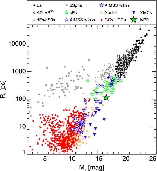
Effective radius Re versus absolute V-band magnitude MV for dynamically hot stellar systems from our master compilation. Blue stars are our observations and are filled where we have successfully measured the velocity dispersion of the object. M32 is indicated by its own symbol and labelled. It is clear that the group of six (including one literature Coma cE) non-YMC objects with MV < −14 and Re < 100 pc lie offset significantly from the more massive previously known UCDs such as Virgo-UCD7 and Fornax-UCD3, which are smaller than M32.
From Fig. 11 it is clear that most AIMSS objects occupy the previously defined region of parameter space for UCDs and cEs. However, of immediate interest is the presence of a population of six objects (five AIMSS objects plus one previously known Coma cluster cE) that are considerably brighter at fixed size than previously known UCDs (with ∼ 30 < Re [pc] ≲ 100, and MV < −14.0). The smallest of these six objects (M60-UCD1, MV ∼ −14, Re ∼30 pc) has been previously described in Strader et al. (2013) as the ‘Densest Galaxy’. Our newly discovered objects indicate M60-UCD1 is the first of a population of unusually compact and luminous (even for UCDs) stellar systems. The six objects lie within a region to the right (i.e. more luminous) side of the usual UCD trend that had previously only been inhabited by much younger and hence more luminous YMCs (see Section 4.2) and by the nuclei of galaxies. The new objects also appear to extend the apparent hard limit on the bright side of the elliptical galaxy size–luminosity trend all the way down to the star cluster mass regime.
These new objects are found in all environments, with two found in the field (NGC 1132-UCD1 and NGC 2832-AIMSS1), one found in a group (NGC 1128), and three found in clusters (CcGV19b, NGC 4649-AIMSS1, ESO383-G076-AIMSS1). This diversity should not be too surprising as M32 itself is found in a low-N, field-like group, proving that cluster environments are not essential for forming the densest stellar systems.
Another observation to be made from Fig. 11 is the apparent rarity of CSSs more luminous than MV = −13. This observation is examined in more detail in Fig. 12, where all known massive GCs, UCDs, and cEs with –10 < MV < −18 and Re < 400 pc are plotted. The top panel of this figure shows the histogram of the magnitudes of these objects, with a dashed horizontal line denoting the median number of objects per bin with MV < −13. There appears to be a roughly constant number of objects brighter than MV = −13, but fainter than this value, the number of objects increases dramatically. Of course the sample being examined here is in no way homogeneous, having been built from many disparate surveys, and is therefore not a well-defined statistically complete sample. However, it is also clear that brighter objects at fixed size are observationally simpler to find, so the observed drop-off in CSS frequency fainter than MV < −13 is not likely to be due to simple selection effects in the surveys used to build the sample. In fact many of the input literature samples were specifically designed to spectroscopically observe all objects irrespective of size brighter than magnitude limits of around MV ∼ −15.5 (e.g. Jones et al. 2006), further indicating that the observed drop off is likely real. It is also interesting that MV > −13 is exactly the upper limit for objects formed in star cluster like processes suggested by Norris & Kannappan (2011) on the basis of statistical arguments about the GC luminosity function, as first suggested by Hilker (2009).
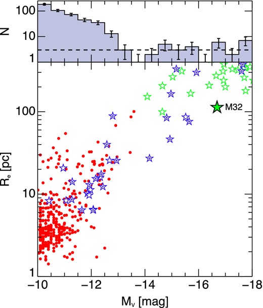
Lower panel: effective radius versus absolute V-band magnitude for all known massive GCs, UCDs, and cEs with −10 < MV < −18 and Re < 400 pc. Upper panel: histogram of the MV values of the selected objects, with the statistical 1σ uncertainties shown by the error bars. The dashed line shows the median number of objects (three) per bin for MV < −13. It is clear that there is a drop off in the number of objects for MV < −13.
4.2 Stellar mass–effective radius
Returning to the question of the six unusually bright objects in the MV–Re parameter space, one explanation for their location is that, like YMCs, these objects are younger, and hence brighter than the generally old UCD population at the same stellar mass. This possibility is a valid concern as some cEs are observed to have intermediate stellar ages (e.g. Schiavon, Caldwell & Rose 2004; Chilingarian et al. 2009; Huxor et al. 2011b; Miner, Rose & Cecil 2011), although this may be due to a ‘frosting’ of recent star formation and not a dominant mass component. As we currently lack suitable spectroscopic estimates of age for many of our objects we therefore turn to the stellar mass estimates to address this question.
Fig. 13 convincingly demonstrates that age differences are not responsible for the observed offsets. In the stellar mass–Re plane the gap between the six unusual objects and the main UCD track (as defined by the dashed-line fit to bright ellipticals, compact ellipticals, bulges and UCDs from Dabringhausen et al. 2008) is decreased, but five of the six remain to the right of the main UCD track. The behaviour of the YMCs in this plane is also instructive, as these truly young clusters, which in the MV–Re plane all lie far to the right of the main UCD trend, are now mostly consistent with the general trend, indicating that they were offset due to their youthful luminosity.
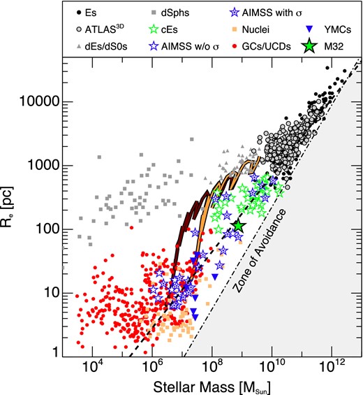
Effective radius Re versus stellar mass for CSSs and comparison samples. Symbols are the same as those defined in Fig. 11. The dot–dashed line is the by-eye fit to the edge of the elliptical galaxies, cEs and dE nuclei, as determined by Misgeld & Hilker (2011), having the form Reff(M) > 2.24 × 10⁻⁶ M|$_{\star }^{4/5}$| pc M|$_{\odot }^{4/5}$|. The orange and brown solid lines show the simulated evolution of two nucleated dEs as they are stripped by the potential of a larger galaxy from Pfeffer & Baumgardt (2013, their simulations 3 and 17). The dashed line is the fit to bright ellipticals, compact ellipticals, bulges, and UCDs from Dabringhausen et al. (2008). In this plot, the separation between the unusually dense objects (mostly to the right of the dashed line) and the previously known UCDs (near and to the left of the dashed line) is even more clearly demonstrated.
The location of the unusually bright objects also demonstrates that three of the objects (NGC 1128-AIMSS1, NGC 1132-UCD1, ESO383-G076-AIMSS1) are amongst the best analogues in terms of mass and size for M32 yet found.
We overplot in Fig. 13 the evolutionary tracks (solid orange and brown lines) of two nucleated dE galaxies as they are tidally stripped from the simulations of Pfeffer & Baumgardt (2013). The simulations are numbers 3 (brown) and 17 (orange) from Pfeffer & Baumgardt (2013). They are both of dE, N galaxies on elliptic orbits with apocentre of 50 kpc and pericentre of 10 kpc around a cluster centre which has properties chosen to match M87 in the Virgo cluster. Simulation 3 originally has a nucleus with Re = 4 pc and MV = −10, simulation 17 initially has a nucleus with Re = 10 pc and MV = −12. Both are simulated for a total of 4.2 Gyr. We use these simulations to stand in for simulations of any nucleated dwarf galaxies undergoing stripping, as at present very few simulations of the stripping of later type dwarfs have been carried out, but we expect that the stripping of other dwarf galaxy types should produce reasonably similar results. The simulations of Pfeffer & Baumgardt (2013) demonstrate that the remnants of the stripping of dE, Ns can resemble almost all massive GCs and UCDs, even the most extended (Re ∼ 100 pc) and massive (M ∼ 108 M⊙) UCDs such as Fornax-UCD3, Virgo-UCD7, and Perseus-UCD13. However, it is also clear that these simulations cannot reproduce the properties of the unusually massive compact objects. To produce such objects by stripping requires the objects being stripped to be significantly more massive initially, making their likely progenitors true ellipticals, S0s, or bulged spiral galaxies.
A further interesting observation in Fig. 13 is that despite the very high density of some of the new AIMSS objects, none of them (and no objects at all) have significantly violated the dot–dashed line into the region called the ‘zone of avoidance’ by Misgeld & Hilker (2011). This region to the right of the dot–dashed line is the equivalent of the ‘zone of exclusion’ that Burstein et al. (1997) found to exist for early-type galaxies. It therefore appears that there is a universal relation limiting the maximum stellar density an old dynamically hot stellar system may have, although this is not as simple as the limit being a constant mass surface density limit (see Section 4.3). The existence of such a universal relation would be extremely interesting, especially considering the huge differences in composition and structure between apparently dark matter free GCs and dark matter dominated giant ellipticals. We discuss this topic in more detail in Section 5.3.
In contrast to the further support for the existence of a ‘zone of avoidance’, the new AIMSS objects, along with other less massive but large GC-like objects (e.g. Brodie et al. 2011; Forbes et al. 2013), and fainter cEs continue to weaken evidence for a suggested mass–size relation (see e.g. Dabringhausen et al. 2008; Murray 2009; Norris & Kannappan 2011) for CSSs. It is now clear that CSSs can display a range in mass which varies by more than a factor of 100, at fixed size. This is more than a factor of 10 times the range seen for massive early types. Observationally difficult to find fainter stellar systems with large radii are gradually being discovered and these fill in the space between classical GCs and dSphs. It seems possible that given time this region will be completely filled, further blurring the distinction between star clusters and galaxies.
One final observation is that there are hints of a dichotomy in the cE population, between objects that appear to be a continuation of the elliptical galaxy population (the block centred at around 400 pc and 5 × 10⁹ M⊙), and a population possibly associated with dwarf galaxies (the tail dropping down from around 300 pc and 2 × 10⁸ M⊙), we investigate this point further in Section 4.3.
4.3 Stellar mass–mass surface density
Fig. 14 shows the location of the various stellar systems in the stellar mass–effective mass surface density (half the stellar mass divided by the area within the half-light radius) plane. This space is a mass versus average surface brightness plot, where the age dependence of the surface brightness is removed.
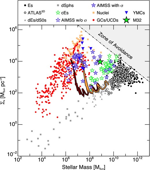
Stellar mass versus effective stellar mass surface density for dynamically hot stellar systems. Symbols are the same as those defined in Fig. 11. The effective stellar mass surface density is calculated as Σe = M⋆ / 2πR|$^2_{\rm e}$|. The ‘zone of avoidance’ translated from that shown in Fig. 13 is shown by the grey shaded region. The solid orange and brown lines are the same simulations from Pfeffer & Baumgardt (2013) as shown in Fig. 13. In this plane, it is even clearer that there is a separation between the densest objects discussed here and the majority of the CSS population.
It is clear from this plot that several of our new AIMSS objects (including M60-UCD1; Strader et al. 2013) lie in a region of parameter space where previously only M32, or the most massive galaxy nuclei (or bulges), were known to exist. It is also of note that the simulated stripped dE, Ns from Pfeffer & Baumgardt (2013) also cannot reproduce the location of these dense stellar systems in the stellar mass – effective mass surface density plane, again indicating a likely origin for most of these objects in more massive non-dwarf galaxies, if they are indeed the result of stripping. In fact, of this group only M60-UCD1 has properties that could be explained as being the result of the stripping of a dwarf galaxy (albeit on the massive end of the dwarf population), whereas all the rest must have resulted from the stripping of giant galaxies.
It is also immediately obvious in Fig. 14 that several AIMSS objects, and literature cEs, lie in a region of parameter space much closer to dwarf galaxies than to classical ellipticals, although the majority of cEs found to date are closer to classical Es (with a division at ∼7 × 10⁸ M⊙). This observation may reflect a dichotomy in galaxy stripping. In a stripping scenario of UCD or cE formation, the stripping process simply removes the outer parts of galaxies to reveal the bound stellar structure within the galaxy, be it a nucleus, or for larger cEs potentially an entire galaxy bulge. Therefore, the process should work for any galaxy with a central bound structure like dEs/dS0s, Es/S0s, or spirals, but not most dSph galaxies. This picture implies two types of resulting stripped object, one from the stripping of nucleated dwarfs and another form the stripping of bulged massive galaxies. It is also possible that some cEs are the result of dissipative merging like classical ellipticals (see e.g. Kormendy & Bender 2012).
In the stripping scenario a galaxy can move towards the upper left of Fig. 14, as the tightly bound stellar structure at the centre of the galaxy comes to dominate more and more of the total remaining galaxy. Therefore, a dwarf with a central nuclear star cluster similar to those in the plot will move away from the dwarf sequence towards the UCD region, as it is being stripped. This is precisely what the simulations by Pfeffer & Baumgardt (2013) clearly show; that a dE, N when stripped will gradually evolve downward in the luminosity–size plot from the dwarf space, through the region inhabited by large UCDs (such as Fornax-UCD3 and Virgo-VUCD7), possibly even reaching sizes and luminosities indistinguishable from GCs.
Fig. 14 also demonstrates that the densest old stellar systems found in the Universe are galaxy nuclei. Our comparison sample of YMCs do reach similar densities, but after 10 Gyr of dynamical evolution and stellar mass loss their structures are likely to change dramatically.
4.4 Stellar mass–velocity dispersion
Fig. 15 shows the location of the various stellar systems in the stellar mass versus velocity dispersion (σ) plane. It is clear from this figure that in agreement with Forbes et al. (2008, their fig. 5) we find that there is a distinct separation between early-type galaxies and star clusters, with transitional objects such as massive UCDs and cEs bridging the gap between the two sequences at the high-σ end, and dSphs bridging the gap at the low-σ end. In the region between 10 and 70 km s−1 there is a clear splitting of the plot into two tracks. In particular, it is clear that the massive ellipticals display one slope, with a break at a central σ of around 105 km s−1, followed by lower mass Es, S0s, dwarfs (dEs and dS0s on the plot) displaying a steeper slope which is closer to that of the GCs. However, the dEs/dS0s and more massive dSphs are offset from the GCs/UCDs towards higher masses, by a maximum factor of around 100 at 30 km s−1. This offset is in good agreement with the MK ∼ 5 offset between the two sequences determined by Forbes et al. (2008).
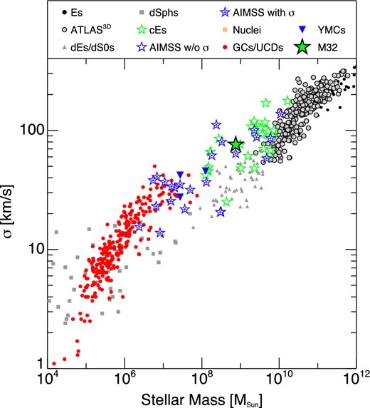
Stellar mass versus velocity dispersion for our various stellar systems. There is an obvious bifurcation between the star clusters on one side, galaxies on the other, and CSSs on both loci. In this space, tidal stripping tends to move objects towards the left-hand (lower mass) side of the plot at roughly constant velocity dispersion (Bender et al. 1992; Chilingarian et al. 2009). Therefore, most cEs and massive UCDs are consistent with being stripped from objects originally 10–100 times larger than their current mass (mostly lower mass Es/S0s and more massive dEs). However, a possible second group of objects (with the most extreme examples being two AIMSS objects and one literature cE with σ ∼ 20 km s−1) with properties more like those of normal dEs also seem to exist, with these objects perhaps being less severely stripped nucleated dwarf galaxies.
Also of interest in Fig. 15 is the location of the cE population. The majority of the cEs lie offset to the left (lower mass) from the main galaxy trend, exactly as expected for objects that have been stripped down from initially larger normal galaxies. The magnitude of the offset (assuming central velocity dispersion is unaffected by the stripping process as claimed by Bender et al. 1992; Chilingarian et al. 2009) suggests that the cEs have lost up to 99 per cent of their original mass. There is also evidence in this plot for the dichotomy we suggest exists in the cE population, with several of the AIMSS and literature cEs having velocity dispersions similar to those of massive dwarfs (∼40–50 km s−1), while the bulk of the cE population has velocity dispersions more consistent with the elliptical sequence (∼100 km s−1).
5 DISCUSSION
5.1 Compact stellar system formation
In the last few years it has become generally accepted that the UCD population is composite (e.g. Brodie et al. 2011; Chiboucas et al. 2011; Chilingarian et al. 2011; Da Rocha et al. 2011; Norris & Kannappan 2011; Strader et al. 2011b; Mieske et al. 2013), with both UCDs arising in star formation events (which also produce ‘normal’ star clusters such as GCs) as well as a population of objects resulting from the tidal stripping of galaxies. One piece of evidence for this duality comes from the normally close correspondence between the frequency and luminosity of UCDs and the total number of GCs in the host galaxy GC population (Hilker 2009; Norris & Kannappan 2011; Mieske, Hilker & Misgeld 2012), combined with the observation that outliers exist which cannot be adequately explained by extrapolation of the GCLF (Norris & Kannappan 2011).
It is also the case that several of these objects, which cannot be explained by an extrapolation of the GCLF, have properties indicative of a stripped origin. For example, the UCD of NGC 4546 is found to be young (∼3 Gyr) while its host galaxy is uniformly old (∼10 Gyr). In addition, this UCD was found to counter rotate around the host galaxy, which is a ‘smoking gun’ of an accretion event. Penny et al. (2014) also find that UCD13 in the Perseus cluster is likely to be the result of the stripping of a nucleated dwarf galaxy by NGC 1275, based on the UCD's colour, size, metallicity, velocity dispersion, dynamical mass, and proximity to NGC 1275.
A further piece of evidence for the duality of UCD types comes from the observed kinematics of UCDs around M87. Strader et al. (2011b) found that the position–velocity patterns of the UCDs near to M87 showed signatures of both radial and tangential orbits, as would be expected from stripped galaxies and surviving extended star clusters, respectively.
As already discussed, the simulations of Pfeffer & Baumgardt (2013) clearly show that objects resembling Perseus-UCD13, Virgo-UCD7, Fornax-UCD3 and NGC 4546-UCD1 can be produced by the stripping of nucleated dwarf galaxies, with the largest UCDs (∼Re = 50–100 pc) being created when some of the stellar envelope of the dwarf is retained. However, the stripping of dwarf galaxies cannot explain the production of the new M32-like objects we present here, as the total stellar masses of dwarfs themselves are roughly the same as the final structures we seek to explain (∼108–109 M⊙), while dE/dS0 radii are a factor of 10 too large. Therefore, to create these new M32-like objects we must assume that either they are created by the stripping of bulges from spiral or early-type galaxies as suggested by e.g. Faber (1973), Bekki et al. (2001b), Chilingarian et al. (2009), Graham (2013) and observed to occur in certain cases (e.g. Forbes et al. 2003; Smith Castelli et al. 2008; Huxor et al. 2011b), or that these objects are merely the low-luminosity extension of the true elliptical sequence (e.g. Kormendy & Bender 2012; Graham 2013), or some combination of the two scenarios. We note that Chilingarian et al. (2009) included some simulations of a tidally stripped barred spiral galaxy in a Virgo cluster-like potential. They found that stripping leads to a strong increase in surface brightness (see their fig. 1) similar to that predicted by Pfeffer & Baumgardt (2013) for stripping of dE, N galaxies. They also confirmed the conclusion of Bender et al. (1992) that tidal stripping moves objects to a lower stellar mass whilst leaving the velocity dispersion largely unchanged.
An additional observation about the M32-like objects is that they are found in a range of environments which are very different to the Local Group where M32 is located. One is located near an isolated elliptical, another is in a group, and the last is in a dense cluster, further indicating the universal nature of the formation mechanism for this type of object. These new objects therefore carry the apparently paradoxical message that although they are rare, they are also ubiquitous, perhaps indicating that they are commonly created but short lived.
Having now determined that at least two types of process can create CSSs, star formation related and galaxy interaction related, it remains to determine which objects were formed by which process. The close connection between UCD luminosity and GC system size, combined with the known properties of the GCLFs of galaxies, led Norris & Kannappan (2011) to suggest MV ∼ −13 (M⋆ ∼ 7 ×10⁷ M⊙) as the upper limit of ‘star cluster’ type UCD formation. Above this mass limit all objects would be stripped nuclei or bulges, and below the limit a combination of both types would exist, with star cluster type UCDs increasingly dominating to lower masses. The suggested upper mass limit is close to the dividing mass found by Mieske et al. (2013) (M⋆ > 107 M⊙), above which all UCDs were found to have enhanced M/L, indicative of either the presence of a dark mass (in this case massive black holes as the baryonic densities are too high for dark matter to significantly affect the M/L) or an IMF change, and below which UCDs display bimodal M/L, some being consistent with normal stellar populations and no dark mass. This mass is also in the middle of the range suggested by Chilingarian et al. (2011) who found that above 108 M⊙, tidally threshed objects were dominant, while below 107 M⊙ objects associated with red (metal-rich) GC formation were the norm.
To these previous findings we add the observation from Fig. 12 that the number of CSSs (with Re < 400 pc) appears to drop notably, to an almost constant value above MV ∼ −13. As previously discussed, although this finding relies on a heterogeneous data set, it is also the case that the brighter objects should be easier to find, so we doubt that any simple selection effect can be affecting all previous studies to create this feature.
Taking these observations together, it is possible to sketch out a rough outline of where the different stellar systems lie in the mass–size plane (Fig. 16). The red ellipses show the regions inhabited by ellipticals, early-type dwarfs, and dSphs; and the blue region shows where star cluster type objects can be found, including their upper mass limit at ∼7 × 10⁷ M⊙. It should be noted that even star clusters may themselves have multiple distinct origins (e.g. Elmegreen 2008; Pfalzner 2009; Baumgardt et al. 2010), although this would not affect our conclusions about the formation of other stellar systems. The green region indicates where the stripped remains of galaxies are expected to be found, based on known objects which are strongly suspected to be stripped: several cEs and M 32, the brightest known literature UCDs, Perseus-UCD13 and NGC 4546-UCD1, and the known locations of dwarf nuclei. The yellow arrows are illustrative tracks for objects being stripped, with the left-hand track for nucleated dwarf galaxies and the right for bulged massive galaxies. It is also possible that some fraction of the more massive objects (cEs in general) are a low-mass extension of the classical elliptical sequence as suggested by Kormendy & Bender (2012).
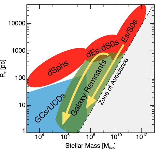
Idealized version of Fig. 13 showing the location of different CSSs and galaxy reference samples in the mass–size plane. The red ellipses show the location of the various early-type galaxy sequences, and the blue wedge shows the location of star cluster type systems (i.e. GCs and UCDs) including their upper mass limit at around 7 × 10⁷ M⊙. The green region shows the location of objects formed through the stripping of larger galaxies, which have previously been called cEs (if stripped bulges) or UCDs (if stripped dwarf galaxy nuclei) but are really members of the same sequence of objects. The yellow arrows show idealized evolutionary tracks for galaxies being stripped, with the left-hand track being nucleated dwarfs undergoing stripping, the right-hand track is for bulged Es, S0s, and spirals. Additionally, some cEs could also represent the extension of the classical E sequence to low mass.
5.2 Predictions for other compact stellar system properties
In this paper, we have described the luminosity, size, stellar mass, and velocity dispersion behaviour of CSSs. Given the conceptual framework for CSS formation suggested in Fig. 16 we can make several predictions for other CSS properties.
The first prediction is that star clusters versus stripped (or giant elliptical sequence extension) CSS properties should display bimodality. For example, stripped nuclei or bulges are expected to display multicomponent surface brightness profiles, due to the lingering presence of remnants of the outer galaxy structures (see e.g. Pfeffer & Baumgardt 2013). In contrast, massive star clusters are likely to retain the simple structures of their lower mass counterparts. Additionally the orbital properties of CSSs formed by each route are likely to be different. As discussed in Strader et al. (2011b) CSSs formed by the stripping of nuclei and bulges are expected to have preferentially radial orbits, as they are formed by stripping during close passages of the more massive galaxy. Conversely, because of survivor bias, massive star clusters should be preferentially on tangential orbits as these avoid close passages of the galaxy centre.
A further prediction is that CSSs formed through stripping should contain intermediate-mass/supermassive black holes with masses appropriate for the original mass of the galaxy before it was stripped. This should in general mean that they are overmassive relative to the standard MBH-M⋆ relation. In contrast star cluster type CSSs should either have no massive black holes or at most ones that follow the standard MBH-M⋆ relation. Work by Mieske et al. (2013) has already demonstrated that this seems to be the case; they find that massive CSSs have significant amounts of dark mass consistent with overmassive central black holes, while lower mass CSSs hint at a bimodal distribution of dark mass with some consistent with no dark mass (presumably star cluster type CSSs) and some consistent with significant dark mass (presumably stripped objects).
CSSs are also expected to differ in their stellar populations. The majority of the GC populations of galaxies are ancient (with age ∼10 Gyr), whereas stripped nuclei and bulges can potentially display a range of ages, especially in the field, where actively star-forming galaxies can be stripped. Therefore, spectroscopically determined ages are a potentially powerful way to separate star clusters from stripped nuclei in the CSS population. There are also likely to be environmental dependences of the CSS stellar populations, in the sense that in lower density environments the galaxies being stripped are more likely to be later type and hence younger than the objects being stripped in denser environments (primarily dEs and dS0s), leading to the prediction that field/group stripped objects should on average be younger than cluster stripped CSSs.
Metallicities of stripped nuclei and bulges should be significantly higher than expected for their current masses, if they were really merely an extension of the early-type galaxy population. This is because early-type galaxies display a mass–metallicity relation, in the sense that more massive galaxies are more metal rich (up to a point), while stripping reduces mass without affecting the central metallicity of the stellar population (Chilingarian et al. 2009). Recent work (by e.g. Chilingarian et al. 2009; Francis et al. 2012) already demonstrates that massive cEs including M32 and NGC4486B have metallicities consistent with those of much larger galaxies, rather than with the observed mass–metallicity relation for early types. In fact M32 is offset from the normal mass–metallicity relation by more than 0.6 dex in metallicity (or alternatively by more than 4 mag in luminosity). In the case where there is an additional population of true low-mass classical ellipticals the predictions would be generally the same as those for the stripped nuclei with the possible exception of the metallicities. The metallicities of low-mass classical ellipticals could follow the general mass–metallicity trend, alternatively, the high density of the objects (leading to a higher potential) could lead to higher levels of enrichment than less compact early types of the same mass due to the increased retention of supernova ejecta.
5.3 The zone of avoidance
Fig. 14 shows an apparent mass dependence of the maximum of the effective surface mass density varying from ∼106 M⊙ pc−2 for galaxy nuclei, to ∼103 M⊙ pc−2 for the most massive ellipticals. However, Hopkins et al. (2010) demonstrate that in fact nuclei, the MW nuclear disc, Cen A GCs, UCDs, and ellipticals all reach the same maximum surface mass density Σmax of ∼105 M⊙ pc−2. The apparent mass trend in effective surface mass density Σeff is simply the result of the evolutionary change in the structures of the objects leading to the effective radius being larger, and the effect of the central structure being diluted. In the simplest example the Σmax of a nucleated dwarf clearly must be roughly the same as that of a pure nucleus, but the Σeff will be considerably lower, because the exponential component of the dwarf has a lower mass surface density and extends the effective radius of the structure considerably. Hopkins et al. (2010) also noted that the maximum surface mass density is reached over a considerable range of scales for the different objects, indicating that it is not simply a limit on the three-dimensional stellar density.
Hopkins et al. (2010) ascribed the observation of a constant Σmax for nuclei, UCDs, and ellipticals to feedback from massive stars in the baryon-dominated cores of star clusters and galaxies. One potential problem with this picture is that galaxy nuclei do not appear to form in single formation events (see e.g. Walcher et al. 2006; Seth et al. 2010), and if they are gradually built up over time in a series of smaller formation events, this feedback is likely to prove less effective as the radiation field from young massive stars in each star formation event is smaller than would be present if all of the mass was produced simultaneously.
Nevertheless, although we have searched for objects that breach the observed effective surface mass density limit we have not yet found any culprits. It therefore appears that at least one physical process is responsible for limiting the Σmax and through a conspiracy with the structural changes of these various object types this leads to a well-defined ‘zone of avoidance’. Whatever this physical process is, it is responsible for limiting Σmax for a diverse group of objects that had a wide range of formation processes: from formation in a one-off near instantaneous burst (the GCs), through repeated smaller star formation events (the nuclei), up to building up through hierarchical merging over Gyr time-scales (the ellipticals).
6 CONCLUSIONS
We have presented the first results from the AIMSS survey. By examining the luminosities, masses, effective radii and velocity dispersions of a sample of newly discovered CSSs, along with literature compilations, we have reached the following conclusions.
We have discovered several new stellar systems which completely bridge the gap between star clusters and galaxies in the mass–size, mass–mass surface density, and mass–velocity dispersion planes.
Three of our newly discovered CSSs (NGC 1128-AIMSS1, NGC 1132-UCD1, ESO 383-G076-AIMSS1) are the closest known M32 analogues found to date. These objects are significantly more massive than typical UCDs of similar radius. When combined with three other unusually dense stellar systems and M32, their environmental distribution shows that these objects can be formed in all galactic environments from the field to galaxy clusters. The relative rarity of these objects, combined with their environmental ubiquity, might point to them being formed often but being short lived when they do arise.
The existence of our CSSs, along with other recently discovered objects, throws into doubt a universal well-defined mass–size relation for CSSs. These objects do however, further support the existence of a universal ‘zone of avoidance’ for all dynamically hot stellar systems, beyond which no isolated system can add stellar mass at fixed size.
By examining the luminosity distribution of CSSs, we offer further support for the idea that MV ∼ −13 (M⋆ ∼ 7 × 10⁷ M⊙) is a fundamental limit for the creation of CSSs in star cluster formation processes. At larger masses all objects, whether called UCDs or cEs, are likely created by the tidal stripping of larger galaxies, though we cannot rule out dissipative merging in some cases. Below this mass a combination of star clusters and stripped nuclei exist, with the fraction of star clusters increasing towards lower mass.
We suggest that two types of UCD/cE-like object exist, one type being the result of the tidal stripping of galaxies with bulges (Es, S0s, and spirals), and the other the result of the stripping of nucleated dwarfs (dEs/dS0s).
Finally, the fact that our CSSs are found associated with galaxies located in a range of environments from the field/loose groups to the densest clusters indicates that while dense environments may aid CSS formation (especially for the most massive CSSs which come from larger galaxies), they are not essential.
We would like to thank Joel Pfeffer for providing the output of several of his dE, N stripping simulations. We would also like to thank Remco van den Bosch and Eva Schinnerer for helpful discussions and comments, as well as Bart Dunlap and Brad Barlow for carrying out some of the observations this paper is based upon.
Support for Programme number HST-AR-12147.01-A was provided by NASA through a grant from the Space Telescope Science Institute, which is operated by the Association of Universities for Research in Astronomy, Incorporated, under NASA contract NAS5-26555.
DAF thanks the ARC for financial support via DP130100388. This work was supported by National Science Foundation grant AST-1109878.
SJP acknowledges the support of an Australian Research Council Super Science Postdoctoral Fellowship grant FS110200047.
FRF and AS-C acknowledge financial support from Consejo Nacional de Investigaciones Científicas y Técnicas, Agencia Nacional de Promoción Científica y Tecnológica (PICT 2010-0410), and Universidad Nacional de La Plata (Argentina).
Based on observations obtained at the Southern Astrophysical Research (SOAR) telescope, which is a joint project of the Ministério da Ciência, Tecnologia, e Inovação (MCTI) da República Federativa do Brasil, the US National Optical Astronomy Observatory (NOAO), the University of North Carolina at Chapel Hill (UNC), and Michigan State University (MSU).
Some of the observations reported in this paper were obtained with the Southern African Large Telescope (SALT).
Some of the data presented herein were obtained at the W. M. Keck Observatory, which is operated as a scientific partnership among the California Institute of Technology, the University of California and the National Aeronautics and Space Administration. The Observatory was made possible by the generous financial support of the W. M. Keck Foundation.
The authors wish to recognize and acknowledge the very significant cultural role and reverence that the summit of Mauna Kea has always had within the indigenous Hawaiian community. We are most fortunate to have the opportunity to conduct observations from this mountain.
This paper makes use of data obtained as part of Gemini Observatory programmes GS-2004A-Q-9 and GS-2011A-Q-13.
Based on observations obtained at the Gemini Observatory, which is operated by the Association of Universities for Research in Astronomy, Inc., under a cooperative agreement with the NSF on behalf of the Gemini partnership: the National Science Foundation (USA), the National Research Council (Canada), CONICYT (Chile), the Australian Research Council (Australia), Ministério da Ciência, Tecnologia e Inovação (Brazil) and Ministerio de Ciencia, Tecnología e Innovación Productiva (Argentina).
Based on observations made with the Isaac Newton Telescope (INT) operated on the island of La Palma by the Isaac Newton Group (ING) in the Spanish Observatorio del Roque de los Muchachos of the Instituto de Astrofisica de Canarias (IAC).
This research has made use of the NASA/IPAC Extragalactic Database (NED) which is operated by the Jet Propulsion Laboratory, California Institute of Technology, under contract with the National Aeronautics and Space Administration.
Based on observations obtained at the Southern Astrophysical Research (SOAR) telescope, which is a joint project of the Ministério da Ciência, Tecnologia, e Inovação (MCTI) da República Federativa do Brasil, the US National Optical Astronomy Observatory (NOAO), the University of North Carolina at Chapel Hill (UNC), and Michigan State University (MSU).
Based on observations made with the Southern African Large Telescope (SALT).
Some of the data presented herein were obtained at the W. M. Keck Observatory, which is operated as a scientific partnership among the California Institute of Technology, the University of California and the National Aeronautics and Space Administration. The Observatory was made possible by the generous financial support of the W. M. Keck Foundation.
Based on observations made with the Isaac Newton Telescope (INT) operated on the island of La Palma by the Isaac Newton Group in the Spanish Observatorio del Roque de los Muchachos of the Instituto de Astrofisica de Canarias.
Based on observations obtained at the Gemini Observatory, which is operated by the Association of Universities for Research in Astronomy, Inc., under a cooperative agreement with the NSF on behalf of the Gemini partnership: the National Science Foundation (USA), the National Research Council (Canada), CONICYT (Chile), the Australian Research Council (Australia), Ministério da Ciência, Tecnologia e Inovação (Brazil) and Ministerio de Ciencia, Tecnología e Innovación Productiva (Argentina).
REFERENCES
APPENDIX A: CATALOGUE
In Table A1, we provide the complete catalogue of CSSs and comparison samples described in Section 2.2. The literature sample is constructed from the following sources.
Catalogue of CSSs and comparison samples. The first three objects in the catalogue are shown to demonstrate the form of the catalogue, all objects are available in the electronic version of this table. The columns are name, type, RA, Dec., absolute V-band magnitude, stellar mass, effective radius, σ, and literature reference for catalogue objects. The type codes refer to the object types as follows: (1) Es/S0s, (2) dEs/dS0s, (3) dSphs, (4) nuclear star clusters, (5) literature GCs, UCDs, cEs, (6) AIMSS GCs, UCDs, cEs, (7) YMCs. Stellar masses are from the literature sources listed except for types 2, 5, 6, and 7 where the stellar masses were computed following the approach outlined in Section 3.6.
| Name | Type | RA | Dec. | MV | M⋆ | Re | σ | References |
|---|---|---|---|---|---|---|---|---|
| (J2000) | (J2000) | (mag) | (M⊙) | (pc) | (km s−1) | |||
| NGC 0315 | 1 | 14.453681 | 30.352448 | −24.6 | 2.704 × 10¹² | 30619.6 | 351.6 | Misgeld & Hilker (2011) |
| NGC 0584 | 1 | 22.836479 | −6.868061 | −22.6 | 3.428 × 10¹¹ | 5296.6 | 217.3 | Misgeld & Hilker (2011) |
| NGC 0636 | 1 | 24.777204 | −7.512603 | −21.6 | 1.225 × 10¹¹ | 3647.5 | 156.3 | Misgeld & Hilker (2011) |
| … | … | … | … | … | … | … | … | … |
Ahn et al. (2012), Bastian et al. (2006, 2013), Brodie et al. (2011), Cappellari et al. (2011,a,b), Chiboucas et al. (2011), Chilingarian et al. (2007, 2011), Chilingarian & Mamon (2008), Chilingarian, Cayatte & Bergond (2008), Chilingarian (2009), Chilingarian & Bergond (2010), Denicoló et al. (2005), Evstigneeva et al. (2007, 2008), Firth et al. (2007), Forbes et al. (2011, 2013), Geha et al. (2002, 2003), Goudfrooij et al. (2001), Gregg et al. (2009), Harris (1996), Hau et al. (2009), Huxor et al. (2011b, 2013), Jones et al. (2006), Karick, Drinkwater & Gregg (2003), Madrid (2011), Madrid & Donzelli (2013), Maraston et al. (2004), McConnachie (2012), Misgeld & Hilker (2011), Mieske, Hilker & Infante (2004), Mieske et al. (2006, 2008a,b), Mieske & Kroupa (2008), Norris & Kannappan (2011), Norris et al. (2012), Penny et al. (2014), Pota et al. (2013), Price et al. (2009), Rejkuba et al. (2007), Schweizer & Seitzer (1998, 2007), Smith Castelli et al. (2013), Strader et al. (2011a, 2013), Taylor et al. (2010), and Toloba et al. (2012).
SUPPORTING INFORMATION
Additional Supporting Information may be found in the online version of this article:
Table A1. Catalogue of CSSs and comparison samples (Supplementary Data).
Please note: Oxford University Press are not responsible for the content or functionality of any supporting materials supplied by the authors. Any queries (other than missing material) should be directed to the corresponding author for the paper.
