


Abstract
The aim of this paper is to investigate a possible contribution of the rotation-powered pulsars and pulsar wind nebulae to the population of ultraluminous X-ray sources (ULXs). We first develop an analytical model for the evolution of the distribution function of pulsars over the spin period and find both the steady-state and the time-dependent solutions. Using the recent results on the X-ray efficiency dependence on pulsar characteristic age, we then compute the X-ray luminosity function (XLF) of rotation-powered pulsars. In a general case, it has a broken power-law shape with a high-luminosity cutoff, which depends on the distributions of the birth spin period and the magnetic field.
Using the observed XLF of sources in the nearby galaxies and the condition that the pulsar XLF does not exceed that, we find the allowed region for the parameters describing the birth period distribution. We find that the mean pulsar period should be greater than 10–40 ms. These results are consistent with the constraints obtained from the X-ray luminosity of core-collapse supernovae. We estimate that the contribution of the rotation-powered pulsars to the ULX population is at a level exceeding 3 per cent. For a wide birth period distribution, this fraction grows with luminosity and above 1040 erg s−1 pulsars can dominate the ULX population.
1 INTRODUCTION
Ultraluminous X-ray sources (ULXs) are non-nuclear, point-like objects with apparent X-ray luminosity exceeding the Eddington limit for a stellar mass black hole (see Feng & Soria 2011, for a review). These objects were discovered by the Einstein satellite in nearby star-forming galaxies (Long & van Speybroeck 1983; Fabbiano & Trinchieri 1987; Fabbiano 1988, 1989; Stocke et al. 1991). Observations with Chandra and XMM–Newton satellites have extended the sample of probable ULXs to about 500 sources (Swartz et al. 2011; Walton et al. 2011).
There are several hypotheses about the nature of ULXs. The most popular models at this moment involve stellar-mass objects similar to SS 433 with the supercritical regime of accretion and mild beaming with a beaming factor 1/b = 4π/Ω ≲ 10 (King et al. 2001; Fabrika 2004; Poutanen et al. 2007), or the accreting intermediate mass black holes (IMBH) with masses M ∼ 103–105 M⊙ (e.g. Colbert & Mushotzky 1999).
Many ULXs show spectral variability (Kajava & Poutanen 2009) typical for the accreting black holes. The presence of soft thermal excesses sometimes seen in the ULX spectra (Kaaret et al. 2003; Miller et al. 2003) can be used as an argument of a large emission region size, which is either a signature of an IMBH or, alternatively, a large extended photosphere in a strong outflow from stellar-mass objects accreting at super-Eddington rates (Poutanen et al. 2007). The best IMBH candidates, the brightest ULXs, M82 X-1 and ESO 243–49 HLX-1, show spectral states similar to those seen in Galactic sources (Gladstone, Roberts & Done 2009; Feng & Kaaret 2010; Servillat et al. 2011), but at higher luminosities. However, IMBHs cannot dominate the ULX population, because many ULXs are associated with the star-forming regions (Swartz, Tennant & Soria 2009) and young stellar clusters, but are clearly displaced from them by 100–300 pc (Zezas et al. 2002; Kaaret et al. 2004; Ptak et al. 2006; Poutanen et al. 2012). This in turn strongly argues in favour of the young, massive X-ray binaries as the ULX hosts that have been ejected from the stellar clusters by gravitational interactions during cluster formation and/or due to the supernova (SN) explosions. It is very likely, however, that the ULX class is not homogeneous, but contains different kinds of objects.
For example, some of the bright, steady ULXs could be young, luminous rotation-powered pulsars. Earlier studies (Seward & Wang 1988; Becker & Truemper 1997) suggest that the X-ray luminosity of the pulsars is correlated with the rotation energy losses |$L= \eta \dot{E}_{\rm rot}$|. The efficiency η, which defines the amount of rotational energy losses converted to the X-ray radiation, was found to be nearly constant. Later, using a more complete sample of X-ray rotation-powered pulsars, Possenti et al. (2002) showed that the X-ray luminosity depends on the rotational energy loss as a power law |$L\propto \dot{E}_{\rm rot}^{1.34}$|.
Perna & Stella (2004) performed first Monte Carlo simulations of the X-ray luminosity function (XLF) of rotation-powered pulsars. In order to describe the luminosity evolution of the pulsars together with the evolution of the spin period due to the magnetic-dipole radiation losses, they used the efficiency – characteristic age dependence from Possenti et al. (2002). They considered the distribution functions of pulsars over the magnetic field and the birth spin period given by Arzoumanian, Chernoff & Cordes (2002) and showed that rotation-powered pulsars can be very bright X-ray sources with luminosities L > 1039 erg s−1.
Recent investigation of the X-ray properties of rotational-powered pulsars conducted by Vink, Bamba & Yamazaki (2011) revealed a more complicated efficiency–age dependence. Using the new data from Chandra observatory (Kargaltsev & Pavlov 2008), they find that radiative efficiency is not constant for pulsars with age <1.7 × 10⁴ yr, but depends on the characteristic age. These new results may strongly affect the XLF, increasing the number of the most luminous pulsars.
In this paper, we develop a model for the XLF of the rotation-powered pulsars, taking into account the recently discovered efficiency–age dependence. In Section 2, we present the analytical model describing the evolution of the pulsar periods and find both the steady-state and the time-dependent solutions. Section 3 is devoted to the observational constraints on the model parameters for the birth period and magnetic field distribution that can be obtained from the core-collapsed SNe and the observed XLF of the sources in the nearby galaxies. In Section 4, we obtain the birth period and magnetic field distributions for the brightest pulsars and estimate the possible contribution of young pulsars to the ULX population. We summarize in Section 5.
2 MODEL
2.1 Basic equations
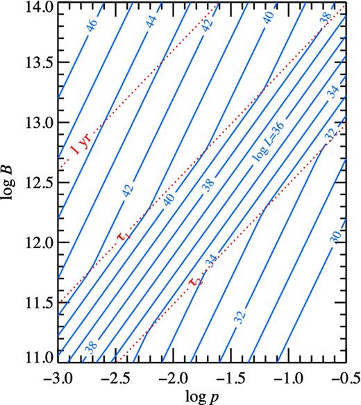
Contour plots of constant X-ray luminosity log L (solid lines) and the characteristic age τc (dotted lines) on the plane magnetic field – period for η0 = 1.
2.2 Steady-state distributions and the differential luminosity function
2.2.1 Steady-state period distribution
2.2.2 Luminosity distribution
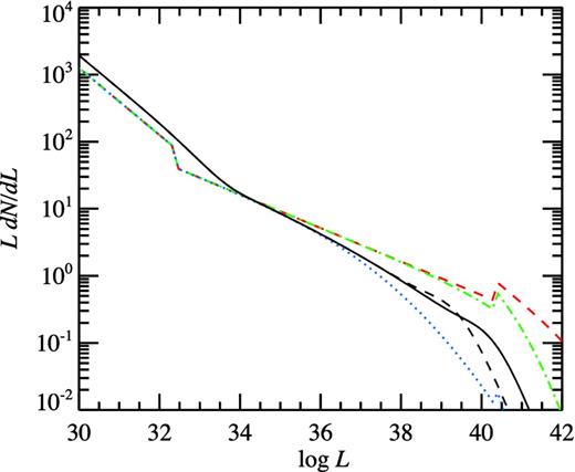
Differential XLF of rotation-powered pulsars for the pulsar birth rate |$\dot{N}_{\rm yr}=0.01$|. The dashed red line shows the XLF for the fixed magnetic field B12 = 4 and very small birth periods with log 〈p0〉 = −2.5 and σp = 0.2. The maximum efficiency is assumed to be η0 = 1. The dash–dotted green line corresponds to the larger birth periods with log 〈p0〉 = −2, and the XLF for even larger log 〈p0〉 = −1.5 is shown by the dotted line. The XLFs averaged over the magnetic field distribution with parameters log 〈B〉 = 12.6 and σB = 0.4 for the birth period distribution parameters log 〈p0〉 = −1.7 and σp = 0.2 are presented by the black solid and dashed lines for the maximum efficiency of η0 = 1 and 0.3, respectively.
The examples of the XLF normalized to the pulsar birth rate |$\dot{N}_{\rm yr}$| are presented in Fig. 2. The XLF has a complex shape reflecting the behaviour of the X-ray radiative efficiency. The XLF for the fixed B has sharp features reflecting breaks in the derivative of the function L(p) given by equation (8). These breaks are unlikely to be observed, because the actual efficiency–age dependence (7) is likely to be smooth.
Radiation from a pulsar may be confined within a narrow beam ∼1 str (Tauris & Manchester 1998) corresponding to the beaming factor b = Ω/4π = 0.1. However, young pulsars have PWN, which are more isotropic. The ratio of the observed luminosities of the nebula to the pulsar has a large spread, but typically is of the order of unity (Kargaltsev & Pavlov 2008). This argues against strong beaming and therefore we take b > 0.3. The normalization of the observed luminosity function scales linearly with the beaming factor.
2.3 Non-stationary solution
2.3.1 Evolution of the period distribution
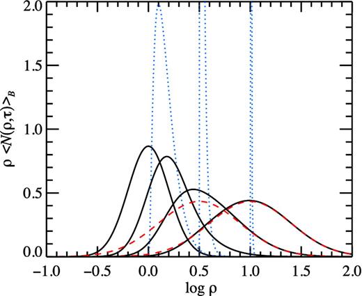
Evolution of the (normalized) period distribution with time. The black solid lines show the evolution of period distribution with initial σp = 0.2 averaged over magnetic field distribution with σB = 0.4 for τ = 0, 1, 10, 100 (from left to right). The blue dotted line shows the period distribution for a specific magnetic field (β = 1) at τ = 1, 10 and 100. The distribution becomes very narrow at large τ, peaking at |$\rho =\sqrt{\tau }$|. The red dashed lines represent the asymptotic solution (37) at large τ, which just reflects the lognormal distribution of the magnetic field.
2.3.2 Evolution of the luminosity distribution
In order to obtain the luminosity distribution, we take the time-dependent solution for the period distribution (26), use the transformation (18) and average the derived expression over the magnetic field. Resulting distribution and its evolution is presented in Figs 4 and 5, respectively. As it is clearly seen from Fig. 4, the initial luminosity distribution of the pulsars can be multimodal. Every mode of the distribution is related to the different regime of the luminosity–period dependence. Also, the luminosity distribution at birth may reveal the narrow spikes, related to the breaks in the |$\text{d}p(L)/\text{d}L$| derivative. The luminosity distribution is broader for larger σp and σB. The distribution becomes narrower and more symmetric as the time increases (Fig. 5). This happens because at birth, pulsars can operate in the different regimes of conversion of the rotational energy losses to the X-ray radiation, depending on the spin period and the magnetic field distributions. With time, all pulsars move towards the same regime, where the efficiency is constant ∼10−4 (see equation 7).
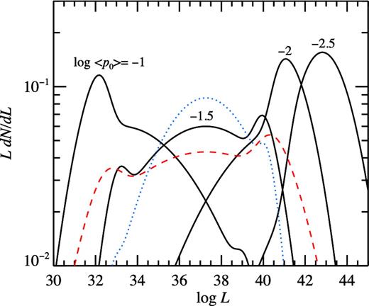
Normalized luminosity distribution at birth for different values of birth period with σp = 0.2, log 〈B〉 = 12.6, σB = 0.4 and η0 = 1 (black lines). The blue dotted and red dashed lines show the luminosity distribution with σB = 0.2 and σp = 0.4, respectively, for log 〈p0〉 = −1.5 (other parameters are the same).
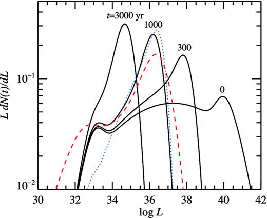
Evolution of the pulsar normalized luminosity distribution for the initial distribution with the following parameters log 〈p0〉 = −1.5, σp = 0.2, log 〈B〉 = 12.6, σB = 0.4 and η0 = 1 (black solid lines). The blue dotted and red dashed lines shows the luminosity distribution at 1000 yr for σB = 0.2 and σp = 0.4, respectively (other parameters are the same). The luminosity distribution becomes more symmetric at large age.
3 OBSERVATIONAL CONSTRAINTS ON MODEL PARAMETERS
3.1 Previous determination of magnetic field and birth period distributions
Distributions of the pulsars over the magnetic field and the birth period were investigated in several papers based on the analysis of the observed radio (Arzoumanian et al. 2002; Faucher-Giguère & Kaspi 2006) and the gamma-ray pulsars (Gonthier et al. 2002; Takata, Wang & Cheng 2011). Parameters of the magnetic field distribution are similar in all these studies lying in the range log 〈B〉 = 12.35–12.75, σB=0.1–0.55 (see Table 1). However, parameters of the birth period distributions are significantly different: the mean logarithm log 〈p0〉 varies from −2.3 to −0.5 (i.e. periods in the range from 5 to 200 ms) and the width σp varies in the range 0–0.8 (see Table 1; the parameters were estimated by fitting the lognormal distribution to the actual distributions adopted by the authors). This difference in the birth period distributions is most likely caused by a low sensitivity of the considered models to the birth period. As it was shown on Section 2, the period distribution of the pulsars at large time does not contain information about the birth periods. Therefore, in order to determine these parameters we have to use only young pulsars.
Birth rates and parameters of the magnetic field and the birth period distributions for rotation-powered pulsars.
| Model | log 〈p0〉 | σp | log 〈B〉 | σB | |$\dot{N}_{\rm yr}$|a | Referenceb |
|---|---|---|---|---|---|---|
| 1 | −2.3 | 0.3c | 12.35 | 0.4 | 0.0013 | 1 |
| 2 | −1.52 | 0.0 | 12.75d | 0.33d | 0.01e | 2 |
| 3 | −0.52f | 0.8f | 12.65 | 0.55 | 0.028g | 3 |
| 4 | −1.7h | 0.1h | 12.6 | 0.1 | 0.01 | 4 |
| Model | log 〈p0〉 | σp | log 〈B〉 | σB | |$\dot{N}_{\rm yr}$|a | Referenceb |
|---|---|---|---|---|---|---|
| 1 | −2.3 | 0.3c | 12.35 | 0.4 | 0.0013 | 1 |
| 2 | −1.52 | 0.0 | 12.75d | 0.33d | 0.01e | 2 |
| 3 | −0.52f | 0.8f | 12.65 | 0.55 | 0.028g | 3 |
| 4 | −1.7h | 0.1h | 12.6 | 0.1 | 0.01 | 4 |
aBirth rate of pulsars in the Milky Way per year.
bReferences: (1) Arzoumanian et al. (2002); (2) Gonthier et al. (2002); (3) Faucher-Giguère & Kaspi (2006); (4) Takata et al. (2011).
cReference 1 gives the lower limit on σp of 0.2. Taking a broader distribution with σp > 0.3 does not affect the results.
dParameters for the lognormal distribution were estimated by fitting a more complex distribution adopted in Reference 2, see their table 1 and equation 1.
eValue from the first line of Table 8 of Reference 2.
fParameters for the lognormal distribution were estimated by fitting a Gaussian distribution adopted in Reference 3, see their table 8.
gBirth rate from table 8 of Reference 3.
hThe lognormal distribution approximates the flat distribution in the 20–30 ms range adopted in Reference 4.
Recently, Popov & Turolla (2012) have presented new estimates of the birth periods based on a sample of radio pulsars associated with the SN remnants. They showed that the distribution has to be rather wide, and it is consistent with a Gaussian with the mean p0 ∼ 0.1 s and width σ ∼ 0.1 s. However, this result is inconclusive, because the number of objects in the used sample is not large enough to derive the exact shape of the period distribution.
The analysis of the observed luminosity distribution of the historical core-collapse SNe by Perna et al. (2008) showed that the predicted number of bright pulsars in the Perna & Stella (2004) model is much larger than the observed number of luminous SNe. This discrepancy is related to the assumed very short (5 ms) mean birth period from Arzoumanian et al. (2002). On the other hand, using parameters of the pulsar magnetic field distribution from Faucher-Giguère & Kaspi (2006), Perna et al. (2008) found that in order to satisfy the observed luminosity distribution of the historical core-collapse SNe, the birth period of the pulsars should be larger than 40–50 ms.
In the following sections, we repeat the analysis by Perna et al. (2008) using a different efficiency–age dependence given by equation (7) as well as using the new data that became available after 2008. We also obtain constraints on the pulsar birth period distribution by comparing the simulated pulsar XLF with the observed XLF of the bright sources in the nearby galaxies derived by Mineo, Gilfanov & Sunyaev (2012).
3.2 Constraints from the luminosity distribution of core-collapse SNe
Perna et al. (2008) proposed that constraints on the birth period distribution can be obtained by comparing the observed luminosity distribution of historical core-collapse SNe with the simulated pulsar XLF (for the given ages), considering that the most probable remnant of the core-collapse SN explosion is a neutron star.
The second issue is the fallback accretion on to a neutron star during early phases of SN explosion. According to Chevalier (1989), radiation from the central pulsar begins to diffuse through the accreting matter when a reverse shock radius reaches the radiation trapping radius. It happens at ≳0.5 yr after the SN. Therefore, we can expect that the central pulsars will contribute to the total luminosity after 0.5–1.0 yr. This estimate is close to the limit coming from the diffusion time arguments. Thus, we will use the minimal age t = 0.5 yr.
Another important question is a selection effect, which may strongly affect the observed luminosity distribution of SNe, because the younger is the source the brighter it is and the higher is the probability for it to be detected. For example, most of the SNe luminosity measurements from Perna et al. (2008) are upper limits, because those sources are quite faint. Only 19 brightest and youngest sources have actual measurements of luminosity. Compilation of Dwarkadas & Gruszko (2012) contains additional 11 sources with known luminosity, but there are only four sources with ages >0.5 yr. In addition, because some fraction of the SNe X-ray luminosity is not related to the pulsar or PWN, also the actual X-ray detections here should be treated as upper limits on the pulsar luminosity. For the analysis, we use the data on the ages and the X-ray luminosities of core-collapse SNe (with ages >0.5 yr) from Perna et al. (2008) with the addition of the new measurements from the compilation of Dwarkadas & Gruszko (2012) (see Tables 2 and 3). The cumulative histogram of upper limits is shown in Fig. 6 by the bold pink line.
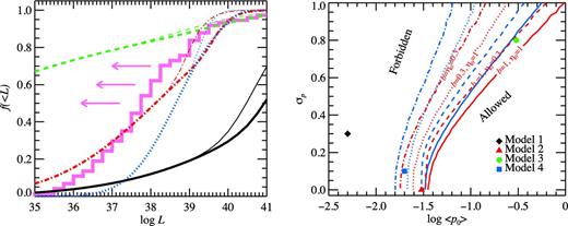
(a) Cumulative normalized luminosity distributions for SNe (either measurements or upper limits; pink histogram) with ages t > 0.5 yr. The black solid, red dash–dotted, green dashed and blue dotted lines correspond to average distributions for models 1–4 from Table 1, respectively. Thick lines are for the case η0 = 1 and the thin lines are for η0 = 0.3. Here, no beaming is assumed (b = 1). (b) Allowed region for the parameters of the birth period distribution. Parameters along the red and blue lines satisfy condition (42) in 90 and 68 per cent cases, respectively. The solid, dashed, dotted and dot–dashed lines correspond to different pairs of (b, η0) = (1,1), (1,0.3), (0.3,1) and (0.3,0.3), respectively. Regions to the right of these lines satisfy the data with higher probability. The calculations are performed for the average values of the magnetic field distribution log 〈B〉 = 12.6 and σB = 0.4. The positions of parameters listed in Table 1 are marked by different symbols.
X-ray luminosities of historical SNe.
| SN | Age (yr)a | log L | Referencesb |
|---|---|---|---|
| 1979C | 26.8 | 38.43|${^{+ 0.06}_{- 0.07}}$| | 1 |
| 1986E | 19.6 | 38.15|${^{+ 0.13}_{- 0.19}}$| | 1 |
| 1986J | 21.2 | 38.93|${^{+ 0.02}_{- 0.03}}$| | 1 |
| 1988Z | 15.5 | 39.46|${^{+ 0.07}_{- 0.08}}$| | 1 |
| 1990U | 10.9 | 39.04|${^{+ 0.19}_{- 0.26}}$| | 1 |
| 1994I | 8.2 | 36.90|${^{+ 0.02}_{- 0.04}}$| | 1 |
| 1995N | 8.9 | 39.63|${^{+ 0.09}_{- 0.11}}$| | 1 |
| 1996cr | 4.2 | 39.28|${^{+ 0.08}_{- 0.10}}$| | 1 |
| 1998S | 3.6 | 39.58|${^{+ 0.05}_{- 0.06}}$| | 1 |
| 1998bw | 3.5 | 38.60|${^{+ 0.10}_{- 0.11}}$| | 1 |
| 1999ec | 5.9 | 39.49|${^{+ 0.05}_{- 0.06}}$| | 1 |
| 2001em | 4.7 | 40.76|${^{+ 0.08}_{- 0.10}}$| | 1 |
| 2001gd | 1.1 | 39.00|${^{+ 0.11}_{- 0.15}}$| | 1 |
| 2001ig | 0.5 | 37.54|${^{+ 0.20}_{- 0.37}}$| | 1 |
| 2004C | 3.1 | 38.00|${^{+ 0.11}_{- 0.10}}$| | 1 |
| 2005ip | 1.3 | 40.20|${^{+ 0.07}_{- 0.09}}$| | 2 |
| 2005kd | 1.2 | 41.41|${^{+ 0.06}_{- 0.07}}$| | 1 |
| 2006jd | 1.1 | 41.40|${^{+ 0.12}_{- 0.17}}$| | 3,4 |
| 2008ij | 0.56 | 39.00|${^{+ 0.11}_{- 0.15}}$| | 5 |
aAges of SNe were calculated from the detection times listed at the website of the IAU Central Bureau for Astronomical Telegrams, except for SNe from Perna et al. (2008).
Upper limits for the X-ray luminosities of historical SNe (from Perna et al. 2008).
| SN | Age (yr) | log L |
|---|---|---|
| 1923A | 77.3 | 35.78 |
| 1926A | 75.3 | 37.15 |
| 1937A | 67.3 | 37.11 |
| 1937F | 62.1 | 36.43 |
| 1940A | 63.0 | 37.00 |
| 1940B | 62.6 | 36.93 |
| 1941A | 60.2 | 36.74 |
| 1948B | 55.1 | 35.67 |
| 1954A | 48.9 | 35.20 |
| 1959D | 41.6 | 37.34 |
| 1961V | 38.3 | 37.79 |
| 1962L | 41.2 | 37.67 |
| 1962M | 40.3 | 35.57 |
| 1965H | 37.7 | 38.18 |
| 1965L | 37.8 | 36.76 |
| 1968L | 32.0 | 36.18 |
| 1969B | 32.6 | 36.58 |
| 1969L | 30.3 | 37.68 |
| 1970G | 33.9 | 36.69 |
| 1972Q | 30.5 | 38.48 |
| 1972R | 31.9 | 35.86 |
| 1973R | 25.9 | 37.89 |
| 1976B | 26.2 | 37.95 |
| 1980K | 24.0 | 36.81 |
| 1982F | 22.6 | 36.04 |
| 1983E | 19.0 | 37.66 |
| 1983I | 17.8 | 36.23 |
| 1983N | 16.8 | 36.74 |
| 1983V | 19.1 | 37.85 |
| 1985L | 14.9 | 37.91 |
| 1986I | 17.1 | 38.48 |
| 1986L | 18.9 | 38.15 |
| 1987B | 14.1 | 38.18 |
| 1988A | 12.3 | 37.38 |
| 1991N | 11.8 | 37.62 |
| 1993J | 8.1 | 38.00 |
| 1994ak | 7.4 | 37.57 |
| 1996ae | 5.9 | 37.79 |
| 1996bu | 6.6 | 37.32 |
| 1997X | 6.1 | 37.34 |
| 1997bs | 2.5 | 38.46 |
| 1998T | 5.2 | 38.30 |
| 1999dn | 4.4 | 37.77 |
| 1999el | 5.6 | 38.75 |
| 1999em | 1.0 | 37.15 |
| 2000P | 7.2 | 39.08 |
| 2000bg | 1.3 | 39.15 |
| 2001ci | 2.5 | 37.70 |
| 2001du | 1.3 | 37.58 |
| 2002ap | 0.9 | 36.49 |
| 2002fjn | 4.7 | 39.11 |
| 2002hf | 3.1 | 38.88 |
| 2003dh | 0.7 | 40.70 |
| 2005N | 0.5 | 40.00 |
| 2005at | 1.7 | 38.48 |
| 2005bf | 0.6 | 39.78 |
| 2005gl | 1.6 | 39.53 |
We follow the recipe described in Section 2.3.2 and calculate the luminosity distribution of 76 pulsars for the ages of SNe listed in Tables 2 and 3. We then construct the average normalized cumulative distribution of luminosities f ( < L) and compare it to the observed distribution. In the absence of beaming (i.e. b = 1), from Fig. 6(a), we see that only model 3 (Faucher-Giguère & Kaspi 2006) satisfies the upper limit distribution, for the maximum efficiency η0 between 0.3 and 1. Model 2 (Gonthier et al. 2002) is also reasonably close, especially for η0 = 0.3.
An additional effect appears if beaming is significant. Then most of the pulsars which appear to be faint in the X-rays, in reality could be very bright sources, but beamed away from us. Furthermore, about 10 per cent of SNe produce a black hole after explosion instead of a neutron star (Heger et al. 2003), which can be modelled as an additional multiplicative beaming factor 0.9. The cumulative normalized luminosity function in that case would start from the value 1 − 0.9b at the low-luminosity end. For example, for a smaller beaming factor b = 0.3, most of the bright pulsars would be undetected. In that case, models 2 and 3 satisfy the upper limit distributions, model 4 is only marginally consistent with them, but model 1 (Arzoumanian et al. 2002) still contradicts the data.
consistent with those derived by Perna et al. (2008), who found 〈p0〉 >40–50 ms.
3.3 Constraints from the XLF for sources in nearby galaxies
3.3.1 Averaged XLF of nearby galaxies
3.3.2 Comparisons of the pulsar and observed XLF
In order to make the comparisons between the pulsar XLF and the observed XLF of sources in the nearby galaxies, we first need to find the relation between the pulsar birth rate and the SFR. We assume the Galactic SFRMW = 2 M⊙ yr−1, in accordance with the recent study of Chomiuk & Povich (2011). However, using luminous radio SN remnants and the X-ray point sources, these authors found that the Milky Way deviates from SFR expectations at the 1–3σ level, hinting that the Galactic SFR is overestimated or extragalactic SFRs need to be revised upward.
Using the conversion formula (45), we can now produce the cumulative luminosity distribution of pulsars normalized by the SFR and compare it to the observed XLF from Mineo et al. (2012). The XLFs calculated for the four models from Table 1 are presented in Fig. 7a. We see that all cumulative XLF are harder than the observed XLF at luminosities below 1038 erg s−1. This fact is easy to understand from our Fig. 2 and equation (21): the typical slope of 1.25 is related to the intermediate characteristic ages (see equation 7), where the efficiency varies strongly. The position of the cutoff depends not only on the mean birth period, but also on the width of the distribution. For example, model 3 has the largest mean period, but because of a large dispersion, the XLF extends to very high luminosities without a visible break. On the other hand, model 2 has a rather small mean period, but the XLF cuts off sharply, because of the zero σp and the absence of fast pulsars. Model 1 has the largest number of bright pulsars because of the smallest mean period (see also Fig. 2). Model 4 also shows a cutoff at rather small luminosity in spite of the small initial periods, because of the narrow magnetic field distribution.
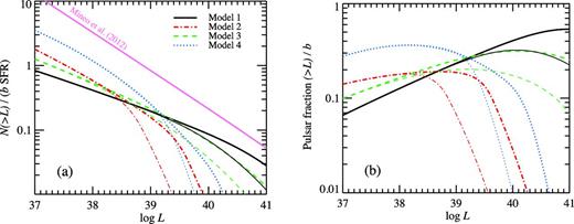
(a) Cumulative luminosity distribution of the pulsars normalized to the unit SFR and unit beaming b = 1. The black solid, red dash–dotted, green dashed and blue dotted lines correspond to models 1–4, respectively. The thick and thin lines correspond to the maximum efficiency of η0 = 1 and 0.3, respectively. The pink solid straight line represents the average cumulative XLF of sources in the nearby galaxies (Mineo et al. 2012) taken in the form (44). (b) The predicted fraction (above a given luminosity) of pulsars in the high-luminosity end of the average XLF. Each line corresponds to the same models as in panel (a).
The number of high-luminosity pulsars depends on the maximum efficiency η0. Decreasing η0 leads to a smaller cutoff luminosity (compare thick and thin curves in Fig. 7a). However, if the cutoff is at very large luminosity (as e.g. in the case of models 1 and 3), variations in η0 do not affect significantly the observed XLF, at least in the range of luminosities log L < 40. The XLF normalization scales linearly with the beaming factor b.
Dividing the pulsar cumulative XLF by the observed XLF, we obtain the fraction of pulsars as a function of luminosity. It is an increasing function of luminosity and reaches the maximum at log L between 38 and 41, depending on the model parameters, see Fig. 7(b). The maximum pulsar fraction reaches (0.2–0.5)b for all models.
3.3.3 Constraints on the birth period distribution
For a smaller value of the maximal efficiency η0 = 0.3, the critical line (red bold dashed line in Fig. 8) shifts to the left and depends weaker on σp. Thus, the decrease of the efficiency leads to shorter allowed periods. Variations in the beaming factor lead to a stronger effect. For b = 0.3 and η0 = 1, the allowed region extends beyond the parameters from Takata et al. (2011), but still cannot reach the parameters from Arzoumanian et al. (2002).
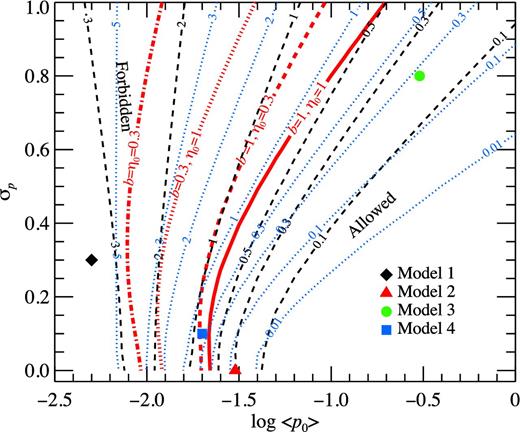
Allowed region for the parameters of the birth period distribution derived from the XLF of sources in the nearby galaxies and the fraction of pulsars in the observed cumulative XLF (Mineo et al. 2012). Parameters along the bold red lines satisfy equation (46). The solid, dashed, dotted and dot–dashed lines correspond to different pairs of (b, η0) = (1,1), (1,0.3), (0.3,1) and (0.3,0.3), respectively. The regions to the right of these lines are allowed and to the left are forbidden. The dashed black and dotted blue contours give the pulsar fraction for b = 1 at luminosities above 1039 and 1040 erg s−1, respectively. Calculations are performed for the average values log 〈B〉 = 12.6, σB = 0.4 and κ = 0.01. The positions of parameters listed in Table 1 are marked by different symbols.
We note here that for simulations we used the average value of the pulsar birth rate κ = 0.01, while it is more than 10 and two times smaller in models of Arzoumanian et al. (2002) and Takata et al. (2011), respectively. Thus, all considered models are in principle allowed if one corrects for different κ. However, for small b and η0 the constraints coming from the SNe (see Fig. 6b) are actually stronger and rule out model 1, with model 4 being only marginally consistent with the data.
4 PULSAR CONTRIBUTION TO ULX
4.1 Dependence on the birth period distribution
We can also calculate the pulsar fraction dependence on the combination (log 〈p0〉, σp). This fraction calculated for sources with luminosities log L > 39 and >40 is presented as contours in Fig. 8. We see that the models 2 and 3 lie nearly on the same curve. The explicit dependence of the pulsar fraction on the parameters of the birth period distribution is shown in Fig. 9. We see that for small initial mean periods, the pulsar fraction is nearly independent of σp because the XLF cuts off at very high luminosities. The situation changes dramatically at large 〈p0〉: the narrow period distribution now predicts cutoff at low luminosity and the pulsar fraction is negligible. At large widths σp ∼ 1, the pulsar fraction is still large because of the large extent of the XLF. Situation is similar for the cutoff luminosity log L = 40, but now for small σp the XLF cuts off close to the limiting luminosity even for rather short initial periods and the pulsar fraction is small in that case. For large σp ∼ 1, the pulsar fraction exceeds that fraction for log L = 39 if log 〈p0〉 ≲ −0.5.
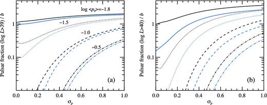
The fraction of the pulsars in the observed cumulative XLF (Mineo et al. 2012) at luminosities above 1039 erg s−1 (panel a) and above 1040 erg s−1 (panel b) (see Section 4.1) as a function of σp. The solid, dotted, dashed and dot–dashed lines correspond to the mean period of log 〈p0〉 = −1.8, −1.5, −1.0 and 0.5, respectively. The upper black and the lower blue lines give the pulsar fraction for η0 = 1 and 0.3, respectively. Calculations are performed for the values log 〈B〉 = 12.6, σB = 0.4 and κ = 0.01.
4.2 Dependence on the maximum efficiency
In a general case, the dependence of the pulsar fraction above log L = 39 on η0 can be easily seen in Fig. 9a. For small initial periods, the pulsar fraction is nearly independent of η0 for all σp because the XLF extends to very high luminosities. For larger initial mean periods, the dependence on η0 is strong for narrow distributions σp ∼ 0, because the XLF has a sharp cutoff around log L = 39. For broad initial distributions with σp ∼ 1, the pulsar fraction is still rather large and the dependence on η0 is not so strong.
The pulsar fraction at luminosities in excess of log L = 40 (see Fig. 9b) shows a similar behaviour, but dependence on η0 is stronger because typically the XLF cuts off at that luminosity even for small initial periods and large σp.
The dependence of the pulsar fraction on the maximum efficiency η0 for the models listed in Table 1 is presented in Fig. 10. Most of the models predict rather flat dependence on η0 of the pulsar fraction at log L > 39 because of the wide initial period distribution producing the XLF extending to rather high luminosities. The only exception is model 2 (Gonthier et al. 2002), which predicts a significant drop in the pulsar function below η0 = 0.5. This is a direct consequence of the fact that this model has a narrow period distribution and its XLF has a sharp cutoff at about log L = 39.3 for η0 = 1.0. Thus, we see that for a rather wide range of η0 between 0.3 and 1 the pulsar fraction above log L = 39 is between about 10 and 30 per cent for all models. Obviously, the beaming can reduce this fraction proportionally and for b = 0.3 it is then at least 3 per cent.
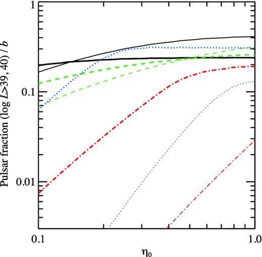
The predicted fraction of pulsars at luminosities above 1039 erg s−1 (thick lines) and above 1040 erg s−1 (thin lines) in the average XLF of sources in the nearby galaxies (Mineo et al. 2012) taken in the form (43) as a function of the maximum efficiency. The black solid, blue dotted, red dot–dashed and green dashed curves correspond to models 1–4 from Table 1, respectively.
For models 1 and 3, the pulsar fraction is even larger at very high luminosities in excess of log L = 40 reaching 0.4b and 0.3b, respectively. In those cases, the dependence on η0 is also not strong. While for model 2, the pulsar fraction is below 3 per cent and scales approximately as η|${^{2}_{0}}$|. From Fig. 8 it is clear that the closer parameters of the birth periods are to the limiting (bold red) line, the larger is the pulsar fraction. For large σp, the cumulative XLF is less steep than the observed XLF and therefore the pulsar fraction is a monotonically growing function that can reach 100 per cent above log L = 40. Thus, it is possible that the pulsar fraction among the brightest ULX is significantly larger than 10 per cent.
4.3 Distribution functions of the luminous pulsars
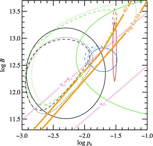
Distribution of pulsars over magnetic field and initial periods. The black, red, green and blue solid curves encircle 90 per cent of pulsars for models 1–4 from Table 1, respectively. The dotted and dashed curves encircle 90 per cent of initial pulsar distribution that can be observed to radiate above 1039 erg s−1 and 1040 erg s−1, respectively. The mean and the standard deviation describing these distributions are given in Table 4. The dotted pink curves give the dependence τc = τ1 and τc = τ2. The solid brown curves are the lines of constant X-ray luminosity of 1039 and 1040 erg s−1 for η0 = 1.
These density distributions of the bright observed pulsars for various models from Table 1 are shown in Fig. 11. These distributions are generally narrower than the original distribution and skewed towards smaller periods and larger magnetic fields. They are elongated along the line of constant luminosity. The mean values and the standard deviations of these distributions are given in Table 4. We also find the distribution of true ages of these pulsars, which is a monotonically decreasing function and can be described by the median age τ.
Parameters of the birth period and the magnetic field distributions as well as the median true age of pulsars with observed luminosities in excess of a given value for models from Table 1.
| Model | log 〈p0〉 | σp | log 〈B〉 | σB | τ |
|---|---|---|---|---|---|
| yr | |||||
| log L > 39 | |||||
| 1 | −2.43 | 0.24 | 12.35 | 0.34 | 343 |
| 2 | −1.52 | 0.0 | 13.13 | 0.16 | 96 |
| 3 | −2.05 | 0.39 | 12.79 | 0.44 | 136 |
| 4 | −1.80 | 0.08 | 12.67 | 0.09 | 105 |
| log L > 40 | |||||
| 1 | −2.46 | 0.23 | 12.39 | 0.32 | 174 |
| 2 | −1.52 | 0.0 | 13.37 | 0.13 | 13 |
| 3 | −2.22 | 0.34 | 12.71 | 0.41 | 52 |
| 4 | −1.86 | 0.07 | 12.70 | 0.08 | 36 |
The evolution of the luminosity for the average luminous pulsar can be described as follows: during the first ten years the luminosity is nearly constant at the level of ∼1040 erg s−1. After that it starts to decrease and still exceeds ∼1039 erg s−1 for the next 100 yr, during which the pulsars can be observed as ULXs. After that the luminosity decreases down to ∼1036 erg s−1 in about 1000 yr.
The rotation-powered pulsars are often assumed to be non-variable sources, but there may exist some variability on the time-scales shorter that ∼100 yr related to the interaction of the SN remnant with the PWN and the surrounding media. As it was shown by Dwarkadas & Gruszko (2012), the SN remnant could show a variability at least on the time-scales ∼10 yr. This variability could depend on the scale and the spatial spectrum of inhomogeneities of the surrounding media, and the characteristic variability time-scale may increase with the pulsar age. The spectrum in the 0.1–10 keV range should consist of the soft thermal component related to the shock and the power-law tail related to the synchrotron radiation both from the shocks and the central pulsar.
5 SUMMARY
In this paper, we have investigated the question whether rotation-powered pulsars and PWN could be observed as some subclass of ULXs, and, if it is so, what is the fraction of pulsars in the whole ULX population.
First, we developed an analytical model of the XLF, by solving the evolution equation for the period distribution of the pulsars. We derived both the steady-state and the time-dependent solution. The steady-state solution is transformed to the pulsar XLF. We showed that this XLF has a broken power-law shape, reflecting the complex behaviour of the efficiency, with the high luminosity cut-off which location and shape are determined by the parameters of the birth period and magnetic field distributions. The location of the cutoff mainly depends on the mean birth period. For short enough birth periods, the cutoff may lie above 1039 erg s−1. Therefore, the existence of luminous pulsars is possible.
The time-dependent solution tells us about the evolution of the distribution functions of the pulsars. We have shown that at large ages the period distribution becomes a delta-function-like peaking at |$\sqrt{\alpha t}B$|. The time-dependent luminosity distribution is more complicated due to the complexity of the luminosity–period relation. It can be multimodal with different modes related to the different regimes of the efficiency of conversion of the rotation energy losses to the X-ray radiation. As the age of the pulsars increases, the luminosity distribution becomes more symmetric.
We found constraints on the parameters of the birth period distribution using the observed XLF of the sources in the nearby galaxies obtained by Mineo et al. (2012). We found that the mean birth period cannot be shorter than 10–30 ms, depending on the width of the distribution. Therefore, the parameters derived by Arzoumanian et al. (2002) lie in the forbidden region for the typically assumed pulsar production rates. Accounting for the recent findings of Popov & Turolla (2012), the parameters obtained by Faucher-Giguère & Kaspi (2006) are the most reliable.
We discussed the influence of the beaming and the maximal efficiency on the luminosity function. For our calculations, we assumed conservatively b > 0.3, but the results can be easily scaled to the different values of the beaming. The number of the observed pulsars and their contribution to the ULX population depend linearly on b. The influence of the maximal efficiency is more complex, because it affects only the high luminosity tail of the pulsar XLF. For η0 = 0.3 the allowed parameter space of the birth period distribution expands towards the shorter birth periods. The fraction of pulsars in the observed XLF of Mineo et al. (2012) would be smaller for smaller values of the efficiency and it strongly depends on the luminosity above which this fraction is computed. We showed that for broad initial period distributions, the pulsar fraction is a weak function of η0.
We have also obtained constraints on the period distribution by applying the method proposed by Perna et al. (2008). We derived the luminosity function of core-collapse SNe, using published X-ray light curves and compared it to the time-dependent luminosity function for pulsars. We found that the observed luminosities of the SNe are consistent with the mean birth period of p0 ≳ 0.015–1 s, depending on the width of the distribution, maximum efficiency and the beaming factor. These constraints are in agreement with those derived by Perna et al. (2008).
We estimated a possible fraction of the pulsars in the whole population of ULX, using the observed XLF from Mineo et al. (2012). For the models considered in the previous studies of pulsar populations, the predicted fraction of luminous pulsars can be in excess of 3 per cent for the sources with luminosities greater than 1039 erg s−1. At this moment, about 500 ULXs have been discovered (Feng & Soria 2011; Swartz et al. 2011; Walton et al. 2011) and we expect that at least ∼15 of those should be associated with the rotation-powered pulsars. The models predict the pulsar fraction above 1040 erg s−1 at the level of 1–40 per cent.
Therefore, we might potentially observe bright pulsars as ULXs in galaxies with high SFR. These pulsars should have almost constant luminosity during the first hundred years after their birth, but there may exist some variability on the time-scale of ∼10 yr related to the interaction of the expanding SN remnant shell with the surrounding media.
The research was supported by the Academy of Finland grant 127512.
