


ABSTRACT
We analyse current measurements of accretion rates on to pre-main-sequence stars as a function of stellar mass, and conclude that the steep dependence of accretion rates on stellar mass is real and not driven by selection/detection threshold, as has been previously feared. These conclusions are reached by means of statistical tests including a survival analysis which can account for upper limits. The power-law slope of the Ṁ–M* relation is found to be in the range of 1.6–1.9 for young stars with masses lower than 1 Mȯ. The measured slopes and distributions can be easily reproduced by means of a simple disc model which includes viscous accretion and X-ray photoevaporation. We conclude that the Ṁ–M* relation in pre-main-sequence stars bears the signature of disc dispersal by X-ray photoevaporation, suggesting that the relation is a straightforward consequence of disc physics rather than an imprint of initial conditions.
1 INTRODUCTION
The scaling of the accretion rate, |$\skew3\dot{M}$|, with stellar mass, M* for low-mass stars has been the focus of much debate over the last few years. Measurements in the first half of the naughties, indicated that |$\skew3\dot{M}$| correlates with the square of the stellar mass (Muzerolle et al. 2003, 2005; Calvet et al. 2004; Natta et al. 2004; Mohanty, Jayawardhana & Basri 2005; Natta, Testi & Randich 2006). This deviation from a simple linear scaling encouraged the development of a number of theoretical models to interpret these results, including Bondi–Hoyle accretion (Padoan et al. 2005, see also Throop & Bally 2008) and dependence on the initial conditions of the parent cloud from which the protoplanetary disc formed (Alexander & Armitage 2006; Dullemond, Natta & Testi 2006). Clarke & Pringle (2006, hereafter CP06) and later Tilling et al. (2008), questioned the quantitative value of the power-law exponent, α, in the |$\skew3\dot{M}{\rm -}M_*$| relation, suggesting that incompleteness of the data at both high and low accretion rates may have conspired to yield a higher than expected value of α. By considering disc dispersal by EUV photoevaporation, CP06 derive a theoretical value of α = 1.35. A similar slope was also obtained by an independent model of Gregory et al. (2006) based on a steady state accretion which considered both dipolar and complex magnetic fields.
Recent observational data, however, lend credence to higher values of the α exponent. Using different observational methods and samples in different regions, the typical derived values of α are around 1.5–1.8 (e.g. Herczeg & Hillenbrand 2008; Antoniucci et al. 2011; Rigliaco et al. 2011; Biazzo et al. 2012). In particular, Manara et al. (2012) used the Hubble Space Telescope (HST) to investigate the |$\skew3\dot{M}{\rm -}M_*$| relation in the Orion nebula cluster, finding a value of α = 1.68 ± 0.02 (compatible with the results of Natta et al. 2006). Selecting sources according to the method used for the determination of the accretion rates in the same sample returns values varying from α = 1.59 ± 0.04 to 1.73 ± 0.02.
In this paper, we show that values of α ∼ 1.45–1.70 are expected for stars with solar mass or lower, in the context of a protoplanetary disc dispersal mechanism based on X-ray photoevaporation. The work is organized as follows. In Section 2, we describe the available observational data and perform some simple survival statistics to account for upper limit measurements. In Section 3, we describe the theoretical prediction of the |$\skew3\dot{M}{\rm -}M_*$| relation for a population of discs dispersed by X-ray photoevaporation, showing that this agrees with the observational values and perform additional statistical tests. In Section 4, we briefly summarize our findings.
2 OBSERVATIONAL SAMPLES
We have collected mass accretion rates versus stellar mass data from the literature in order to investigate the correlation between |$\skew3\dot{M}$| and M* implied by recent observational data. Our data set is described in Table 1. In order to address the concern raised by CP06, that the steepness of the |$\skew3\dot{M}{\rm -}M_*$| relation may be driven by selection effects in the data, we have collected, where available, all upper limits and included them in the calculation of α by means of survival statistics techniques. The total number of data points we have collected is 3764 of which 15.4 per cent are upper limits. Necessarily a number of measurements are duplicated in various sources, namely 84.1 per cent are duplicates. In such cases, we have taken the geometrical average of the measurements. In cases where both measurements and upper limits are available for an individual source we neglect the upper limits and only use the measurements. Binaries are a further source of contamination, around 7 per cent of the objects in the total sample are in known systems, but it is unclear how many unknown binaries may still be left. In total, we are left with 1623 measurements for individual objects of which 294 are upper limits. A plot of the full data set is shown in Fig. 1.
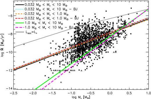
Accretion rates as a function of stellar mass for the whole collected sample. Crosses represent measurements and triangles upper limits. The slopes of the distributions are listed in Table 2. The grey solid line shows the locus where the accretion and bolometric luminosity are equal.
Regions and references of acquired sample.
| Region | No. of measurements | No. of upper limits | Methodsa | References |
|---|---|---|---|---|
| ASSOC II SCO + ASS Sco OB + | 10 | 4 | a, b, c | Total |
| LCC + USco | 1 | 0 | a, b | Curran et al. (2011) |
| 4 | 3 | a, c | Herczeg, Cruz & Hillenbrand (2009) | |
| 0 | 1 | a | Mohanty et al. (2005) | |
| 5 | 1 | a | Garcia Lopez et al. (2006) | |
| Cra dark cloud | 2 | 3 | a | Total |
| 2 | 2 | a | Fang et al. (2013) | |
| 0 | 1 | a | Garcia Lopez et al. (2006) | |
| Cep OB2 Tr37 + Cep OB2 NGC 7160 | 90 | 10 | d | Total |
| 81 | 1 | d | Sicilia-Aguilar, Henning & Hartmann (2010) | |
| 35 | 27 | d | Sicilia-Aguilar et al. (2006) | |
| Cha I + Cha II | 82 | 15 | a, d, e | Total |
| 2 | 7 | a, e | Natta et al. (2004) | |
| 6 | 12 | e | Muzerolle et al. (2005) | |
| 10 | 1 | a | Costigan et al. (2012) | |
| 4 | 0 | a | Fang et al. (2013) | |
| 16 | 0 | d | Hartmann et al. (1998) | |
| 0 | 2 | a | Mohanty et al. (2005) | |
| 18 | 0 | a | Robberto et al. (2012) | |
| 37 | 0 | a | Biazzo et al. (2012) | |
| IC 348 | 19 | 3 | a, e, f | Total |
| 6 | 0 | e | Muzerolle et al. (2003) | |
| 4 | 2 | a | Mohanty et al. (2005) | |
| 13 | 1 | a, f | Dahm (2008) | |
| L1630N | 70 | 0 | a | Fang et al. (2009) |
| L1641 | 103 | 0 | a | Fang et al. (2009) |
| Lupus | 5 | 2 | a, b, c | Total |
| 3 | 2 | a | Fang et al. (2013) | |
| 1 | 0 | a, b | Curran et al. (2011) | |
| 1 | 0 | c | Herczeg & Hillenbrand (2008) | |
| 1 | 0 | a | Garcia Lopez et al. (2006) | |
| Orion nebular cluster | 698 | 85 | a, g | M12 |
| TWA | 6 | 2 | a, b, c, e | Total |
| 1 | 1 | c, e | Muzerolle et al. (2000) | |
| 1 | 0 | a | Donati et al. (2011a) | |
| 2 | 0 | a, b | Curran et al. (2011) | |
| 3 | 0 | c, e | Herczeg & Hillenbrand (2008) | |
| 4 | 1 | c | Herczeg et al. (2009) | |
| 0 | 1 | a | Mohanty et al. (2005) | |
| σ Orionis | 39 | 45 | a, c, d | Total |
| 6 | 2 | c | Rigliaco et al. (2012) | |
| 12 | 23 | a | Gatti et al. (2008) | |
| 30 | 30 | d | Rigliaco et al. (2011) | |
| ε Cha | 4 | 0 | a | Fang et al. (2013) |
| Taurus | 118 | 40 | a, b, c, d, e, f | Total |
| 17 | 0 | c | Gullbring et al. (1998) | |
| 6 | 1 | c, e | Muzerolle et al. (2003) | |
| 9 | 6 | e | Muzerolle et al. (2005) | |
| 55 | 25 | f | White & Ghez (2001) | |
| 40 | 0 | c, d | Hartmann et al. (1998) | |
| 2 | 0 | a, b | Curran et al. (2011) | |
| 16 | 2 | c, e | Herczeg & Hillenbrand (2008) | |
| 6 | 3 | a | Mohanty et al. (2005) | |
| 1 | 0 | f | White & Hillenbrand (2005) | |
| 3 | 7 | f | White & Basri (2003) | |
| 23 | 3 | f | White & Hillenbrand (2004) | |
| ρ Oph | 46 | 72 | a, e | Total |
| 46 | 71 | a | Natta et al. (2006) | |
| 7 | 3 | a, e | Natta et al.(2004) | |
| 13 | 3 | a | Gatti et al. (2006) | |
| 1 | 0 | a | Donati et al. (2011b) | |
| 1 | 0 | a | Curran et al. (2011) | |
| 1 | 1 | a | Mohanty et al. (2005) | |
| Various | 28 | 7 | a, b | Total |
| 6 | 3 | a | Fang et al. (2013) | |
| 1 | 0 | a | Mohanty et al. (2005) | |
| 20 | 4 | a | Garcia Lopez et al. (2006) | |
| 1 | 0 | a | Donati et al. (2011c) | |
| 1 | 0 | a, b | Curran et al. (2011) |
aa: Emission lines luminosity converted to Lacc using empirical calibrations.
b: X-ray emission (Curran et al. 2011).
c: Blue continuum excess measured spectroscopically.
d: U-band excess measured photometrically.
e: Fit of Hα profile.
f: Veiling measurements of photospheric lines.
g: U-band excess using the two-colours diagram (M12).
The largest from the recent surveys is the HST/Wide Field Planetary Camera 2 of Manara et al. (2012, hereafter M12), which includes measurements of |$\skew3\dot{M}$| based on U-band excess and Hα luminosity for approximately 700 sources in the Orion nebular cloud (ONC). The large and homogeneously determined set of |$\skew3\dot{M}$| obtained by M12 allowed them to draw some important conclusions on the behaviour of |$\skew3\dot{M}$| as a function of stellar mass and stellar age. Based on the whole survey they found α = 1.68, or 1.73/1.59 if only the sources with |$\skew3\dot{M}$| measured from U-band excess/Hα method are selected. Values of α ∼ 1.6–1.8 are often found when analysing different regions and using various methodologies. This is inconsistent with the results by Fang et al. (2009), who derive an α = 3 in their sample of subsolar mass targets in the Lynds 1630N and 1641 clouds in Orion. This inconsistency is perhaps related to the different methodologies used, in particular in the different relations between the accretion luminosity and the line luminosity and in the different evolutionary models used with respect to any other work. When converting the values of Lacc reported by Fang et al. (2009, 2013) in |$\skew3\dot{M}$| using classical evolutionary models we derive values of the slope ∼2, compatible with the values reported in other works, even if still slightly higher.
One of the main drawbacks of previous analyses and one of the main arguments of CP06 and Tilling et al. (2008) against over interpreting any possible correlation is the fact that the lowest possible accretion rate measurement in nearby star-forming regions correlates strongly with stellar mass, something that is particularly evident in Fig. 1. Manara et al. (2013a) analysed a sample of 24 non-accreting (Class III) Young Stellar Objects (YSOs) to derive the threshold on the estimates of accretion luminosities, Lacc, in accreting YSOs determined with line luminosity. They found that this threshold, when converted in |$\skew3\dot{M}$|, depends on the mass of the targets. More interestingly, this threshold happens to be right below the typical values of |$\skew3\dot{M}$| derived in other works, and seems to follow the trend of the |$\skew3\dot{M}{\rm -}M_*$| relation. Given that this threshold is determined only for estimates of Lacc derived from line luminosity the data obtained with U-band excess determination should not be affected. Still, the detection of U-band excess for hotter targets is more challenging because the typical photospheric temperature is similar to that of the accretion shock (e.g. Calvet et al. 2004, M12). Nevertheless, upper limit determinations should take this effect into account.
In order to test the null hypothesis that the observed correlation is purely driven by upper limit selection effects we perform a Cox regression test (e.g. Feigelson & Nelson 1985) which accounts for the upper limits. Given the now large number of available measurements, we are able to reject the null hypothesis at the >10σ level. This confirms that the observed correlation between |$\skew3\dot{M}$| and M* is in fact real, and not driven by upper limit selection effects. This is obviously not surprising when one inspects Fig. 1 given the amount of data now available; however, it casts away any doubt from previous analyses when the data samples were smaller and such a concern was legitimate as pointed out by CP06.
We have recalculated slopes for the |$\skew3\dot{M}{\rm -}M_*$| relation using the full collected sample and the sample of M12, and summarize the results in Table 2. We also include the slopes obtained using two different survival statistics algorithms for linear regression: the one assuming normal residuals (EM algorithm) and the other assuming Kaplan–Meier residuals (the Buckley–James algorithm, BJ). More information about the statistical methods and the asurv package which was employed for the analysis is given in Lavalley, Isobe & Feigelson (1992). The slope, α, of the |$\skew3\dot{M}{\rm -}M_*$| changes significantly for different mass ranges, as already noted by several authors (e.g. Rigliaco et al. 2012). Indeed α is smaller in the lower stellar mass range (M* < 1 Mȯ, α = 1.5-1.9) compared to the higher stellar mass range (1 Mȯ < M* < 10 Mȯ, α = 3.0–3.2). The dramatic change in the slope suggests that different physical processes may be at play in the two mass regimes. Qualitatively similar conclusions are reached by examination of the slopes yielded by the sample of M12 alone. Typical slopes obtained for the two mass ranges and for the full sample are shown in Fig. 1 and summarized in Table 2.
Slopes of the |$\skew3\dot{M}$| versus M* relation (α) and of the LX versus M* relation (β).
| α | β | |||||||||
|---|---|---|---|---|---|---|---|---|---|---|
| Total sample | |$\#$| | Manara | |$\#$| | COUP | |$\#$| | Gdel | |$\#$| | |||
| All data | 1.66 ± 0.07 | 1320 | 1.65 ± 0.14 | 698 | 1.28 ± 0.07 | 544 | 1.38 ± 0.13 | 116 | ||
| ” EM method | 1.93 ± 0.07 | 1608 | 2.06 ± 0.14 | 783 | ||||||
| ” BJ method | 1.61 ± 0.07 | 1608 | 1.38 ± 0.14 | 783 | ||||||
| 0.032 Mȯ < M < 10 Mȯ | 1.62 ± 0.07 | 1311 | 1.65 ± 0.14 | 698 | 1.44 ± 0.08 | 537 | 1.38 ± 0.13 | 116 | ||
| ” EM method | 1.89 ± 0.08 | 1592 | 2.06 ± 0.14 | 783 | ||||||
| ” BJ method | 1.61 ± 0.07 | 1592 | 1.38 ± 0.14 | 783 | ||||||
| 1.0 Mȯ < M < 10 Mȯ | 3.00 ± 0.43 | 111 | 2.24 ± 1.42 | 24 | 1.46 ± 0.42 | 83 | 1.04 ± 1.20 | 18 | ||
| ” EM method | 3.25 ± 0.48 | 127 | No upper limits | |||||||
| ” BJ method | 3.20 ± 0.42 | 127 | No upper limits | |||||||
| 0.032 Mȯ < M < 1.0 Mȯ | 1.57 ± 0.10 | 1200 | 1.63 ± 0.18 | 674 | 1.71 ± 0.12 | 454 | 1.44 ± 0.17 | 98 | ||
| ” EM method | 1.99 ± 0.10 | 1465 | 2.19 ± 0.18 | 759 | ||||||
| ” BJ method | 1.61 ± 0.10 | 1465 | 1.29 ± 0.18 | 759 | ||||||
The data used to calculate the slopes cited in Table 2 are the mass accretion rates and stellar masses given by the various authors. This constitutes an inhomogeneous sample as different authors adopted different evolutionary models. We have also recalculated the entire data set using consistent evolutionary tracks for all objects when possible, and note here that the slopes are sensitive to the choice of evolutionary track. In all cases, however the slopes for the low-mass range are between 1.3 and 1.9 when upper limits are excluded and between 1.4 and 2.4 using the BJ algorithm. The tracks used include D'Antona & Mazzitelli (1997), Baraffe et al. (1998), Palla & Stahler (1999), Siess, Dufour & Forestini (2000, with and without overshoot).
Another possible selection effect discussed by CP06 is that the upper bound of the distribution is limited by those cases where the accretion luminosity, Lacc, becomes larger than the bolometric luminosity of the star, Lbol. Indeed this is a legitimate concern when one analyses the data that were available in 2006. In fig. 4 of CP06, one sees indeed that the data seem to uniformly fill the space up to k = 1, where k = Lacc/Lbol. However, the larger collection of data that is available today clearly shows that the majority of data points, which drive the |$\skew3\dot{M}{\rm -}M_*$| relation, lie well below the k = 1 limit. To show this, we overplot the Lacc = Lbol line (i.e. k = 1) to the data in Fig. 1.
For completeness we have also checked the possibility of a straight proportionality between accretion rates and stellar mass. A likelihood ratio test allows the rejection of the null hypothesis |$\skew3\dot{M}$| ∝ M* to more than six σ.
3 |$\skew3\dot{M}{\rm -}M_*$| AS PREDICTED BY X-RAY PHOTOEVAPORATION
In recent years, several works have shown that X-ray photoevaporation dominates over EUV photoevaporation for stars with masses of one or below one solar mass (Ercolano, Clarke & Drake 2009; Owen et al. 2010; Owen, Ercolano & Clarke 2011; Owen, Clarke & Ercolano 2012). In the case of X-ray photoevaporation the mass-loss rate, |$\skew3\dot{M}_{\rm wind}$|, scales linearly with the X-ray luminosity, implying that the |$\skew3\dot{M}{\rm -}M_*$| relation for a population of discs dispersing via X-ray photoevaporation is completely determined by the shape of the X-ray luminosity function. As opposed to Dullemond et al. (2006) and Alexander & Armitage (2006), this requires no spread in initial conditions other than the dependence on stellar mass. Indeed we argue here that the relation is primarily driven by the observed accretion rate at late times (just before dispersal) where the disc spends most of its time. Therefore, the initial conditions are completely irrelevant as they are washed out after one viscous time. Our model would return the same result regardless of whether a spread in initial conditions is assumed.
In Fig. 2, we show LX as a function of stellar mass for various mass ranges in the Chandra Orion Ultradeep Project (COUP) sample (Preibisch et al. 2005), obtained with the Chandra X-ray Telescope in the ONC. This plot also shows roughly two regimes for the LX-M* distribution, where the lower mass stars have a steeper dependence on stellar mass compared to the higher mass stars. It is indeed well known that the slope of the distribution flattens out for the higher stellar masses, where X-ray production becomes less efficient. The black solid line shows the power-law slope, β, for the entire sample (β = 1.28), the cyan dotted line shows the slope obtained when only stars with masses lower than 1.0 Mȯ are considered (β = 1.71) and the orange dashed line shows the slope for objects in the higher mass range between 1 and 10 Mȯ (β ∼ 1.46).
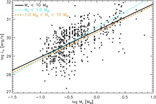
X-ray luminosities as a function of stellar mass in the Orion nebular cluster obtained with the Chandra X-ray Telescope as part of the COUP project (Preibisch et al. 2005).
It is worth noticing at this point that the slopes quoted include the entire sample of accretors and non-accretors in the Preibisch et al. (2005) data set. According to Preibisch et al. (2005), however, there are differences in the X-ray luminosities between accretors and non-accretors, where non-accretors show marginally higher X-ray luminosities that are roughly consistent with those of rapidly rotating main-sequence stars and they also show a clearer correlation with stellar mass, compared to the accretors. The accretors, on the other hand, have somewhat suppressed X-ray luminosities and the correlation with stellar mass is also not so clear; this is probably due to whatever effect is suppressing the X-ray luminosity, which may have to do with the presence of a disc or with whatever is damping the X-ray activity (although see Drake et al. 2009 for the opposite interpretation). One has to be careful however not to overinterpret this discrepancy and it is indeed difficult to estimate any uncertainty on the X-ray luminosity function. The main problem is that the definition of accretors and non-accretors used by Preibisch et al. (2005) was based on emission lines and it is well known that these can show strong time variability, leading to large uncertainties in the classification. In view of this, and also considering the differences between this data set and the Taurus data set which will be discussed below, we conclude that the uncertainties on the quoted value of the slope in the X-ray luminosity function are probably larger than those stated here.
Fig. 3 shows the same for the sample of Güdel et al. (2007) obtained with the XMM–Newton X-ray telescope in the Taurus molecular cloud. The number of sources in this survey is however much lower and hence it is more difficult to draw significant statistics, particularly in the higher mass bin. However, qualitatively similar results are obtained, where β = 1.38, 1.44 and 1.04 for the whole sample, the lower and the higher mass ranges defined above, respectively.
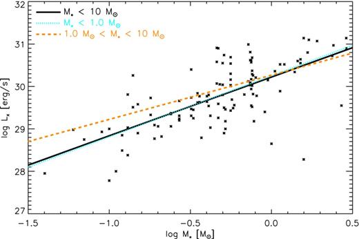
X-ray luminosities as a function of stellar mass in the Taurus molecular cloud obtained with the XMM–Newton X-ray telescope (Güdel et al. 2007).
The values of β obtained for the lower mass objects in the Preibisch et al. (2005) sample compare well with the values of α obtained for the same mass range, which is what one would expect if disc dispersal in this stellar mass range is dominated by X-ray photoevaporation. The same process is not expected to be the dominant disc dispersal mechanism for discs around high-mass stars, where X-ray production is expected to be lower and the corresponding photoevaporation rates are then too weak to compete with the higher accretion rates. In this context, the lack of agreement between α and β in the higher mass range is not surprising. It is difficult to speculate what the dominant dispersal mechanism at higher masses may be. The drop in the X-ray luminosities for these higher mass stars, implies that if photoevaporation is still the main driver of dispersal, the main heating source must be EUV or far-ultraviolet (FUV) photons. Detailed hydrodynamical wind solutions for these objects have yet to be calculated, although some estimates using a simpler approach were provided by Gorti, Dullemond & Hollenbach (2009), which show that photoevaporation by FUV radiation may be a viable solution for the fast dispersal of discs around higher mass stars.
If X-ray photoevaporation is indeed controlling disc dispersal around low-mass stars, hence determining the slope of the |$\skew3\dot{M}{\rm -}M_*$| relation, one other issue to be considered is the lowest possible accretion rate measurable at a given mass in a sample of discs that are dispersed by X-ray photoevaporation. Owen et al. (2010) show that the final phase of rapid disc dispersal begins roughly when the accretion rates become about a factor of 10 lower than the photoevaporation rates. For the ONC sources shown in Fig. 1, the lowest X-ray luminosities for solar mass stars are of the order of approximately 1029 erg s−1. This corresponds roughly to X-ray photoevaporation rates of 10−9 Mȯ yr−1, implying that the lowest accretion rates that should be measurable are of the order of 10−10 Mȯ yr−1, which is consistent with observational data in this mass bin (M12).
A final, perhaps more stringent test of this model is a comparison of the LX-M* distribution against the |$\skew3\dot{M}{\rm -}M_*$| distribution. The one-to-one mapping of the wind mass-loss rate with the X-ray luminosity would indeed suggest that their normalized distribution in the low-mass bin, where X-ray photoevaporation dominates, should be indistinguishable. Unfortunately, a direct comparison of the data sets is impossible since the distributions of stellar masses in the two samples (even in bins around solar-type stars) is formally different to very high significance. The likely cause of this is that our |$\skew3\dot{M}{\rm -}M_*$| sample contains a large number of objects from Taurus, which is known to have an unusual initial mass function (IMF; Luhman 2004). Therefore, in order to perform a meaningful statistical test we need to resample both distributions on to the same underlying mass function.
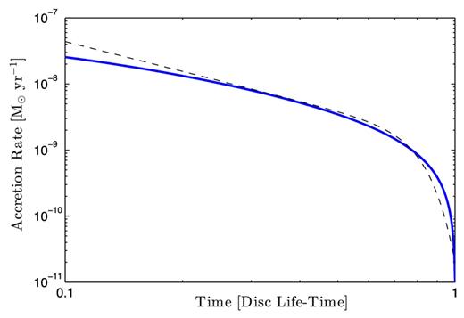
Comparison between a full viscous calculation (solid) and the simple formula (dashed).
Such a formula provides an approximate description of the disc's accretion rate evolution. The |$\skew3\dot{M}{\rm -}L_{\rm X}$| distribution is thus convolved with this expression in order to produce an |$\skew3\dot{M}{\rm -}M_*$| relation which can then be compared with the observed |$\skew3\dot{M}{\rm -}M_*$| relation. Thus, with our two resampled |$\skew3\dot{M}{\rm -}M_*$| relations (one observed and one calculated from M*-LX), we calculated the Kaplan–Meier distributions and perform a null-hypothesis test to determine whether we can reject the null hypothesis that these two distributions are different. Since we are resampling our two distributions on to the same underlying mass distribution we perform 500 realizations of this random samplings to get a sense of the resampling error. In Fig. 5, we show the Kaplan-Meier distributions resulting from 10 resampling realizations for the observed |$M_*{\rm -}\skew3\dot{M}$| (solid) and the |$M_*{\rm -}\skew3\dot{M}$| distributions calculated from the observed M*-LX distribution (dashed). Furthermore, in Fig. 6 we show a histogram of the P values resulting from our hypothesis tests (both using the log rank and Gehan methods – see Feigelson & Nelson 1985) for each of our random realizations, where the P value is an estimate of the probability that the two distributions are drawn from the same underlying sample. Therefore, they are unlikely to come from the same underlying distribution if P is small (<0.05 ∼2σ). Given that in our case P is clearly generally not small, so one cannot rule out the null hypothesis. This is striking given that the two distributions should be independent unless they are connected by the photoevaporation model. In summary, both figures show extremely good agreement between the two distributions and we are unable to reject the null hypothesis, suggesting that the two populations are indeed connected by the X-ray photoevaporation model.
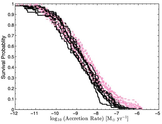
KM distributions for the resampled |$\skew3\dot{M}{\rm -}M_*$| (solid) and calculated |$\skew3\dot{M}{\rm -}M_*$| (dashed) relations.
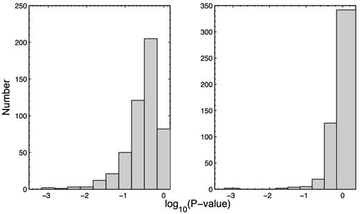
P values from the hypothesis test: log rank (left), Gehan (right).
We note, further, that the disagreement is very small, and mostly evident at high accretion rates which are likely dominated by accretion rates calculated from flaring X-ray values. Furthermore, the simple viscous model is likely to break down at early times due to variability.
The X-ray luminosity data then show, in summary, that the observed |$\skew3\dot{M}{\rm -}M_*$| relation in pre-main-sequence stars is consistent with being a simple consequence of disc dispersal by X-ray photoevaporation.
4 SUMMARY
We have presented a statistical analysis of accretion rates of pre-main-sequence stars as a function of stellar mass in order to establish whether the steep relation between accretion rates and mass may be a consequence of selection or detection thresholds, as feared in past (e.g. CP06; Tilling et al. 2008). With the large amount of data available we show (using survival statistics) that selections/detection biases are not driving the |$\skew3\dot{M}{\rm -}M_*$| relation.
We find the slope of the power-law relation to be between ∼1.6 and 1.9 for stars with masses lower that 1 Mȯ. Such slopes are similar to the slopes observed in the X-ray luminosity function of young stars in near-by clusters (e.g. Preibisch et al. 2005; Güdel et al. 2007). We show that X-ray photoevaporation predicts indeed that the observed |$\skew3\dot{M}{\rm -}M_*$| relation should be completely determined by the X-ray luminosity of the stars, which thus imprints a signature on the observed accretion rates distribution in a given cluster.
Furthermore, we demonstrate that a synthetic |$\skew3\dot{M}{\rm -}M_*$| data set constructed from the X-ray luminosity function of young stars in the Orion nebular cluster (Preibisch et al. 2005) is statistically indistinguishable from the observed |$\skew3\dot{M}{\rm -}M_*$| data set, hence lending further support that discs around young stars disperse predominantly by X-ray photoevaporation.
ACKNOWLEDGEMENTS
We thank the anonymous referee for a positive and constructive report. The calculations were partially performed on the Sunnyvale cluster at CITA which is funded by the Canada Foundation for Innovation.
Note that the form of the accretion rate evolution looks very similar to the semi-analytic solutions presented by Ruden (2004) using a Green's function approach for the EUV wind.
