


Abstract
The near-Earth asteroid belt is continuously replenished with material originally moving in Amor-class orbits. Here, the orbit of the dynamically interesting Amor-class asteroid 2012 XH16 is analysed. This asteroid was discovered with the Vatican Advanced Technology Telescope (VATT) at the Mt Graham International Observatory as part of an ongoing asteroid survey focused on astrometry and photometry. The orbit of the asteroid was computed using 66 observations (57 obtained with VATT and 9 from the Lunar and Planetary Laboratory-Spacewatch II project) to give a = 1.63 au, e = 0.36, i = 3| $_{.}^{\circ}$|76. The absolute magnitude of the asteroid is 22.3 which translates into a diameter in the range 104–231 m, assuming the average albedos of S-type and C-type asteroids, respectively. We have used the current orbit to study the future dynamical evolution of the asteroid under the perturbations of the planets and the Moon, relativistic effects, and the Yarkovsky force. Asteroid 2012 XH16 is locked close to the strong 1:2 mean motion resonance with the Earth. The object shows stable evolution and could survive in near-resonance for a relatively long period of time despite experiencing frequent close encounters with Mars. Moreover, results of our computations show that the asteroid 2012 XH16 can survive in the Amor region at most for about 200–400 Myr. The evolution is highly chaotic with a characteristic Lyapunov time of 245 yr. Jupiter is the main perturber but the effects of Saturn, Mars and the Earth–Moon system are also important. In particular, secular resonances with Saturn are significant.
INTRODUCTION
One of the research projects currently pursued at the Vatican Observatory is a study of the near-Earth object (NEO) population focusing on astrometry and photometry.
Observing programmes make use of the Vatican Advanced Technology Telescope (VATT), which includes the 1.8-m Alice P. Lennon telescope, to search for new asteroids and target known main-belt asteroids, Centaurs and trans-Neptunian objects (TNO). The telescope is located at the Mt Graham International Observatory, and it started operation in 2000 December to 2001 May acquiring CCD images at the primary focus, f/1.0 (Hergenrother & Spahr 2001). The first ‘new’ asteroid discovered with the VATT was found in 2000: (220696) = 2004 RA316 = 1999 TF241 = 2000 YJ143 by W. H. Ryan. During the years 2000–2005, Ryan and his assistants discovered about 60 new asteroids. In 2007, 75 new asteroids were discovered by C. W. Hergenrother.
A new observational programme for the search and observations of asteroids was started in 2009 by R. P. Boyle and K. Cernis. The first object observed was an asteroid of the Centaur group, 2009 HW77 (Cernis & Eglitis 2009), discovered in 2009 April. This interesting asteroid was observed with the VATT in three oppositions (2010–2012), and its new orbit was calculated by Wlodarczyk, Cernis & Eglitis (2011). Since 2010, imaging is performed at the Gregorian focus using a 4k background-illuminated CCD camera with liquid nitrogen cooling. With this 62 × 62 mm (2000 × 2000 binned pixels) camera, the field of view is 13 arcmin × 13 arcmin, with a scale of 0.38 arcsec pixel−1. All astrometric measurements are done using the astrometrica software developed by H. Raab.1 The catalogues USNO-A2.0, USNO-B1.0, UCAC-4 and others serve for the selection of reference stars in the astrometrica software. The limiting magnitude for stars on the VATT telescope is about R = 22.5 mag on unfiltered CCD images with an exposure time of about 360 s and a 1 arcsec seeing. It is a very useful instrument for follow-up astrometry of poorly observed NEOs, faint unusual objects and comets. The targets for observations are selected using public web tools for observers (IAU MPEC or ‘The NEO Confirmation Page’). About 2000 CCD images have been obtained to perform astrometry of asteroids and comets during the last four years. The methodology used to process CCD images and search for asteroids is similar to the one used in our earlier papers (Cernis et al. 2008, 2010).
In 2010–2013, during a sky survey of the ecliptic regions and follow-up astrometry of asteroids, 85 new asteroids were designated by the Minor Planet Center (MPC). Among them, 10 are multiple-apparition objects, 19 are one-opposition objects and 64 are one-opposition objects with low-accuracy orbits. For six objects, high-precision orbits have been determined. Among the discovered asteroids and in addition to 2012 XH16, there is one TNO 2012 BX85 (Cernis & Boyle 2012) and two Centaur-class asteroids: 2012 DS85 and 2012 VU85 (Cernis et al. 2012b). The orbit of the asteroid 2012 XH16 is dynamically interesting due to resonances affecting it, caused by planetary perturbations, that may lead 2012 XH16 to evolve from the Amor asteroid category to near-Earth belt membership (Bottke et al. 1996).
To investigate the behaviour of the orbit we used two free software packages: the orbfit2 and the software of M. Broz (modified swift-rmvsy3). The orbfit software has been used to process the astrometry and the swift-rmvsy package has been used to compute the dynamical evolution. The package developed by Broz is a modified version of the widely used swift package (Levison & Duncan 1994).
In Section 3, we describe the method of selection and weighting of the observational material and the catalogue biased method used to improve the orbit of asteroid 2012 XH16. These methods are used in orbital computations of asteroids by the NEODyS4 and the NASA's JPL.5 In Section 3.1, we study the orbital evolution of asteroid 2012 XH16 between the years 3000 bc to ad 3000 and searched for close approaches (CAs) with the planets and the Moon. The multiplicity of CAs leads to the chaotic evolution of the orbit of asteroid 2012 XH16. In this section, we also present time evolution of the asteroid 2006 WB30. We present the results of recalculating the orbital evolution without: the Earth–Moon system, Mars, Jupiter and Saturn together with the results including all the planets. In Figs 4 and 7, the influence of the Jupiter is visible. In Section 4, we compute the influence of the Yarkovsky effect on the motion of 2012 XH16 using the M. Broz's software. The physical parameters of 2012 XH16 are poorly known and, as a result, we take some of them as randomly chosen values in our calculations. In Section 5, we find a Lyapunov time of 245 yr for the orbit of 2012 XH16, which is the result of the very chaotic nature of the motion of this object.
In Section 6, we analyse the secular orbital resonances of the asteroid 2012 XH16 using the orbfit software. This service is available from the AstDyS portal6 and provides a graphical tool to access information on the proper elements of known asteroids and also data on their stability, asteroid families and resonances. Tools to help the possible recovery of lost asteroids are also given.7 Finally, in Section 7, we present ephemerides of the Amor-class asteroid 2012 XH16 for the one possible observational window in the next 50 yr.
DISCOVERY OF ASTEROID 2012 XH16
Asteroid 2012 XH16 was discovered on the early hours of 2012 December 5 (Cernis, Boyle & Laugalys 2012a) during a search for new asteroids with the VATT telescope and a CCD camera. The discovery time and position are listed in Table 1. During the inspection of our CCD frames, the asteroid was detected in six 300 s exposures as a fast moving object (motion from east to west at about 1.17 arcsec min−1) at solar elongation 169°, about 4° above the ecliptic plane in the constellation of Taurus (about 3° east of the open star cluster Messier 45, the Pleiades). The object was identified on December 5 by K. Cernis at about 15 h ut (7 h after it was imaged). The stacked discovery image is shown in Fig. 1. One night positions with a 0.5 h arc were reported to MPC. The object was put on the NEO Confirmation Page. K. Cernis made quick astrometric and photometric measurements of the new object to calculate its approximate position for the next night and also found an apparent magnitude R = 21.2 mag. In clear weather, we began searching for the new object by midnight December 6, about 0.5°west from the discovery position. After a few attempts, the object was found in 14 images by R. Boyle and V. Laugalys obtained on December 6.267. The discovery was further confirmed by our observatory the following night, on December 7.311 (11 images). On December 7, T. Spahr at MPC designated the new object as 2012 XH16 and calculated its first preliminary orbit with a period of 2.04 yr.
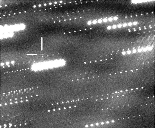
Discovery image of the Amor-class asteroid 2012 XH16. The size of the field is 2.7 arcsec × 3.3 arcsec. The image was stacked up using six images (6 × 300 s exposures) taken at the Mt Graham Observatory with the VATT on the night of 2012 December 5.
The discovery time and the astrometric position of the Amor-class asteroid 2012 XH16. The image was stacked up using six images (6 × 300 s exposures), with NEO object sky motion parameters 1.17 arcsec min−1 and PA 279| $_{.}^{\circ}$|1.
| UTC | RA | Dec. | R (mag) |
|---|---|---|---|
| 2012 Dec 5.322 | 03h58m48|$.\!\!^{{\rm s}}$|23 | +24°38′07|${^{\prime\prime}_{.}}$|3 | 21.2 |
| UTC | RA | Dec. | R (mag) |
|---|---|---|---|
| 2012 Dec 5.322 | 03h58m48|$.\!\!^{{\rm s}}$|23 | +24°38′07|${^{\prime\prime}_{.}}$|3 | 21.2 |
During seven nights, 57 astrometric positions were collected at the VATT Observatory. The accuracy of the astrometric observations is about ±0.13 arcsec with a signal-to-noise ratioof about 5 in the 6 min exposure images. The asteroid has also been observed by the 1.8-m telescope of the Spacewatch II programme at Kitt-Peak observatory during two nights in 2013 January and February (McMillan, Bressi & Scotti 2013a; McMillan et al. 2013b).
A total of 66 astrometric points were collected, of which 86 per cent belong to the VATT Observatory where the asteroid was observed from 2012 December 5 until 2013 April 15. Then, in 2013 May 3–13 additional observations of the area of the sky where the asteroid was expected to be were obtained during three nights; however, 2012 XH16 was not detected due to its faintness. Asteroid was supposed to be between magnitude 22.1 V (May 3) and 22.4 V (May 13) and the limiting magnitude of the CCD frames those nights was about 21.9 V–22.1V.
Table 2 lists the computed orbit of the asteroid 2012 XH16 published by the MPC in M.P.O. 260829.8 Table 2 presents orbital elements: a – semimajor axis, e – eccentricity, i – inclination, Ω – longitude of the ascending node, ω – argument of perihelion and M – mean anomaly. The orbit was computed from 65 astrometric positions. One observation was rejected as an outlier. Table 2 also includes the current orbital elements as posted by the MPC, the JPL Small-Body Database and the NEODyS-2.
The keplerian orbital elements of asteroid 2012 XH16 from different current sources.
| a (au) | e | i (°) | Ω (°) | ω (°) | M (°) |
|---|---|---|---|---|---|
| Epoch 2013 Nov. 04.0 = JDT 245 6600.5 | |||||
| JPL Small-Body Database | |||||
| 1.631 6098 | 0.360 4865 | 3.757 19 | 53.006 95 | 100.526 18 | 113.578 68 |
| ±4.28e−05 | ±1.53e−05 | ±0.000 11 | ±0.000 23 | ±0.000 38 | ±0.004 52 |
| NEODyS-2 | |||||
| 1.631 6097 | 0.360 4865 | 3.757 19 | 53.006 96 | 100.526 18 | 113.578 68 |
| ±4.38e−05 | ±1.57e−05 | ±0.000 11 | ±0.000 23 | ±0.000 39 | ±0.004 63 |
| Epoch 2013 Apr. 18.0 = JDT 245 6400.5 | |||||
| M.P.O. 260 829 | |||||
| 1.631 4437 | 0.360 4231 | 3.757 37 | 53.008 99 | 100.512 33 | 19.007 77 |
| MPC | |||||
| 1.631 4437 | 0.360 4231 | 3.757 37 | 53.008 99 | 100.512 33 | 19.007 77 |
Fig. 2 plots the orbit of the near-Earth asteroid 2012 XH16 and the planets: Mercury, Venus, Earth and Mars. The positions of the planets are referred to the epoch of discovery and are marked by the different symbols, asteroid 2012 XH16 is marked by the star. As seen in Fig. 2, the orbit of asteroid 2012 XH16 crosses the orbit of Mars and the nodal points are very close to the intersection, making very close flybys possible.
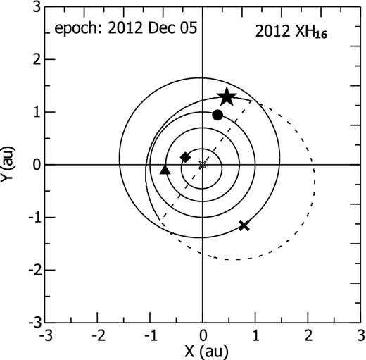
The orbit of 2012 XH16 in the ecliptic plane. Positions of the asteroid and planets are presented for the date of discovery, 2012-12-05 = JD 245 6266.5. The dashed line denotes the part of the orbit below the ecliptic plane.
ORBIT OF ASTEROID 2012 XH16
Currently, 2013 November 6, there are 10 313 near-Earth asteroids (q < 1.3 au): 810 Atens with orbits similar to that of 2062 Aten (a < 1.0 au; Q > 0.983 au), 5125 Apollos with orbits crossing the Earth's orbit similar to that of 1862 Apollo (a > 1.0 au; q < 1.017 au) and 4378 Amors with orbits similar to that of 1221 Amor (1.017 au < q < 1.3 au). They are listed at the MPC9 and at the JPL NASA.10
The MPC and the JPL NASA classified asteroid 2012 XH16 as an Amor-class object. The Minor Planet Ephemeris Service gives the orbit of the asteroid 2012 XH16 based on 65 optical observations together with the residuals.11
But when we observe asteroids, it is necessary to know the actual orbit of the asteroid, with the last available observations, to compute ephemerides for the next observational window. To compute the orbit of the asteroid and ephemerides for different dynamical cases, we used the freely available orbfit software v.4.2.12 This new version includes the new error model based on Chesley, Baer & Monet (2010).
In all of our computations, we follow the same method in the weighting and selection of observations that is being used by the NEODyS site. For each measured right ascension and declination the a priori rms was used. They are computed based on the statistical performance of the given observatory. The NEODyS site keeps a summary of these statistics for each observatory. The VATT statistics are also available from the NEODyS site list.13 If insufficient observations are available for statistical analysis, then the NEODyS site uses an a priori rms of 3 arcsec for observations obtained before 1890, 2 arcsec for those acquired prior to 1950 and 1 arcsec for those obtained afterwards. For automatic rejection of bad observations, the value of χ from the usual χ2 test is provided. This parameter gives a characterization of the relative quality of the observation for a given asteroid. Next automatic outlier rejection routine discards observations at |$\chi = \sqrt{10}$| and recovers at |$\chi = \sqrt{9.21}$|. It should correspond to 1 per cent of rejections if the errors are close to Gaussian.
For all observations, the residuals, both in right ascension and declination, and the parameter χ are computed by the NEODyS site or by us using the orbfit software.
For H = 22.29, and an albedo of 0.20 for S-type and 0.04 for C-type asteroids, we find the diameter of 2012 XH16 to be between 104 and 231 m, respectively. The JPL NASA lists H = 22.286 and the NEODyS, 22.3 with 100 < D < 230 (m), respectively. The NEODyS size range has been derived from H, considering the limiting cases of the albedos of C- and S-types, 0.04 and 0.20, respectively.
All orbital elements given in Table 3 were computed using the JPL Planetary and Lunar Ephemerides DE405 and the relativistic effects. The 2012 XH16 orbit computations have been performed using initial conditions (positions and velocities in the barycentre of the Solar system) provided by the JPL HORIZONS system (Giorgini et al. 1996; Standish 1998) and referred to the JDT 245 6600.5 epoch which is the t = 0 instant.
The orbit of 2012 XH16 calculated with the orbfit software with the 1σ errors (rms) of the parameters using catalogue biased model – top three lines, and without this model – next three lines.
| Epoch 2013 Nov. 04.0 TT = JDT 245 6600.5 | |||||
|---|---|---|---|---|---|
| a(au) | e | i(°) | Ω(°) | ω(°) | M(°) |
| The NEODyS weighting method | |||||
| Catalogue biased model | |||||
| 1.631 61 | 0.360 487 | 3.7572 | 53.0070 | 100.5262 | 113.5787 |
| ±0.000 04 | ±0.000 016 | ±0.0001 | ±0.0002 | ±0.0004 | ±0.0046 |
| rms = 0.6856 arcsec | |||||
| Without catalogue biased model | |||||
| 1.631 60 | 0.360 483 | 3.7572 | 53.0071 | 100.5262 | 113.5797 |
| ±0.000 05 | ±0.000 019 | ±0.0001 | ±0.0003 | ±0.0005 | ±0.0057 |
| rms = 0.4873 arcsec | |||||
The neodys and the orbfit software use star catalogue debiasing approach described in the previous paper. In the case of asteroid 2012 XH16, only biases for observations after 2012 December 13 are given.14 Table 3 presents a final orbit of the asteroid 2012 XH16 computed by us with the orbfit software using the catalogue biased model according to Chesley et al. (2010) and without this model. Additional perturbations from 16 massive asteroids were used with masses according to Farnocchia et al. (2013): (1) Ceres, (2) Pallas, (4) Vesta, (10) Hygiea, (3) Juno, (9) Metis, (15) Eunomia, (16) Psyche, (29) Amphitrite, (31) Euphrosyne, (52) Europa, (65) Cybele, (87) Sylvia, (511) Davida, (532) Herculina and (704) Interamnia. The observations of asteroid 2012 XH16 are not as precise as in the case of asteroid (99942) Apophis but we used the same gravitational model as Farnocchia et al. (2013) for all standard orbital computations.
Fig. 3 presents residuals in right ascension computed for unbiased and biased catalogue model for observations of 2012 XH16. The small role of catalogue biased model is visible.
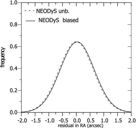
2012 XH16. Residuals in right ascension for the unbiased and biased catalogue model.
Time evolution of orbital elements of the Amor-class asteroid 2012 XH16
First, we compute the time evolution of the orbital elements of the nominal orbit using the mercury software package with the Everhart's RA15 (RADAU) integration method (Chambers 1999). Then, we analyse the effects of the perturbations resulting from the various planets on the dynamics of 2012 XH16. The purpose of these new calculations is to disentangle the dynamical role of the various planets. In order to do that, we use the best nominal orbit calculated with the catalogue biased model from Table 3 and compute the time evolution of the orbital elements of asteroid 2012 XH16 for 10 000 yr backwards and forward.
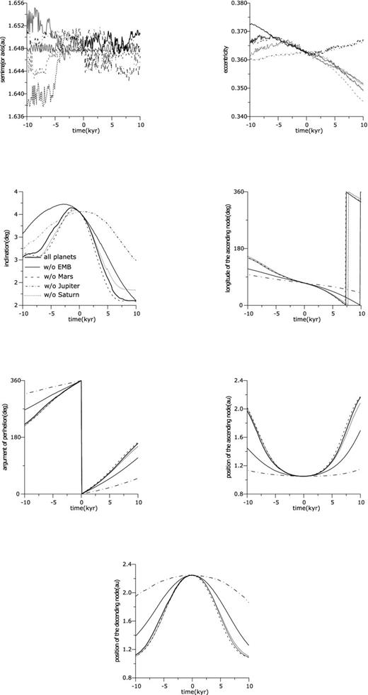
Fig. 4 presents the results of recalculating the orbital evolution without: the Earth–Moon system, Mars, Jupiter and Saturn together with the results including all the planets. Orbital elements are plotted every 100 yr from the starting epoch of the orbital elements of the asteroid 2012 XH16, t0 = 2456 600.5 = 2013-Nov-04.0.
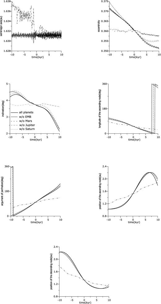
Time evolution of the nominal orbit of the asteroid 2012 XH16 10 000 yr backwards and forward from the osculating epoch 2013-Nov-04.0. Continuous thick line presents time evolution with all planets, thin line – without the Earth–Moon system, dashed line – without Mars, dashed and dotted line – without Jupiter and dotted line – without Saturn. Positions of the asteroid 2012 XH16 are marked every 100 yr.
It is clear that Jupiter significantly affects the subsequent orbital evolution. Excluding Saturn has noticeable effects mainly on the eccentricity after about 5000 yr into the future and into the past, and on the semimajor axis about 2000 yr into the past. Excluding Mars and the Earth–Moon system have only minor effects and they are smaller than those observed in the cases without Jupiter or Saturn.
Part of the semimajor axis drift can be connected with the Yarkovsky/YORP effects and will be studied in the next section.
To study the time evolution of the dynamically interesting asteroid 2012 XH16, it is not enough to follow the evolution of the nominal orbit; a swarm of ‘clones’ with orbital elements similar but compatible with the rms of the nominal orbit must also be studied. Therefore, we computed the time evolution of 2001 virtual asteroids (VAs) or ‘clones’ using the multiple solution method of Milani et al. (2005a,b) for the 5σ uncertainty around the nominal orbit of the asteroid 2012 XH16.
Then, we propagated these 2001 VAs forward to ad3000 and backwards to 3000 bc, using the orbfit software and the JPL DE406 Solar system model, i.e. about 1000 yr in the future and 5000 yr in the past from the starting date of integration 2013-Nov-04.0 (the osculating epoch of the orbital elements of the asteroid 2012 XH16 from Table 3.). These integrations show that there are many CAs of 2012 XH16 to the Earth–Moon system and Mars. As presented in Fig. 5, the CAs are much deeper than 0.02 au in the case of Mars, especially around 800 yr into the past. Only some CAs are found in the future.
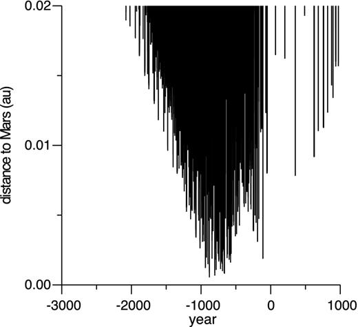
CAs of 2012 XH16 to Mars.
CAs of 2012 XH16 to Mars and the Earth.
| Years from | Distance | ||
|---|---|---|---|
| t0 = 2013 Nov. 04.0 | (au) | (radii of planet) | (rH) |
| Mars | |||
| Past | |||
| −879.541 | 0.000 89 | 39 | 0.136 |
| −879.540 | 0.000 54 | 24 | 0.082 |
| −879.539 | 0.000 93 | 40 | 0.142 |
| −802.245 | 0.000 66 | 29 | 0.101 |
| −802.424 | 0.000 85 | 37 | 0.129 |
| −691.453 | 0.000 98 | 43 | 0.149 |
| −667.001 | 0.000 84 | 37 | 0.128 |
| −663.239 | 0.000 81 | 35 | 0.123 |
| Future | |||
| 353.197 | 0.008 | 348 | 1.218 |
| rH = 0.006 570 au | |||
| Radius of Mars = 3396 km = 0.000 023 au | |||
| Earth | |||
| Past | |||
| −4997.877 | 0.047 60 | 1107 | 4.839 |
| −4987.880 | 0.049 59 | 1153 | 5.041 |
| −4835.881 | 0.049 73 | 1157 | 5.055 |
| Future | |||
| 849.356 | 0.080 00 | 1861 | 8.133 |
| 874.364 | 0.079 99 | 1860 | 8.132 |
| 947.359 | 0.079 80 | 1856 | 8.112 |
| 951.367 | 0.079 76 | 1855 | 8.108 |
| 972.357 | 0.079 77 | 1855 | 8.109 |
| 976.358 | 0.079 51 | 1849 | 8.083 |
| rH = 0.009 837 au | |||
| Radius of the Earth = 6378 km = 0.000 043 au | |||
Fig. 6 shows CAs of the asteroid 2012 XH16 to the Earth deeper than 0.1 au. We observe that these CAs are not as deep as those with Mars. Only at the end of the backward integrations, we found several CAs deeper than 0.05 au. Moreover, during the following 800 yr there are no CAs under 0.1 au.
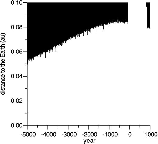
CAs of 2012 XH16 to the Earth.
Time evolution of the nominal orbit of the asteroid 2006 WB30 10 000 yr backwards and forward from the osculating epoch 2013-Nov-04.0. Designations are the same as in Fig. 4 for the asteroid 2012 XH16.
The accuracy of computations with the orbfit software during forward and backward integrations is described in Wlodarczyk (2008), and the use of the multiple solution method in Wlodarczyk (2009).
The time evolution of the orbit of the asteroid 2012 XH16 is similar to the asteroid 2006 WB30 (see Fig. 7). We computed that in the 10 000 yr forward integration semimajor axis of 2012 XH16 has almost the same value of about 1.63 au. Similarly, the semimajor axis of 2006 WB30 has almost the same value of about 1.65 au. Computations were made according to the swift integrator of M. Broz using all planets. However, it is worth noting that both asteroids orbit close to the 1:2 mean motion resonance with the Earth (1:2E) around 1.6 au. The orbital period of asteroid 2012 XH16 is nearly 761 d and that of 2006 WB30 is close to 773 d.
According to Gallardo (2006), the 1:2E resonance is strong and relatively isolated in the region between 1.5 and 2.0 au. Objects move in relatively stable orbits and could survive despite experiencing frequent close encounters with Mars. We have found almost the same dynamical behaviour for both asteroids, 2012 XH16 and 2006 WB30. There are some differences in the evolution of the positions of the ascending node and the descending node because of the differences in the starting values of the both nodes, but the range of their evolution changes are almost the same, between 1.0 and 2.2 au.
Asteroids 2012 XH16 and 2006 WB30 belongs to the Amor-class, i.e. its perihelion distance is between 1.0 and 1.3 au. For the asteroid 2012 XH16, we made additional 10 Myr integration backwards and forward. Results are shown in Fig. 8. The perihelion distance, q, of the nominal orbit changes its value from about 1.6 au 10 Myr into the past to about 1.05 au now and 1.3 au into the future 10 Myr.
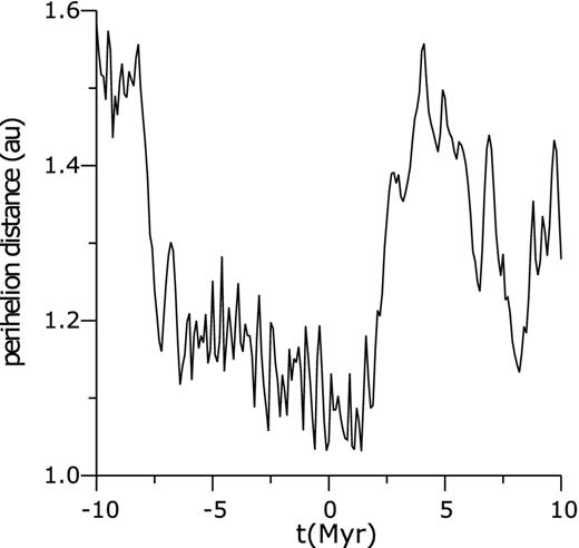
Time evolution of the perihelion distance of the asteroid 2012 XH16 during 10 Myr forward and backward integration.
INFLUENCE OF THE YARKOVSKY EFFECT ON THE MOTION OF ASTEROID 2012 XH16
The Yarkovsky and YORP (Yarkovsky–O'Keefe–Radzievskii–Paddack) effects are the result of thermal radiation forces and torques that cause a drift in the value of the semimajor axis of small asteroids and change their spin vectors. Both effects are described in detail by Bottke et al. (2006). The result of the Yarkovsky effect is the removal of small asteroids from the main belt into the chaotic mean motion and secular apsidal or nodal resonance zones. Then, their paths can be gradually transformed into Earth-crossing orbits. The Yarkovsky and YORP effects are now customarily included when studying the orbital evolution of objects crossing the Earth orbit (Milani et al. 2009; Kwiatkowski 2010; Kwiatkowski, Buckley & O'Donoghue 2010; Kwiatkowski, Polinska & Loaring 2010).
NEOs, like 2012 XH16, experience multiple close encounters with planets which change the values of its semimajor axis, eccentricity and inclination masking the Yarkovsky and YORP effects. To estimate the influence of the Yarkovsky and YORP effects on the motion of 2012 XH16, it is necessary to compute or estimate some input data: the temperature distribution on the surface and inside the asteroid among others. In order to do this, we need to know its orbit, size, shape and mass, orientation of spin axis and axial rotation period, density of surface layers, albedo, thermal conductivity, thermal capacity and infrared emissivity of the material. The physical parameters – bulk density, surface density, thermal conductivity, specific thermal capacity and mean albedo of ‘clones’ (VAs) were partially taken from Brŏz (2006) and they were assumed as shown in Table 5.
Typical values of the material thermal parameters for modelling the Yarkovsky and YORP effects used by Brŏz (2006) and assumed in this work for 2012 XH16, where ϱbulk denotes the bulk density, ϱsurf the surface density, K the thermal conductivity and C the specific thermal capacity.
| Material | ϱbulk | ϱsurf | K | C | Albedo |
|---|---|---|---|---|---|
| (kg m−3) | (kg m−3) | (W m−1 K−1) | (J kg−1 K−1) | ||
| Bare basalt | 3500 | – | 0.5–2.5 | 680 | 0.1–0.16 |
| Regolith | 3500 | 1500 | 0.001–0.01 | 680 | – |
| Metal | 8000 | – | 40 | 500 | 0.09–0.11 |
| C-type | 1000 | – | 0.1–1.0 | 1500 | 0.03–0.08 |
| 2012 XH16 | |||||
| th2: | 2500 | 2000 | 1.0/0.01 | 680 | 0.38 |
| th2a: | 3500 | 3000 | 1.0/0.01 | 680 | 0.38 |
| th3: | 2500 | 2000 | 1.0/0.01 | 1500 | 0.38 |
| th3a: | 3500 | 3000 | 1.0/0.01 | 1500 | 0.38 |
| th4: | 2500 | 2000 | 10/0.1 | 680 | 0.38 |
| th4a: | 3500 | 3000 | 10/0.1 | 680 | 0.38 |
In Brŏz (2006), the rotational period of asteroids is computed using the assumption that they have a diameter of 1 km, i.e. with radius R = 500 m, has the rotational period T = 5 h. Generally, for asteroids of radius R(m), the rotational period is given by T(h) = 5 × (2R/1000). The value of the diameter of the asteroid 2012 XH16 computed in Section 3 is in the range 104–231 m. Hence, the mean value of the diameter of the asteroid 2012 XH16 is about 168 m and the estimated rotational period, given by the T approximation, is equal to 0.84 h.
To study the influence of the Yarkovsky effect on the motion of the asteroid 2012 XH16, we computed propagation of the orbital elements of the asteroid 2012 XH16 with and without the Yarkovsky effect.
As we mentioned above, in order to compute the Yarkovsky and YORP effects, it is necessary to know the orientation of the spin axis of the asteroid. This parameter is unknown and therefore we took it as a random value. The values of the azimuth and the height of the spin axes in the ecliptical reference frame were chosen from the interval (0, 360)° and (−90,+90)°, respectively. It was assumed that the infrared emissivity is equal to 0.60 for all VAs.
First, we computed the time evolution of the nominal orbit into the next 10 000 yr with and without the Yarkovsky effect. As starting orbit, we take the best nominal orbit computed with the catalogue biased model from Table 3. Next, we assumed some physical parameters as pointed out above (see Table 5) for asteroid 2012 XH16 to compute the time evolution of its nominal orbit. We take into account modified physical parameters from case th2 in Table 5, i.e. bulk density 2500 kg m−3, surface density 2000 kg m−3, thermal conductivity 0.01 W m−1 K−1, specific thermal conductivity 680 J kg−1 K−1 and albedo 0.38. As diameter of the asteroid 2012 XH16, we take its average value computed by us, i.e. 168 m. Additionally, we computed the time evolution for different values of the adopted spin of 2012 XH16. In the ecliptic reference frame, we used a fixed value of 0° for the azimuth of the spin and changed only its height. Hence, for different values of spin (its height) we got differences in the values of the orbital elements of the nominal orbit of the asteroid 2012 XH16 computed with and without the Yarkovsky effect in the next 10 000 yr.
In all cases presented in equations (5)–(8), the semimajor axis drift, connected with the Yarkovsky/YORP effect only, is smaller than the average semimajor axis drift of the asteroid 2012 XH16 of about −2.70 × 10⁻⁴ au, see equation (2). Using other possible physical parameters of the asteroid 2012 XH16 from Table 5 we can get different values of the semimajor drift but the contribution of the Yarkovsky effect should be smaller than other effects, for example planetary perturbations, as showed in Fig. 4 and the chaotic motion due to the CAs to Mars and the Earth–Moon system.
Fig. 9 and equations (5)–(8) present only quantitative results of the influence of the Yarkovsky/YORP effect on the motion of the asteroid 2012 XH16 in the nominal orbit. Using the mentioned multiple solution method, we computed 11 VAs of the asteroid 2012 XH16 with the 1σ uncertainties in the orbital elements. Then each of the VA was propagated 10 000 yr in the future using the same procedure as for the nominal orbit with the results presented in the Fig. 9. Each of the VA has the same physical parameter and the spin like the asteroid in the nominal orbit. They only differ by the starting orbital elements connected with the construction of the VAs, i.e. using the multiple solution method. It was appeared that the differences in the values of the orbital elements of the different VAs of the asteroid 2012 XH16 computed with and without the Yarkovsky effect depend on the given VA. Only VAs close to the nominal orbit have almost the same value of the parameter da/dt like the asteroid in the nominal orbit. This behaviour is connected with the chaotic motion of the asteroid 2012 XH16 as will be shown in the next section.
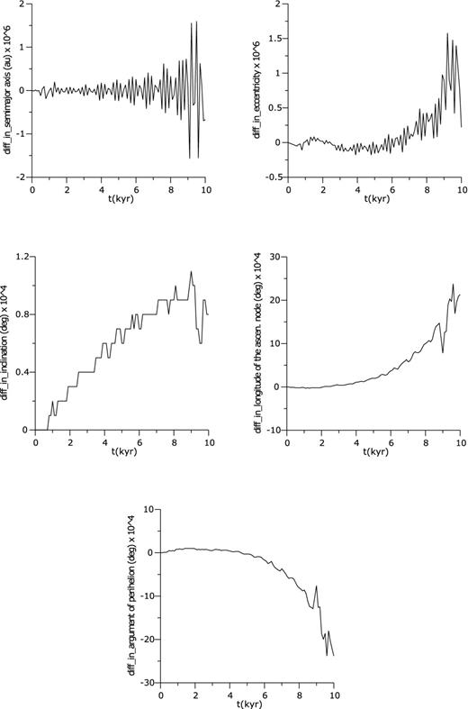
Differences in the values of the orbital elements of the nominal orbit of the asteroid 2012 XH16 computed with and without the Yarkovsky effect in the 10 000 yr in the future. Hence, da(au) = −1.793 × 10− 9 × t(kyr) + 2.725 × 10− 9.
Next, we computed the starting orbital elements of 101 VAs with the orbfit software by applying the multiple solution procedure described in Milani et al. (2005a,b) and considering 3σ errors. Then, the orbital elements were added as input files to the swift software (Brŏz 2006). This software allows us to compute the evolution of orbital elements of clones without and with the Yarkovsky and YORP effects.
The asteroid experiences multiple close encounters with Mars and more distant flybys with the Earth–Moon system as presented in Table 4 and Figs 5 and 6. As a result, even small changes in the position of the asteroid in phase space can lead to different dynamical behaviour in the future (Wlodarczyk 2007).
Hence, the asteroid 2012 XH16 has a very chaotic motion, as we discuss in detail in Section 5, and the dynamical evolution of all VAs depends mainly on changes in the semimajor axis, eccentricity and inclination caused by close planetary approaches. Moreover, close encounters with Mars are only possible near the nodes and the precession of the nodes depends on the semimajor axis, the eccentricity and the argument of perihelion. The influence of the Yarkovsky/YORP effects is difficult to separate from chaotic motion of the asteroid 2012 XH16. Different physical models of 2012 XH16 lead to different and unpredictable behaviour and their results are not very different from those obtained in the purely gravitational case. We can draw this from Table 6 where we present results of the 1 Gyr forward integration with and without the Yarkovsky/YORP effect using different physical models of asteroid 2012 XH16. Here ‘th’ refers to parameters in Table 5, ‘Out’ – number of VAs ejected from the Solar system (semimajor axis, a >100 au), ‘Sun’ – number of VAs which hit the Sun (perihelion distance, q < 0.004 68 au), ‘Mercury, Venus, Earth, Mars’ – number of VAs which hit given planet and ‘Time’ – time, in Myr, when in our Solar system model there are only Sun and planets without any VA of the asteroid 2012 XH16. All VAs are ejected from integration before 1 Gyr despite of the Solar system model. Hence, VAs of the asteroid 2012 XH16 can survive in the Amor region for about 200–400 Myr.
Behaviour of the VAs during a 1 Gyr forward integration.
| With Yarkovsky effect | W/O Yarkovsky effect | ||||||
|---|---|---|---|---|---|---|---|
| th2 | th3 | th4 | th2a | th3a | th4a | ||
| Out | 13 | 11 | 11 | 16 | 24 | 16 | 18 |
| Sun | 46 | 44 | 32 | 32 | 27 | 38 | 36 |
| Mercury | 3 | 3 | 0 | 5 | 4 | 3 | 2 |
| Venus | 9 | 11 | 11 | 7 | 8 | 9 | 11 |
| Earth | 3 | 6 | 6 | 6 | 8 | 10 | 4 |
| Mars | 0 | 0 | 0 | 1 | 1 | 1 | 0 |
| Time(Myr) | 244 | 380 | 387 | 227 | 376 | 190 | 343 |
LYAPUNOV TIME OF THE ASTEROID 2012 XH16
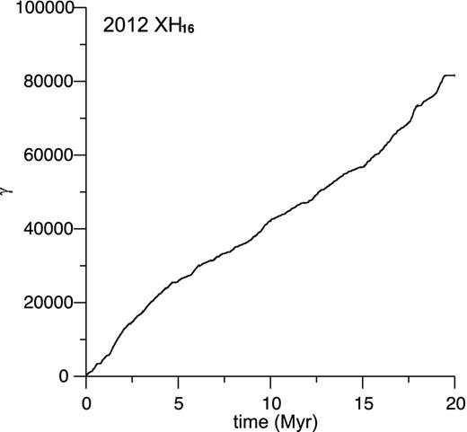
The time evolution of γ shows a smooth variation. The orbit of 2012 XH16 is chaotic with a Lyapunov time of about 245 yr.
SECULAR ORBITAL RESONANCES OF THE ASTEROID 2012 XH16
From the NEODyS data set,15 we can take the computed values of proper elements for the NEOs, i.e. the precession rate g of perihelion (the frequency of perihelion), which is equal to the sum of changes in the argument of perihelion, ω, and in the longitude of the ascending node, Ω, of the orbit of the asteroid, expressed in arcseconds per year and the precession rate s of the ascending node (the frequency of the ascending node), which is equal to the change in the longitude of the ascending node, Ω, of the orbit of the asteroid, expressed in arcseconds per year. Using the orbfit software with the implemented orbit9 software, we computed values of g and s for the orbit of asteroid 2012 XH16 [g = 20.4374(arcsec yr−1), s = −34.9866(arcsec yr−1)]. These values are consistent with those provided by the NEODyS data site.
A secular resonance occurs when the frequency of time-variation of the longitude of perihelion, g, or the longitude of the ascending node, s, of an asteroid becomes nearly equal to the orbital frequency of a planet (or is related to the combination of orbital frequencies of more than one planet). According to Milani & Knezevic (1994): A zk resonance is a resonant combination of the form k(g − g6) + s − s6, where k is integer, g and s, g6 and s6 denote the frequency of the longitude of perihelion and the frequency of the longitude of the ascending node of the asteroid and of Saturn [g6 = 28.2455(arcsec yr−1), s6 = −26.3450(arcsec yr−1)].
Fig. 11 presents the plane of proper frequency g of the longitude of perihelion versus proper frequency s of longitude of the ascending node for 10 029 near-Earth asteroids computed by the NEODyS as for 2013 November 10. Lines indicate the position of the z1, z2 and z3 secular resonances. The frequencies g and s shown in Fig. 11 are calculated according to the synthetic theory developed in Knezevic & Milani (2000). We computed them analytically using algorithm orbit version 9 as published in the NEODyS site. Fig. 11 shows that almost all the NEOs are inside the z1, z2 and z3 resonances. Resonance z3 bounds the population of almost all known NEOs.
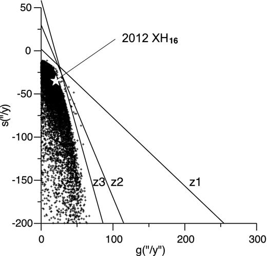
The plane of proper frequency g of the longitude of perihelion versus proper frequency s of longitude of the ascending node for 10 029 near-Earth asteroids. Lines indicate the positions of the zk secular resonances. Position of the asteroid 2012 XH16 is marked by a star.
PLANNING THE RECOVERY OF 2012 XH16 in 2036
During the next 50 yr, there is only one favourable observational window in which asteroid 2012 XH16 will be brighter than 22 mag. Table 7 lists dates of observation, astrometric positions in the sky (right ascension and declination), solar elongation of the asteroid (the angle Sun–observer–asteroid), the distance Sun–asteroid (R), the distance Earth–object (Delta), the sky plane error with the long axis (short axis is almost 0°) and the position angle of the sky plane error axis. The sky plane error is about 1° and the asteroid 2012 XH16 can easily be recovered using relatively small telescopes, i.e. about 2–3 m in diameter. We provide a longer table with weekly entries in order to facilitate a possible recovery. Almost the same ephemerides prediction results we can get from the NEODyS site16 and the NASA's JPL HORIZONS system.17 The ephemerides provided by the Minor Planet Ephemeris Service18 differs only by about 1 arcmin in RA and Dec. and lie in our computed 1σ uncertainty region. We hope that the Amor-class asteroid 2012 XH16 will be recovered in 2036 or perhaps earlier.
Ephemerides of the asteroid 2012 XH16 for its visibility window in 2035 and 2036. The coordinates (J2000) are for a geocentric observer.
| Date | RA | Dec. | m | Sol. | R | Delta | Sky | PA |
|---|---|---|---|---|---|---|---|---|
| Elo. | plane | |||||||
| error | ||||||||
| h m s | (°) (arcmin) | (°) | (au) | (au) | (arcmin) | (°) | ||
| 2035 | ||||||||
| 3 Dec | 09 03 57 | +23 22.1 | 22.6 | 118.3 | 1.24 | 0.42 | 42 | 107 |
| 10 Dec | 09 33 56 | +22 46.2 | 22.3 | 118.5 | 1.21 | 0.37 | 47 | 111 |
| 17 Dec | 10 06 59 | +21 50.5 | 22.0 | 117.9 | 1.18 | 0.33 | 52 | 115 |
| 24 Dec | 10 43 13 | +20 28.0 | 21.8 | 116.4 | 1.15 | 0.30 | 56 | 119 |
| 31 Dec | 11 22 12 | +18 32.4 | 21.7 | 114.0 | 1.12 | 0.27 | 59 | 124 |
| 2036 | ||||||||
| 7 Jan | 12 03 01 | +16 00.5 | 21.6 | 110.8 | 1.10 | 0.25 | 60 | 129 |
| 14 Jan | 12 44 17 | +12 55.3 | 21.5 | 107.2 | 1.08 | 0.24 | 59 | 133 |
| 21 Jan | 13 24 23 | +09 27.4 | 21.5 | 103.6 | 1.06 | 0.23 | 55 | 138 |
| 28 Jan | 14 01 55 | +05 52.0 | 21.6 | 100.4 | 1.05 | 0.23 | 50 | 141 |
| 4 Feb | 14 35 59 | +02 22.8 | 21.7 | 98.1 | 1.05 | 0.24 | 45 | 144 |
| 11 Feb | 15 06 17 | −00 51.2 | 21.8 | 96.7 | 1.04 | 0.24 | 40 | 145 |
| 18 Feb | 15 32 53 | −03 45.7 | 21.8 | 96.4 | 1.05 | 0.25 | 36 | 145 |
| 25 Feb | 15 55 55 | −06 19.6 | 21.9 | 97.1 | 1.05 | 0.26 | 33 | 143 |
| 3 Mar | 16 15 30 | −08 34.6 | 21.9 | 98.8 | 1.07 | 0.27 | 31 | 139 |
| 10 Mar | 16 31 44 | −10 33.8 | 21.9 | 101.4 | 1.08 | 0.28 | 30 | 134 |
| 17 Mar | 16 44 42 | −12 20.2 | 21.9 | 104.9 | 1.10 | 0.28 | 30 | 129 |
| 24 Mar | 16 54 15 | −13 56.8 | 21.9 | 109.3 | 1.13 | 0.29 | 31 | 122 |
| 31 Mar | 17 00 10 | −15 26.1 | 21.8 | 114.7 | 1.15 | 0.29 | 33 | 117 |
| 7 Apr | 17 02 17 | −16 50.2 | 21.8 | 120.9 | 1.18 | 0.30 | 35 | 112 |
| 14 Apr | 17 00 32 | −18 09.8 | 21.7 | 128.1 | 1.21 | 0.30 | 38 | 108 |
| 21 Apr | 16 54 58 | −19 24.1 | 21.6 | 136.2 | 1.25 | 0.31 | 41 | 105 |
| 28 Apr | 16 45 55 | −20 30.9 | 21.5 | 145.1 | 1.28 | 0.32 | 44 | 104 |
| 5 May | 16 34 16 | −21 27.2 | 21.5 | 154.5 | 1.31 | 0.33 | 45 | 103 |
| 12 May | 16 21 18 | −22 10.8 | 21.4 | 164.1 | 1.35 | 0.35 | 45 | 103 |
| 19 May | 16 08 22 | −22 41.3 | 21.3 | 173.5 | 1.39 | 0.38 | 44 | 104 |
| 26 May | 15 56 41 | −23 00.3 | 21.4 | −176.1 | 1.42 | 0.41 | 41 | 105 |
| 2 Jun | 15 47 15 | −23 11.5 | 22.0 | −167.8 | 1.46 | 0.45 | 37 | 106 |
CONCLUSIONS
We have obtained 57 precise astrometric positions for asteroid 2012 XH16 using the 1.8-m telescope of the Vatican Observatory (VATT).
From all 66 astrometric positions, 57 from the VATT and 9 from 291-Lunar and Planetary Laboratory/Spacewatch II, the orbit of the asteroid is computed. The asteroid belongs to the group of Amor-class asteroids.
The orbit of the asteroid, together with its apparent brightness, give an absolute magnitude H = 22.3 and a diameter in the range 104–231 m, considering albedos of S-type and C-type asteroids, respectively.
The influence of catalogue biased model in the determination of the orbit of 2012 XH16 is small in Table 3 and in Fig. 3.
The orbit of the asteroid 2012 XH16 is very interesting because of its many CAs to Mars. The orbit of asteroid 2012 XH16 is highly chaotic and its Lyapunov time has a value of about 245 yr.
It is worth noting that the Amor-class asteroids: 2012 XH16 and 2006 WB30 are locked close to the strong 1:2 mean motion resonance with the Earth, shows stable evolution and could survive in spite of many close encounters with Mars.
We can see that the perihelion distance, q of the nominal orbit of the asteroid 2012 XH16 changes its value from about 1.6 au 10 Myr in the past to about 1.05 au now and 1.3 au in the future 10 Myr. Hence, the near-Earth asteroid belt is continuously replenished with material originally moving in Amor-class orbits. Moreover, results of our computations in Table 5 show that VAs of the asteroid 2012 XH16 can survive in the Amor region at most for about 200–400 Myr.
From Figs 4 and 7, it is clear that the main perturber in the motion of the asteroids 2012 XH16 and 2006 WB30 is Jupiter.
The influence of the Yarkovsky effect on the motion of 2012 XH16 is not clearly visible due to the many deep close encounters of the asteroid with planets and the Moon which strongly change its orbital elements. We can only assess the influence of the Yarkovsky effect on the semimajor drift using different physical model of asteroid like was done in equations (5)–(8) in Section 4.
The proper elements of 2012 XH16, g and s, are placed in the top of the g–s phase space of all other NEOs, see Fig. 11, contributing to support its membership to a transitional population of Amor-class asteroids that is feeding the near-Earth belt.
The ephemerides of the asteroid are calculated for the end of 2035 and beginning of 2036 with the positional uncertainty of about 30–60 arcmin, showing that in the next 50 yr there is only one possible observational window when asteroid 2012 XH16 will be brighter than 22 mag. Given the value of its magnitude, 2-m class telescopes or larger are needed to recover asteroid 2012 XH16.
We thank the anonymous reviewer for important suggestions that helped to significantly improve the final version of the paper. IW is thankful to M. Broz for his help using the UNIX version of his software, especially for the package of swift integrator computing the Yarkovsky and YORP effects.
