


Abstract
Bent-double radio sources have been used as a probe to measure the density of intergalactic gas in galaxy groups. We carry out a series of high-resolution, three-dimensional simulations of active galactic nucleus (AGN) jets moving through an external medium with a constant density in order to develop a general formula for the radius of curvature of the jets, and to determine how accurately the density of the intra-group medium (IGM) can be measured. Our simulations produce curved jets ending in bright radio lobes with an extended trail of low surface brightness radio emission. The radius of curvature of the jets varies with time by only about 25 per cent. The radio trail seen in our simulations is typically not detected in known sources, but may be detectable in lower resolution radio observations. The length of this tail can be used to determine the age of the AGN. We also use our simulation data to derive a formula for the kinetic luminosity of observed jets in terms of the radius of curvature and jet pressure. In characterizing how well observations can measure the IGM density, we find that the limited resolution of typical radio observations leads to a systematic underestimate of the IGM density of about 50 per cent. The unknown angles between the observer and the direction of jet propagation and direction of AGN motion through the IGM lead to an uncertainty of about ±50 per cent in estimates of the IGM density. Previous conclusions drawn using these sources, indicating that galaxy groups contain significant reservoirs of baryons in their IGM, are still valid when considering this level of uncertainty. In addition, we model the X-ray emission expected from bent-double radio sources. We find that known sources in reasonably dense environments should be detectable in ∼100 ks Chandra observations. X-ray observations of these sources would place constraints on the IGM density and AGN velocity that are complementary to radio observations.
INTRODUCTION
Observations of the local Universe support the conclusions drawn by the hierarchical theory of structure formation that the majority of galaxies reside in groups, dynamically bound systems which span a wide range of properties (Tully 1987). The intra-group medium (IGM) contained within these groups likely contains a significant fraction of the baryonic content of the universe (Fukugita, Hogan & Peebles 1998). Observations measuring the baryon content of the local universe account for approximately a third of the baryon density observed at high redshift (z = 2–4) in the form of stars, cold gas and hot X-ray emitting gas (Fukugita & Peebles 2004; Stocke, Shull & Penton 2004). Numerical simulations predict a significant fraction of the ‘missing’ baryons, around 40 per cent of the total baryonic content of the local universe, may be contained in the warm–hot intergalactic medium (WHIM) with a temperature range of T ∼ 105–107 K (Davé et al. 2001; Cen & Ostriker 2006).
The primary observational tool for studying the WHIM is currently absorption-line spectroscopy of low-redshift quasars (Narayanan et al. 2010). These observations are limited to groups falling along the line of sight of a sufficiently bright quasar, and density measurements depend on estimates of the systems’ spatial extent, metallicity and ionizing fraction, yielding total IGM density measurements of the order of n ∼ 10−4–10−5 cm−3 (Pisano et al. 2004). X-ray measurements are inherently limited to higher temperature groups, generally containing at least one early-type galaxy. A dynamical mass can be estimated by making an assumption about the geometrical distribution of X-ray emitting gas in the group. However, measurements of X-ray surface brightness drop below measurable levels well within the virial radius, requiring additional assumptions in order to extrapolate the total mass estimate of the group (Mulchaey 2000).
Observations of bent-double radio sources in galaxy groups serve as a valuable method of measuring IGM densities, and recently this method has been used to find total IGM densities in groups of n ∼ 2 × 10⁻⁴–3 × 10⁻³ cm−3 (Freeland, Cardoso & Wilcots 2008; Freeland, Sengupta & Croston 2010; Freeland & Wilcots 2011), higher than the density found from absorption-line measurements. These measurements rely on a set of assumed physical parameters including viewing angle, active galactic nucleus (AGN) proper motion and kinematic luminosity. These assumptions are largely independent of those required for ultraviolet (UV) and X-ray density estimates, making this analysis complementary to existing methods. Bent-double radio sources also probe the density of the entire IGM, rather than just one temperature phase.
Ram pressure resulting from the proper motion of these double-lobed radio sources through the IGM sweeps back the bipolar jets, producing the distinctive bent-double radio tails noted in many radio observations (Miley et al. 1972). Prior to Burns et al. (1987), it was believed that the conditions on ambient IGM density and galaxy velocities necessary to produce these bent-double radio tails could be found only in large, rich clusters of galaxies. However, surveys have found a significant number of bent-double sources in lower mass galaxy groups (Venkatesan et al. 1994; Doe et al. 1995; Blanton et al. 2001). Ekers (1978) was among the first to identify bent-double radio sources as a possible density probe of the IGM, observing IGM densities in the range n ∼ 3 × 10⁻⁴–6 × 10⁻³ cm−3 in the galaxy groups NGC 6109 and NGC 6137. These early estimates have been corroborated by more recent observations of head–tail sources in galaxy groups and poor clusters (Freeland et al. 2008; Freeland & Wilcots 2011). If these numbers are representative of all galaxy groups, a significant fraction of the local universe's baryon content would reside within the IGM.
We carry out a series of numerical simulations of bent-double radio sources to determine values for R and h in terms of initial model parameters. In Section 2, we describe the numerical methods and initial conditions used in our simulations. In Section 3, we describe the results of our simulations and our methods for measuring R and h. In Section 4, we use our simulations to quantify the errors on density estimates from observations of bent-double radio sources. We also develop a formula to estimate the kinetic luminosity of observed jets, and we make predictions for the X-ray detectability of radio sources. In Section 5, we summarize our results.
TECHNICAL DESCRIPTION
Code description
Simulations are carried out using the flash 2.4 hydrodynamics code (Fryxell et al. 2000), which is a modular, block-structure adaptive mesh code. It solves the Riemann problem on a three-dimensional Cartesian grid using the piecewise-parabolic method. Gas is modelled as having a uniform adiabatic index of γ = 5/3.
The jet nozzle
In order to simulate the injection of collimated, supersonic jets into the grid, we employ a numerical ‘nozzle’, as first developed and described in Heinz et al. (2006): an internal inflow boundary of cylindrical shape placed at the location of the AGN, injecting fluid with a prescribed energy, mass and momentum flux to match the parameters we choose for the jet. For reasons of numerical stability, we impose a slow lateral outflow with low mass flux in order to avoid complete evacuation of zones immediately adjacent to the nozzle due to the large velocity divergence at the nozzle. The injection of energy and mass due to this correction is negligible.
We model unresolved dynamical instabilities near the base of the jet by imposing a random-walk jitter on jet axis confined to a 5° half-opening angle. This is necessary to model the ‘dentist's drill’ effect of Scheuer (1982). The time for the jet to change direction is slow compared to time for jet material to reach the end of the jet, so the jitter does not significantly change the bending of the jet, aside from symmetry breaking. It does, however, change the shape of the initial cocoon created around the jet (see Section 3) by spreading energy over a wider average angle.
We chose to inject the jet at an internal Mach number of 10 in most simulations. For computational feasibility, we chose a jet velocity of vjet = 3 × 109 cm s−1 for most simulations. For a typical case (i.e. model .25E), this results in a jet density of njet = 1.82 × 10⁻⁵ cm−3, pressure of pjet = 1.64 × 10⁻¹² erg cm−3 and temperature of Tjet = 6.53 × 10⁸ K. The jet is turned on initially and continues to inject material for the entire length of the simulation.
Initial conditions
Our setup is similar to that used for X-ray binary jets in Yoon et al. (2011). We place the jet nozzle in a moving medium inside a simulation box large enough that the boundaries never affect the simulation (2.8 Mpc on a side). We keep the location of the AGN fixed in space, letting the IGM stream by at velocity −vgal perpendicular to the jet axis. We can vary the velocity and density of the IGM, as well as the luminosity, velocity and internal Mach number of the jet. In all cases, the IGM pressure is set to 2.76 × 10⁻¹³ erg cm−3, giving a typical IGM sound speed of 166 km s−1 and temperature of 2 × 10⁶ K. A list of parameters for all simulations is given in Table 1.
Model data.
| Model | Ljet | nIGM | vgal | vjet/c | M | R | h | daj |
|---|---|---|---|---|---|---|---|---|
| (1044 erg s−1) | (cm−3) | (km s−1) | (kpc) | (kpc) | (kpc) | |||
| .015E_theta20 | 0.0156 25 | 1 × 10⁻³ | 1000 | 0.1 | 10 | 8.6 ± 0.8 | 0.44 ± .02 | 0.125b |
| .015E | 0.0156 25 | 1 × 10⁻³ | 1000 | 0.1 | 10 | 9.4 ± 1.4 | 0.49 ± .01 | 0.5 |
| .062E | 0.0625 | 1 × 10⁻³ | 1000 | 0.1 | 10 | 18.4 ± 5.2 | 0.91 ± .03 | 1.0 |
| .25E | 0.25 | 1 × 10⁻³ | 1000 | 0.1 | 10 | 35.5 ± 7.9 | 2.06 ± .07 | 2.0 |
| 1E | 1.0 | 1 × 10⁻³ | 1000 | 0.1 | 10 | 76.4 ± 15.3 | 3.87 ± .14 | 4.0 |
| .062E_.5vel | 0.0625 | 1 × 10⁻³ | 500 | 0.1 | 10 | 35.4 ± 6.9 | 2.05 ± .06 | 2.0 |
| .015E_.25vel | 0.0156 25 | 1 × 10⁻³ | 250 | 0.1 | 10 | 38.9 ± 10.8 | 1.94 ± .07 | 2.0 |
| 1E_4n | 1.0 | 4 × 10⁻³ | 1000 | 0.1 | 10 | 35.5 ± 12.2 | 2.09 ± .10 | 2.0 |
| .062E_.25jvel | 0.0625 | 1 × 10⁻³ | 1000 | 0.025 | 10 | 30.4 ± 3.3 | 2.41 ± .14 | 2.0 |
| .25E_4M | 0.25 | 1 × 10⁻³ | 1000 | 0.1 | 40 | 40.1 ± 6.0 | 1.89 ± .05 | 2.0 |
aNozzle diameter at injection.
bThis simulations has a half-opening angle of 20° at injection, rather than a parallel inflow.
The simulations were carried out on a staggered mesh grid as described in Yoon et al. (2011) in order to capture the large dynamic range required, and ensure that the nozzle diameter is resolved by 12 grid cells. For our normal scaling, the nozzle diameter is 2 kpc, with a maximum resolution for the standard model of about 0.175 kpc near the jet nozzle. The nozzle diameter for each simulation, dj, is listed in Table 1. In all cases, the maximum resolution is set such that the nozzle is resolved by 12 grid cells. Short duration test simulations at higher resolution were carried out and produced similar results.
One simulation was for a conical jet with an initial opening angle, rather than a purely parallel inflow. This model, .015E_theta20, has identical parameters to model .015E, except that the nozzle is four times smaller (and the maximum resolution four times greater) and the inflowing material is spread over a 20° half-opening angle. This model was run as a direct comparison to model .015E, based on the analytic model in Section 4.1. We use cylindrical (parallel) jet injection for our other models because this allows us to use a much lower resolution.
SIMULATION RESULTS
When the jet initially turns on, it drives a shock into the IGM, creating a rapidly expanding cocoon. The expansion velocity of the cocoon is initially faster than vgal, so the AGN remains inside the cocoon and the jet stays fairly straight. As the cocoon expands it decelerates, but vgal remains constant. Eventually, the AGN moves outside the initial cocoon and a bow shock is created around the AGN jets. The pressure gradient from this shock bends the jets backwards, creating the characteristic curved structure. At some point along the jet, the flow becomes unstable and breaks up, creating bright radio lobes at the ends of the jets. The swept-back jet material creates a long tail of diffuse jet material reaching back to the cocoon created around the initial position of the AGN.
We create synthetic radio images by assuming that the jet material, followed with a tracer fluid, consists of a hot plasma of relativistic particles with magnetic fields in equipartition with thermal pressure. Energy loss from synchrotron cooling is not included.
The left-hand panel of Fig. 1 shows a synthetic radio image for simulation.25E at 50 Myr. In this image, the AGN is moving relative to the IGM from right to left. The narrow curved jets and bright radio lobes can be clearly seen. The tail and cocoon produce diffuse radio emission with a surface brightness one to two orders of magnitude fainter than the jet and lobes. This extended emission is typically not seen in bent-double radio sources in jets. It is possible that this emission is resolved out in existing observations or that synchrotron cooling, which is not included in making our images, makes the emission at 1.4 GHz too faint to observe. Observations at lower resolution and/or lower frequencies may reveal the extended tail. It is possible that at least part of the tail is seen in source S7 in Freeland & Wilcots (2011), which appears to have extremely thick jets relative to the radius of curvature. However, this is not the only explanation for this source's appearance (see Section 4.3).
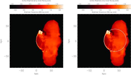
Left: simulated radio emission from model .25E at 50 Myr (log scale). The colour bar shows intensity in mJy arcsec−2 and brightness temperature at 1440 MHz. The image is 170 kpc on a side. In addition to the two bright radio jets, there is diffuse synchrotron emission filling the cocoon created by the jets. The surface brightness of this emission is ≈10–100 times fainter than the jets. Right: same as left-hand panel, but overlaid with the best-fitting radius of curvature (white circle). The radius is 37 kpc.
The length of the tail is vgal × tAGN, where tAGN is the amount of time the AGN has been active. If there is an estimate for the AGN host galaxy velocity, finding the length of the tail would allow the amount of time the AGN has been active to be determined. Note that in Fig. 1 the length of the tail (left to right) is less than the width of the tail (top to bottom), because the jets initially expand outwards faster than vgal. If the AGN remains active, the tail will continue to lengthen and eventually become longer than it is wide.
Radius of curvature
The right-hand panel of Fig. 1 shows the same image with a circle overlaid with R = 37 kpc, the best-fitting radius of curvature for this image. The circle traces both the upper and lower jet and passes through the bright radio lobes where each jet breaks up. Note that the upper lobe is significantly brighter than the lower lobe at this time. The brightness of the lobes and the curvature of the two jets varies with time due to instabilities in the jet propagation and the small random changes in jet direction that we introduce.
The radius of curvature is determined by an automated fitting procedure. We start with a synthetic radio image and consider only the region 28 kpc above and below of the AGN, the approximate extent of the jets. Because the upper and lower jets and lobes can differ significantly in brightness, we find the maximum brightness of any point in each half of the image and exclude points with less than 10 per cent of this brightness. For each slice along the jet, we then determine the horizontal location of the jet by taking an intensity weighted average of the radio emission in that slice. We then fit a circle to the jet locations weighted by the total radio intensity of the points in each slice.
To characterize how much fluctuations in the jet affect the radius of curvature, we use the above procedure to measure the radius of curvature at a series of times (after the jet curvature is well established) and compare the results. Fig. 2 plots measured values of R for simulation.25E from 40 Myr to 220 Myr. The error bars represent the 1-σ error on the value of R at each time, typically about 10 per cent. The values of R are very consistent, with a scatter of about 25 per cent. The best-fitting value of R for simulation.25E is 35.5 ± 7.9 kpc, where the error takes into account both the error in individual fits and variations between different snapshots. The same procedure is applied to all of our simulations, with the results listed as R in Table 1.
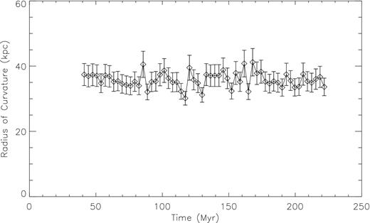
Best-fitting radius of curvature at different times for model .25E. The radius varies about 15 per cent between measurements. The overall mean radius is 35.5 kpc with an error of 7.9 kpc.
Jet thickness
A similar process is used to find the average jet thickness, listed as h in Table 1. The thickness typically has a very small variation, ≃5 per cent, and the accuracy is limited by the resolution of our simulations. Because we are interested in the ‘real’ value of the jet thickness, we determine it using the raw simulation data rather than the synthetic radio data. We take a region of ±24 kpc from the AGN and define points as being in the jet if at least 80 per cent of the material at that point was injected by the nozzle and it is moving with at least 80 per cent of the initial jet velocity. This excludes all material in the lobes and the cocoon around the jet. We then determine the jet thickness perpendicular to both the jet direction and the motion of the AGN, henceforth the ‘z’ direction, as this is the front along which the ram pressure acts. For each slice through the jet, we take the average thickness for points in the jet in the ‘z’ direction. We then take the average of this thickness in all slices to get a value for h at that time, with the standard deviation of the average being the uncertainty at that time. To get the values of h in Table 1, we then find the best-fitting value of the thickness for all times considered, and the error takes into account both the error at individual times and the variation with time.
The overall result is that the radius measured at a particular time is accurate to within an error of 25 per cent of the ‘true’ value for that particular combination of parameters. The thickness is more consistent, with typically only a 5 per cent variation. The variation in R sets a lower limit on the accuracy of the IGM density estimated from the observations of bent-double radio sources.
DISCUSSION
Analytic fit for radius of curvature
We run one model, .015E_theta20, with a small nozzle size and a 20° initial opening angle. The measured values of R and h in Table 1 are 8.6 ± 0.8 kpc and 0.44 ± 0.2 kpc, respectively, very close to the predicted values of 8.5 and 0.49 kpc given by equations (7) and (6). The results are also very similar to model .015E, which has the same setup but with a cylindrical jet input and a 0.5 kpc nozzle size.
Using the measured values of R and h in Table 1 for all of our parallel jet models, we find that the value of h stays very close to the nozzle size and the ratio of h/R is about 1/18, close to the our analytic estimate of 1/17.
Fig. 3 plots the radius of curvature versus jet luminosity for models .015E, .062E, .25E and 1E. These models differ only in jet luminosity, with all other parameters the same. The error bars represent the overall error in measuring R, as discussed in Section 3.1. The solid line is a plot of equation (9) for radius versus luminosity and passes well within the error bars of all the four data points.
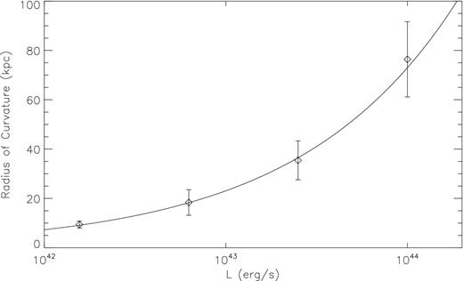
Radius of curvature versus jet luminosity (diamonds) for models .015E,.062E, .25E and 1E. These models differ only in jet luminosity, with all other parameters the same. The error bars represent the overall error in measuring R. Solid line is a plot of equation (9) for radius versus luminosity.
The jet kinetic luminosity calculated using this formula for the sources and measured values of R, h and the synchrotron pressure Pmin in Freeland & Wilcots (2011) are listed in Table 2. The values in Table 2 are upper limits on the luminosity made with the assumptions that the observed value of h is the true jet thickness and that the jet velocity is vjet = c. If the jet is narrower or slower, the luminosities will be smaller. Note that the formula for Ljet is independent of the AGN velocity, so values can be found even for sources with unconstrained velocities. The sources are all of the order of 1045 erg s−1 and the variation between sources is smaller than the variation in the total radio power at 1440 MHz (L1440). Pmin is proportional to L4/7rad, which is the total radio emission at the point where Pmin is measured. Lrad therefore depends on the 1440 MHz emission at that point and the model of the synchrotron spectrum used, but is not directly dependent on the total 1440 MHz emission of the entire source. Pmin scales with jet thickness as h−8/7, so Ljet ∝ h6/7.
Jet kinetic luminosity.
| Source ID | va, bgal | Pamin | naIGM | ha | Rabend | La1440 | Lcjet |
|---|---|---|---|---|---|---|---|
| (km s−1) | 10−11 erg cm−3 | (cm−3) | (kpc) | (kpc) | (W Hz−1) | (erg s−1) | |
| S1 | 430+ 170-35 | 0.9 ± 0.2 | 3 ± 2 × 10⁻³ | 23 ± 1 | 42 ± 6 | 1.6 × 1025 | 1.1 ± 0.2 × 1045 |
| S2 | 570 ± 60d | 0.6 ± 0.2 | 5 ± 4 × 10⁻⁴ | 30 ± 4.5 | 104 ± 9 | 1.88 × 1025 | 1.2 ± 0.5 × 1045 |
| S3 | 745+ 109-80 | 1.4 ± 0.6 | 2 ± 1 × 10⁻⁴ | 10 ± 0.6 | 141 ± 19 | 3 × 10²³ | 3.1 ± 1.4 × 1044 |
| S4 | 950+ 210-140 | 1.7 ± 0.3 | 5 ± 2 × 10⁻⁴ | 22 ± 0.7 | 89 ± 7 | 9.5 × 1024 | 1.5 ± 0.3 × 1045 |
| S5 | Unconstrained | 0.4 ± 0.1 | (70 ± 21)/v2 | 38 ± 3.8 | 220 ± 11 | 6.4 × 1024 | 1.3 ± 0.4 × 1045 |
| S6 | Unconstrained | 0.6 ± 0.1 | (156 ± 48)/v2 | 19 ± 3.1 | 69 ± 4 | 9 × 10²³ | 4.8 ± 1.4 × 1044 |
| S7 | 850+ 170-120 | 1.4 ± 0.3 | 2 ± 1 × 10⁻³ | 22 ± 3.6 | 18 ± 4 | 2 × 1024 | 1.5 ± 0.5 × 1045 |
afrom Freeland & Wilcots (2011).
bvgal here is |$\sqrt{3}$| times the group velocity dispersion, which is listed as vgal in table 1 of Freeland & Wilcots (2011).
cUpper limit, assuming vjet = c.
dFor S2, velocity is based on the difference in redshift between the source galaxy and the group, not the velocity dispersion.
Note that we assume the ram pressure of the jet, Pjet, is accurately reflected by the minimum synchrotron pressure, Pmin, which is true only if the jet energy is dominated by relativistic electrons and magnetic fields. If the true jet ram pressure is higher, the estimates of both nIGM and Ljet in Table 2 will both be proportionally higher. Adding invisible components to the momentum flux of the jet only acts to increase the required IGM density. On a similar note, in our simulations very little external material becomes entrained in the jets. However, even if a significant amount of mass is entrained it will not change the momentum flux of the jet. Therefore, the radius of curvature and inferred IGM density should not be affected. Also note that the equations in this section were derived assuming that the AGN host galaxy is moving supersonically relative to the IGM and that the jet velocity is supersonic relative to its internal sound speed. These relations are not expected to hold if galaxies or jets are subsonic.
Effects of observational resolution
Although the jets are well resolved in our simulations, they are typically unresolved in radio observations. From equations (2) and, the density derived from observations will scale with jet thickness and radius of curvature as nIGM ∝ (h/R)−1/7R−8/7. The values of h/R in our simulations (Table 1) range from about 1/13 to 1/21 with a typical value of about 1/18. The observed ratio (Table 2) ranges from h/R = 1/14 for S3 to h/R = 1/0.83 for S7. Although the density scales weakly with jet thickness, if we assume a real value of h/R = 1/17, corresponding to an initial jet opening angle of θ = 20°, the densities for observed sources would be between 3 per cent (S3) and 54 per cent (S7) higher. If a θ = 5° initial opening angle is assumed, the correction would be between 52 per cent (S3) and 128 per cent (S7) For an under-resolved jet, the observed thickness will always be too high, and therefore the density derived will always be lower than the actual value. This is generally a fairly small correction, about 25 per cent for a typical source, but can be up to 50 per cent or more for sources with hobs ∼ R.
Inadequate resolution can also affect the measurement of the radius of curvature. To characterize this, we apply a Gaussian smoothing filter to our radio images of simulation .25E to simulate radio beam full width at half-maximum (FWHM) sizes from 1 kpc to 32 kpc, and then used our fitting routine to find the radius of curvature. The results are plotted in Fig. 4. For this simulation, the actual radius of curvature is R = 36 kpc and the jet thickness is h = 2 kpc. For a marginally resolved jet (beam size ≤2 kpc) the measured value of R does not change. For larger beam sizes, R is overestimated by about 10 per cent to 25 per cent. As the beam size becomes comparable to the radius of curvature, the fit for R becomes very poor (error comparable to R). Even in this case, however, the measured value of R is systematically larger than the real value. An overestimate of R will lead to an underestimate of the density derived from equation (2), typically about 20 per cent for sources with unresolved jets.
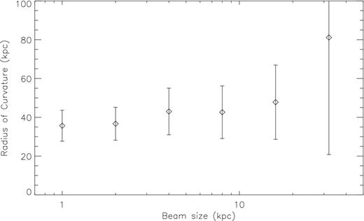
Measured radius of curvature versus beam size for model .25E. The error bars represent the overall error in measuring R. As the beam size increases, the measured R initial remains fairly constant, but then begins to increase, along with the error, as the beam size approaches R. Once the beam size is approximately equal to R, the radius cannot be reliably measured.
Combining the effects of overestimating the jet thickness and overestimating the radius of curvature, we find that for a typical source in Freeland & Wilcots (2011) (resolved source, unresolved jet, h/r ≈ 1/4) the density calculated is low by about 50 per cent, assuming a true value of h/R of 1/17. This ranges from no correction for source S3 (marginally resolved jet) to about 85 per cent low for source S7 (beam size ∼R).
For estimates of the jet luminosity, the error due to resolution can be significantly larger. From equation (12), we find that Ljet ∝ h2Pjet ∝ h6/7. There is no dependence on R, but luminosity is very sensitive to h. For example, assuming a real value of h/R of 1/17, the derived luminosity in Table 2 would be reduced by a factor ranging from 1.2 (S3) to 13 (S7).
Effect of viewing angles
So far, we have produced synthetic images of our simulations assuming that both the direction of jet propagation and the direction of motion of the AGN relative to the IGM are perpendicular to the observer's line of sight. In reality, for observed bent-double radio sources there will be unknown angles between the jet direction and the observer and the direction of motion and the observer, both of which will affect the measurement of the radius of curvature. The angle between the jet and the direction of motion will change where the point of maximum curvature is along the jet, but will not change the radius of curvature at that point (e.g. Begelman et al. 1979).
To quantify how much error viewing angle introduces, we take the data from simulation .25E, rotate it by various angles, then use it to create synthetic radio images. We then measure the radius of curvature in each of these images by the procedure in Section 3.1. Fig. 5 plots the measured radius of curvature for an angle between the jet direction and the observer between 0° and 90°. In all cases, the direction of motion of the AGN is perpendicular to the observer's line of sight. The solid line in Fig. 5 is R = R(θ = 0) × cos (θ), which is the expected apparent radius of curvature of a simple rotated circle. The measured value of R follows this line fairly well out to about 60°, where the apparent radius is half the real radius. Beyond this, the measured radius does not get any smaller. This is because the radio lobes at the ends of the jets begin to overlap from the observer's point of view, and their size dominates the fitting routine. This is one possible explanation for the appearance of source S7 in Freeland & Wilcots (2011), which appears to have a small radius of curvature but with very thick jets. At 90°, the fitting routine fails. However, it is unlikely that a source with the jet aimed almost directly at the observer would be classified as a bent-double radio source.
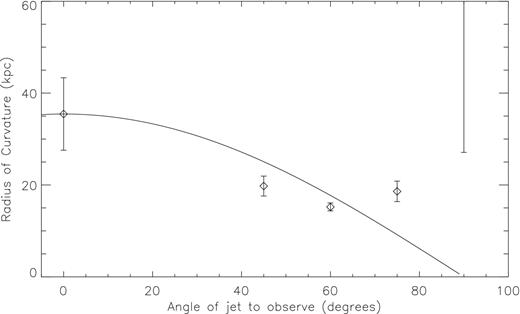
Measured radius of curvature versus angle of jet direction relative to the observer (0° is perpendicular) for simulation.25E. Solid line is R = R(θ = 0) × cos (θ), the expected geometric correction. The measured R follows this line fairly well out to about 60°, beyond which the radius of curvature is poorly fit.
Fig. 6 plots the measured radius of curvature for an angle between the direction motion of the AGN and the observer between 0° and 90°. In all cases, the jet direction is perpendicular to the observer. The solid line is Fig. 6 is R = R(ϕ = 0)/cos (ϕ), which is the expected apparent radius of curvature of a simple circle rotated in the same manner. The measured value of R follows this line out to about 60°, where the apparent radius is double the real radius. Beyond this, the source is so inclined that the jet appears to be approximately straight and the fitting routine fails.
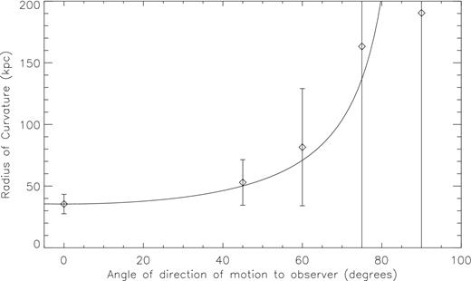
Measured radius of curvature versus angle of direction of motion relative to the observer (0° is perpendicular) for simulation.25E. Solid line is R = R(ϕ = 0)/cos (ϕ), the expected geometric correction. The measured R follows this line fairly well out to about 60°, beyond which the radius of curvature is poorly fit.
In practice, sources will be rotated around both axes, and orientation effects tend to cancel each other out somewhat. Assuming sources rotated beyond 60° in either direction will not be classified as bent-double radio sources, the unknown viewing angle still introduces a large uncertainty in the measurement of R, and therefore in the values of nIGM and Ljet. On average, the error in the measurement of R due to viewing angle should be between 50 per cent low to 30 per cent high (1σ), but for an individual source could be up to a factor of 2 (100 per cent underestimated to 50 per cent overestimated).
X-ray detectability
In general, the gas in galaxy groups is too cool and too low density to be seen in X-ray observations. However, as an AGN moves through the IGM, a cocoon of shocked material develops around the jets. The shock heats and compresses the IGM, boosting the X-ray emission. The parameters that affect the X-ray brightness are the velocity of the AGN, vgal, which determines the temperature of the shocked gas, and the density of the IGM, nIGM, which will determine the emissivity at a given temperature.
To determine if bent-double radio sources in groups would be detectable in X-rays, we used the XIM tool (Heinz & Brüggen 2009) to model 100 ks Chandra observations of four of our simulations, models .015E_.25vel, .062E_.5vel, .25E and 1E_4n, placed at a redshift of z = 0.1. Fig. 7 shows synthetic Chandra images. In all figures, we assume a background IGM temperature of 5 × 10⁵ K and an IGM metallicity of Z = 0.3 solar. All four simulations have about the same radius of curvature of R ≈ 36 kpc. The first three simulations have the same IGM density with AGN velocities of vgal = 250 km s−1 (upper left), 500 km s−1 (upper right) and 1000 km s−1 (lower left). The last two simulations have the same AGN velocity (vgal = 1000 km s−1) but different densities of nIGM = 10−3 cm−3 (lower left) and 4 × 10⁻³ cm−3 (lower right). For these images, we assume there is no point-source emission from the AGN. Even if there is point-source emission, however, the high spatial resolution provided by Chandra would be able to remove this contribution.
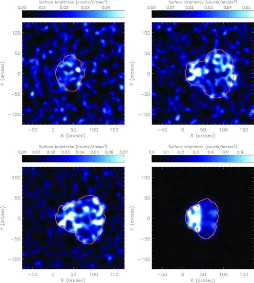
Simulated Chandra X-ray observations for a 100 ks of models .015E_.25vel (upper left), .062E_.5vel (upper right), .25E (bottom left) and 1E_4n (lower right) at a redshift of z = 0.1. All images are the total counts from 0.3 to 3 keV and are smoothed over 10 arcsec. The radius of curvature of the jet in each model is about 36 kpc (20 arcsec). The colour bars show the scale of each image in counts arcsec−2, scaled to 70 per cent of the maximum brightness in each image. The orange contours mark the outer extent of radio emission.
Except in the lowest velocity case, there is significant X-ray emission from the region of the AGN jet and extended tail. We would expect emission to be strongest at the leading edge of the jet, where we are seeing the strongest part of the shock edge-on. However, because the edge-on shock is very thin and significant smoothing is needed to bring out the X-ray emission (10 arcsec in these images), the leading edge does not stand out. Instead, X-ray emission is spread across the region affected by the AGN and dominated by face-on shocks.
In Fig. 8, we plot the mean surface brightness between −50 and +50 arcsec of the AGN along the y-axis (parallel to the jet) in Fig. 7. In the worst-case presented here (model .015E_.25vel, upper left-hand panel), the surface brightness is about 0.02 counts arcsec−2 for a 100 ks exposure, about twice the background level. As the AGN velocity increases, the surface brightness increases as roughly v∼ 0.75gal, reaching about 0.045 counts arcsec−2 for model .25E. For model 1E_4n (lower-right panel), which has the same velocity as model .25E, the brightness increases to 0.3 counts arcsec−2, a scaling of about n∼ 1.5IGM. In all cases, the shocks surrounding the AGN jet and tails are well resolved, so numerical mixing should have a minimal impact on the derived X-ray brightness.
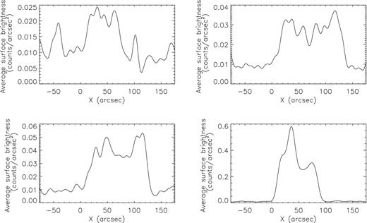
Plots of the mean surface brightness between y = −50 and y = +50 arcsec in each image in Fig. 7 versus x position. Even in the worst case (model .015E_.25vel, upper left), the mean surface brightness is about .02 counts arcsec−2, about twice the background level. This increases roughly as v0.75gal to about .045 counts arcsec−2 for model .25E. For model 1E_4n, which has the same velocity as model .25E, the brightness increases to 0.3 counts arcsec−2, scaling as about n1.5IGM.
If these models were placed at a higher redshift, the angular size of the X-ray source would decrease, but the surface brightness would remain the same. For a large radius of curvature, the thickness of the shocked material, and therefore the surface brightness, will increase proportional to R.
X-ray observations of bent-double radio sources in groups would place important constraints on the IGM properties. The X-ray surface brightness, along with an estimate of vgal from velocity dispersion in the group, would allow nIGM to be calculated independent of the radio observations. Density calculated this way would also be less sensitive to the AGN velocity, scaling as about nIGM∝v∼ −0.5gal rather than nIGM∝v− 2gal as in equation (2). The different scaling also means that in cases where vgal is unconstrained, X-ray and radio data can be combined to find both the IGM density and AGN velocity. This can also be used to refine the vales of vgal and nIGM and constrain the viewing angle in cases where there is an estimate for the AGN velocity. Because the X-ray emission follows the tail of extended radio emission, measuring the length of the X-ray emitting region would provide an age estimate for the source.
For particularly bright sources, there may be enough photons to determine the temperature of the shock. The temperature will scale roughly as T∝v2gal, so if the temperature can be found it would allow vgal and nIGM to be estimated from the X-ray data alone. With additional constraints from radio and velocity dispersion observations, it would then be possible to find the compression ratio of the shock, and from that the temperature of the unshocked IGM.
CONCLUSIONS
Our simulations are able to closely match the appearance of observed bent-double radio sources with narrow, curved jets ending in bright radio lobes. We also predict that there should be an extended tail of radio emission that may be observable at low resolution and/or low frequencies. The length of this tail would allow the age of the AGN to be determined.
From our simulations, we derive a formula for the radius of curvature (equation 9) in terms of IGM density, AGN velocity, jet luminosity and jet velocity. From this, we are able to calculate the kinetic jet luminosity (equation 12) for observed bent-double radio sources, and find that Ljet is typically around 1045 erg s−1, assuming that vjet ≃ c and that the jets are really as thick as their observed values (see Table 2). The luminosities should be considered upper limits, as they will be lower if either the jets are slower or the jets are intrinsically thinner. This formula is independent of vgal and therefore can be used to find Ljet even when the velocity of the AGN is unknown.
A lack of resolution in radio observations leads to a systematic underestimate of the IGM density for two reasons: the jet is unresolved and the radius of curvature is overestimated. In our simulations, we use initial conditions that produce ratio for jet thickness to radius of curvature of h/R ≃ 1/17, equivalent to a 20° initial opening angle of the jet. For observed sources (limited by resolution), this ratio ranged from 1/14 to 1/0.83 in Freeland & Wilcots (2011). Density scales as (h/R)−1/7, so this leads to an underestimate of the IGM density of up to 50 per cent. Inadequate resolution also leads to an overestimate of the radius of curvature (and corresponding underestimate of density), probably by about 20 per cent. Overall, IGM density estimates for typical sources in Freeland & Wilcots (2011) are low by about 50 per cent due to resolution effects. This ranges from no correction for source S3 (assuming a marginally resolved jet) to about 85 per cent low for source S7 (beam size ∼R).
The largest source of error, however, comes from the unknown angles between the observer, the jet direction and direction of motion of the AGN. This can lead to either an over or underestimate of the true radius of curvature. This leads to an uncertainty of up to a factor of 2 in the estimate of the IGM density, with a typical (1σ) error or about 50 per cent. This is comparable to the error from all observational uncertainties (dominated by the uncertainty in the AGN velocity). Even this uncertainty, however, does not change the conclusion that bending can be used to diagnose ρIGM in a statistical sense.
Finally, we have modelled the X-ray emission of bent-double radio sources and predict that they should be detectable in Chandra X-ray observations. Although the IGM in groups is generally too cool and diffuse to be seen in X-ray observations, the shocks around the jet and tail in our simulations compress and heat the IGM, potentially making the entire region affected by the AGN jets detectable in X-rays. The X-ray surface brightness scales as approximately S∝n1.5IGMvgal0.75. Sources in fairly dense environments and with fairly large angular size should be detectable in moderate (∼100 ks) observations. Count rates from existing short X-ray observations of sources S1 and S2 in Freeland et al. (2008) are consistent with our predictions. Furthermore, X-ray observations would provide complimentary constraints on the IGM density and AGN velocity to radio observations.
For particularly bright sources, it may be possible to obtain a measure of the temperature of the shock from X-ray observations. This would provide an independent measure of the AGN velocity relative to the IGM.
Futuremore, X-ray and radio observations will be able to place better constraints on the IGM density, AGN velocity and AGN age. With very complete observations it should also be possible to constrain the temperature of the IGM and the orientation of the jets and direction of AGN motion.
BJM is supported by an NSF Astronomy and Astrophysics Postdoctoral Fellowship under award AST1102796. BJM and SH acknowledge NSF grant AST0707682. SH acknowledges NSF grant AST1109347. MB acknowledges support by the research group FOR 1254 funded by the Deutsche Forschungsgemeinschaft (DFG). MR acknowledges NSF grant 1008454. The software used in this work was in part developed by the DOE NNSA-ASC OASCR Flash Center at the University of Chicago. Resources supporting this work were provided by the NASA High-End Computing (HEC) Program through the NASA Advanced Supercomputing (NAS) Division at Ames Research Center.
NSF Astronomy and Astrophysics Postdoctoral Fellow.
