


Abstract
We present CHAOS-4, a new version in the CHAOS model series, which aims to describe the Earth's magnetic field with high spatial and temporal resolution. Terms up to spherical degree of at least n = 85 for the lithospheric field, and up to n = 16 for the time-varying core field are robustly determined.
More than 14 yr of data from the satellites Ørsted, CHAMP and SAC-C, augmented with magnetic observatory monthly mean values have been used for this model. Maximum spherical harmonic degree of the static (lithospheric) field is n = 100. The core field is expressed by spherical harmonic expansion coefficients up to n = 20; its time-evolution is described by order six splines, with 6-month knot spacing, spanning the time interval 1997.0–2013.5. The third time derivative of the squared radial magnetic field component is regularized at the core–mantle boundary. No spatial regularization is applied to the core field, but the high-degree lithospheric field is regularized for n > 85.
CHAOS-4 model is derived by merging two submodels: its low-degree part has been derived using similar model parametrization and data sets as used for previous CHAOS models (but of course including more recent data), while its high-degree lithospheric field part is solely determined from low-altitude CHAMP satellite observations taken during the last 2 yr (2008 September–2010 September) of the mission. We obtain a good agreement with other recent lithospheric field models like MF7 for degrees up to n = 85, confirming that lithospheric field structures down to a horizontal wavelength of 500 km are currently robustly determined.
1 INTRODUCTION
More than 14 yr of continuous magnetic field measurements collected by the Ørsted and CHAMP satellites present outstanding opportunities to investigate the Earth's magnetic field, both regarding rapid changes of the core field (secular variation) and the determination of the magnetic field due to lithospheric magnetization.
Of special interest for deriving the small-scale structure of the lithospheric field are the measurements obtained during the final months of the CHAMP satellite mission, when the satellite altitude was below 300 km. The benefit of low-altitude CHAMP observations for determining the lithospheric field is obvious from Fig. 1, which shows the spatial power spectrum of the geomagnetic field at various altitudes. The black curve is the lithospheric power at Earth's surface (according to the CHAOS-4 model presented in this article), while the coloured curves present spectra at various altitudes of CHAMP (blue curves) and of the Ørsted satellite (red curve).
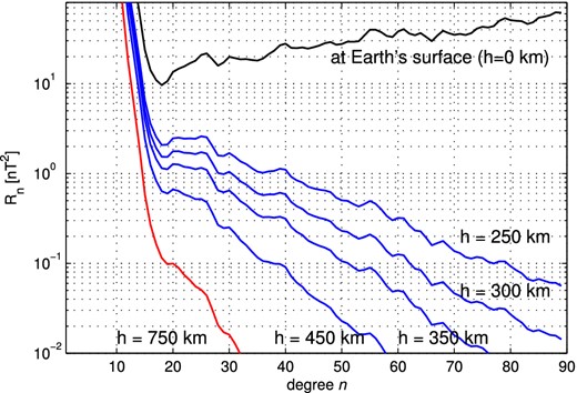
Spatial power spectrum of the geomagnetic field at Earth's surface (black curve) and at various altitudes of CHAMP (blue). Also shown is the spectrum at a mean altitude of the Ørsted satellite of 750 km (red).
Let us assume that measuring conditions (including instrument errors, external field disturbances and spatio-temporal sampling) are such that magnetic field structures of squared amplitudes larger than 0.1 nT2 can be resolved. Under this assumption only features up to spherical harmonic degree n = 20 can be determined from data obtained by a satellite at an altitude of 750 km (for example, Ørsted). In contrast, data from CHAMP at the beginning of its mission, when altitude was about 450 km, would allow for a determination of the lithospheric field up to n = 40. Data taken at 300 km altitude (which was the mean altitude of CHAMP at the beginning of 2010) would allow the determination of models up to n = 60. Finally, taking advantage of the very-low altitude data from the last weeks of CHAMP mission lifetime, as is done in this paper, would allow the lithospheric field up to n = 80 to be resolved. Note that a threshold value of 0.1 nT2 has been chosen here for illustration purposes only; we do not claim that this is the actual accuracy of the magnetic satellite data.
As described in the review article by Thébault et al. (2010), two complementary philosophies are currently adopted when deriving spherical harmonic models of the Earth's lithospheric field. In the sequential approach, a-priori models of all known magnetic field contributions, except for the lithospheric field, are subtracted from the data, followed by a careful data selection and application of empirical corrections. The different versions in the MF model series derived by Stefan Maus and co-workers (cf. Maus et al.2002, 2006, 2007, 2008) are examples of models determined using this approach. They are derived from CHAMP observations which have been along-track filtered after removal of a priori models of the core field and of the ocean tidal magnetic signal. MF6, the most recent published model version (Maus et al.2008), also includes line levelling between adjacent satellite tracks, which minimizes the variance between close encounters. This model formally describes the lithospheric field up to spherical harmonic degree n = 120 (corresponding to 333 km horizontal wavelength), but coefficients above n > 80 are damped (regularized) and thus probably not robustly resolved. A new (unpublished) version, MF7 (Maus 2010), describes the field formally up to n = 133.
Contrary to this serial approach, the comprehensive approach aims to solve simultaneously for all major internal and external field contributions. Examples of models derived using this approach are the CM models (e.g. Sabaka et al.2004), and, using more recent satellite data, the GRIMM models (Lesur et al.2008; Lesur et al.2010, 2013), the BGS models (Thomson & Lesur 2007; Thomson et al.2010), and the CHAOS models (Olsen et al.2006, 2009, 2010).
Until recently, the altitude of the CHAMP satellite was not sufficiently low to determine small-scale structures of the lithospheric field without along-track filtering of the data (to remove unmodelled external field contributions), and hence only terms up to spherical harmonic degree n = 50 or so could be determined robustly using the comprehensive approach. Inclusion of the most recent low-altitude CHAMP data, as done here, allows determination of the lithospheric field up to at least spherical harmonic degree n = 85.
The very recent low-altitude CHAMP observations are crucial for a robust determination of small-scale lithospheric field structures. But how has CHAMP altitude evolved with time? The left-hand part of Fig. 2 shows in blue the altitude of CHAMP (with respect to a mean Earth radius of a = 6371.2 km), together with the temporal evolution of the F10.7 solar flux (red curve). Various orbit manoeuvres are the reasons for sudden increases of the satellite altitude. Note how rising solar activity at the end of 2001 leads to a faster altitude decay, due to increased air density and thereby larger air-drag.
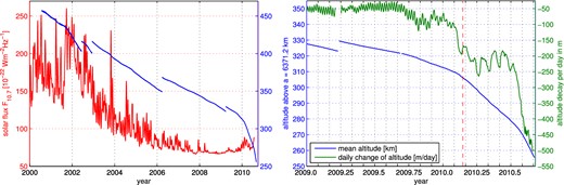
Left-hand panel: solar flux index, F10.7 (red) and CHAMP mean altitude (blue) in dependence on time. Right-hand panel: CHAMP mean altitude (blue) and mean daily altitude decay (green) since 2009.
CHAMP altitude was about 350 km during the solar minimum years 2007–2009 and reached 300 km at the beginning of 2010. The satellite altitude for the last 2 yr of mission lifetime is shown in the right-hand part of Fig. 2, together with the mean daily change of altitude (green curve). The latter was about 50 m/d in 2009, but increased to a value of about 200 m/d during the first part of 2010, partly due to the fact that the satellite was turned by 180°. Before 2010 February 22 (indicated by the dashed red vertical line) CHAMP flew with its boom in the flight direction, which is a favourable condition regarding air drag, but is less optimal for attitude control. After that date CHAMP flew with the boom backward, requiring less cold gas for attitude control. After 2010 July the daily altitude decay increased rapidly to values of 500 m/d and more.
The CHAOS-4 field model presented here is the most recent version in the CHAOS model series. Previous versions are CHAOS (Olsen et al.2006), xCHAOS (Olsen & Mandea 2008), CHAOS-2 (Olsen et al.2009) and CHAOS-3 (Olsen et al.2010). In previous model versions we have concentrated on an optimal description of the core field and its temporal evolution; the static (lithospheric) field was only modelled up to relatively low spherical harmonic degrees (n = 60 at most). For CHAOS-4 we extend the spherical harmonic degrees and solve for the lithospheric field up to n = 100.
However, CHAMP data are not available after 2010 September since the satellite re-entered the atmosphere on 2010 September 19. In order to describe properly the time changes of the core field until mid-2013 we take advantage of the most recent scalar magnetic field observations from the Ørsted satellite and data from magnetic observatories.
CHAOS-4 is derived by merging two models, both of which are determined using the comprehensive approach but from different data sets (and using different model parameterization): spherical harmonic coefficients of the CHAOS-4 model up to degree n = 24 (which includes the time-changes of the core field) are taken from model version CHAOS-4l, while coefficients describing the lithospheric field for n = 25–100 are taken from model version CHAOS-4h. The former is derived in the tradition of the earlier versions of the CHAOS series by using data between 1997.0 and 2013.5 from the three satellites Ørsted, CHAMP and SAC-C together with observatory monthly mean values, while CHAOS-4h is derived solely from the final 2 yr of low altitude CHAMP satellite data.
2 DATA SELECTION
2.1 Satellite data
We use Ørsted scalar data between 1999 March and 2013 June, Ørsted vector data between 1999 March and 2004 December, CHAMP vector and scalar data between 2000 August and 2010 September, and SAC-C scalar data between 2001 January and 2004 December. Similar data selection criteria to those chosen for determining previous versions in the CHAOS model series have been used; the main modification concerns the use of quasi-dipole (QD) latitude (Richmond 1995) instead of dipole latitude to distinguish polar from non-polar regions, and use of a revised version of the dayside merging electric field at the magnetopause when selecting data at polar latitudes and the inclusion of pre-midnight CHAMP data: for previous CHAOS versions we only used post-midnight non-polar CHAMP data to avoid contamination of the lithospheric field determination by plasma irregularities. However, these irregularities are almost absent during the solar minimum conditions of the recent years which we used to determine the lithospheric field, allowing us to include also pre-midnight data.
All satellite data are weighted proportional to sin θ (where θ is geographic colatitude) to simulate an equal-area distribution. Anisotropic errors due to attitude uncertainty (Holme & Bloxham 1996; Holme 2000) are considered for all Ørsted vector data and for CHAMP vector data when attitude data from only one star imager were available.
In order to obtain a core field model that is up-to-date we included most recent Ørsted scalar field observations, up to 2013 June. The top panel of Fig. 3 shows the total number of non-polar magnetic satellite observations for each month. Periods with fewer data (for instance around 2003) are due to increased geomagnetic activity, while problems with the attitude stability are the reason for the Ørsted data gap around 2007 and after 2011. Beginning in 2012 November special efforts have been undertaken to improve the retrieval of Ørsted data in order to better bridge the gap between the atmospheric re-entry of CHAMP and the launch of Swarm. This has resulted in significantly more data since end of 2012. All Ørsted data, including the very recent ones, are freely available at ftp.space.dtu.dk/data/magnetic-satellites/Oersted/.
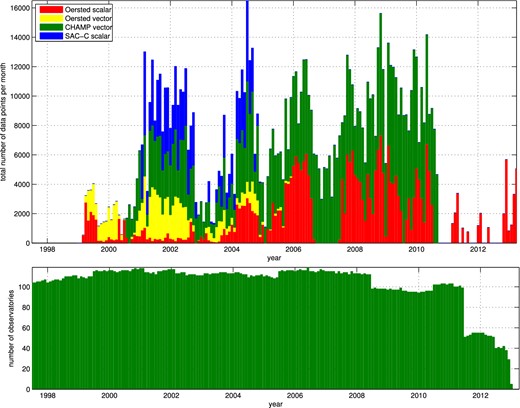
Top panel: total number of non-polar satellite data (stacked histogram) as a function of time. Bottom panel: number of magnetic observatory monthly mean values as a function of time.
2.2 Ground data and the RC index describing the magnetospheric ring-current
The time-space structure of the magnetospheric field is traditionally described by the Dst index (e.g. Sugiura 1964). However, the baseline of Dst is known to change with time (e.g. Olsen et al.2005; Lühr & Maus 2010), which hampers its use in geomagnetic field modelling. We therefore derived a new index, called RC, which describes the strength of the magnetospheric ring-current even during geomagnetic quiet conditions (when the baseline instabilities of Dst lead to less-optimal results). RC is derived by an hour-by-hour spherical harmonic analysis (SHA) of hourly mean values from worldwide distributed observatories at mid and low latitudes. The locations of the 21 observatories used to derive RC in this study are indicated by red dots in Fig. 4.
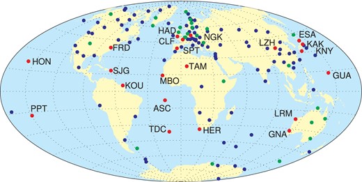
Location of the 146 magnetic observatories used in this study (circles). Emphasized (green or red symbols) are the 43 observatories that provided quasi-definitive (cf. Peltier & Chulliat 2010) data in 2013, out of which 21 observatories (red dots with three letter code given) were used for calculating the RC index.
After removal of the core field as given by a preliminary version of CHAOS-4 from the hourly mean values, an observatory bias (accounting for the high-degree lithospheric field that is not described by that model) was subtracted from each component at each observatory. This observatory bias was determined such that the arithmetic mean value during geomagnetic quiet periods (defined as Kp ≤ 20, |dDst/dt| ≤ 2 nT hr−1) vanishes. Next, all data were converted from the geographic to the dipole (geomagnetic) frame. We then performed an hour-by-hour spherical harmonic analysis on the horizontal components, estimating time series of the three spherical harmonic expansion coefficients |$v_1^m$| of degree n = 1 and order m = 0 and 1. For this spherical harmonic analysis we used only those observatories that were (for the UT hour in consideration) located in the night-side sector (local time between 18 and 06). Due to this selection only between 5 (for UT = 08) and 16 (for UT = 20) out of the 21 observatories have been used, with the number of observatories changing from hour to hour.
The RC index is defined as |$RC=-v_1^0$|; the minus sign is introduced in order to make RC compatible to the definition of Dst as the southward component of the magnetic field at the dipole equator.
Since RC is derived from the horizontal components only, it consists of the sum of magnetospheric and induced part, similar to Dst [this is the reason why we denote the spherical harmonic expansion coefficients as |$v_1^m$|; it is the sum of the external (magnetospheric) coefficient |$q_1^m$| and the internal (induced) coefficient |$g_1^ m$|]. In a final step we decompose RC(t) = ϵ(t) + ι(t) into external and induced parts, respectively, using a 1-D model of electrical conductivity of the mantle as described in Olsen et al. (2005).
To stabilize the determination of the CHAOS-4 core field time changes and to extend it back in time before February 1999 (the launch of the Ørsted satellite) we supplement the satellite data with annual differences of revised observatory monthly means of the north, east and vertical downward components (X, Y, Z) for the time interval 1997.5 to 2013.5. These monthly means have been derived from hourly mean values of 146 observatories (shown in Fig. 4) which have been carefully checked for trends, spikes and other errors as described in Macmillan & Olsen (2013). We removed from the observations (i) synthetic model values of the ionospheric (plus induced) field as predicted by the CM4 model (Sabaka et al.2004), which takes as input 3-monthly means of F10.7 solar flux and (ii) model values for the magnetospheric (plus induced) field as predicted by a preliminary version of CHAOS-4, parametrized by the RC index and its decomposition into external and induced parts. After subtracting these field corrections from the observed hourly mean values we calculate the robust mean [using Huber weights with a tuning constant of 1.5, cf. Huber (2011)] of all hourly mean values of a given month, for each of the 146 observatories and each of the three elements X, Y and Z. Finally, we take the annual differences of the resulting revised monthly means (annual difference value at time t is obtained by taking the difference between those at t + 6 months and t − 6 months to eliminate a remaining annual variation in the data). This yields 19 299 values of the first time derivative of the vector components, dX/dt, dY/dt, dZ/dt, for 146 observatories. Their distribution in time is given in the bottom panel of Fig. 3.
3 MODEL PARAMETRIZATION
Parametrization of the CHAOS-4 model follows closely that of the previous versions in the CHAOS model series. The model consists of spherical harmonic expansion coefficients describing the magnetic field vector in an Earth-centred earth-fixed (ECEF) coordinate system and sets of Euler angles needed to rotate the satellite vector readings from the magnetometer frame to the star imager frame. The magnetic field vector in the ECEF frame, B = −∇V, is derived from a magnetic scalar potential V = Vint + Vext consisting of a part, Vint, describing internal (core and lithospheric) sources, and a part, Vext, describing external (mainly magnetospheric) sources and their Earth-induced counterparts. Both parts are expanded in terms of spherical harmonics.
As mentioned above, the final CHAOS-4 model is found by merging two submodels, called CHAOS-4l, resp. CHAOS-4h. They differ in the maximum spherical harmonic degree Nint of the static field, in the temporal parametrization of the low-degree (core field) terms, and in the data sets that have been used to derive these submodels. Details are given below in Sections 3.1 and 3.2.
In the following we describe in more detail the data and model parametrization used for the two submodels CHAOS-4l and CHAOS-4h.
3.1 CHAOS-4l
CHAOS-4l (where the ‘l’ stands for ‘low degree’) is determined using the whole data set (Ørsted, CHAMP and SAC-C satellite data plus observatory monthly means) described above, with a sampling rate of the satellite data of 60 s.
The maximum spherical harmonic degree of the internal field, Nint = 80, is higher than that of CHAOS-2 and CHAOS-3. Internal Gauss coefficients |$\lbrace g_n^m(t),h_n^m(t)\rbrace$| up to n = 20 are time-dependent; this dependence is described by order 6 B-splines (Schumaker 1981; De Boor 2001) with a 6-month knot separation and fivefold knots at the endpoints t = 1997.0 and t = 2013.5. This yields 32 interior knots (at 1997.5, 1998.0, …, 2013.0) and six exterior knots at each endpoint, 1997.0 and 2013.5, resulting in 38 basic B-spline functions Ml(t). Internal Gauss coefficients for degrees n = 21–80 are static. Time-dependent terms (for degrees n = 1–20) and static terms (for n = 21–80) together result in a total of 22 840 internal Gauss coefficients.
The total number of external field parameters is 1230, which is the sum of five SM terms (|$q_2^m, s_2^m$| for m = 0 − 2), 3 RC regression coefficients |$\tilde{q}_1^0, \tilde{q}_1^1, \tilde{s}_1^1$|, two GSM coefficients (|$q_n^{1, {\rm GSM}}, q_n^{2, {\rm GSM}}$|), 900 baseline corrections |$\Delta q_1^0$| and 2 × 160 baseline corrections |$\Delta q_1^1, \Delta s_1^1$|.
Regularization of the third time derivative alone leads to unconstrained field oscillations. To avoid this we also minimize |$|\frac{\partial ^2 {B_r}}{\partial t^2}|$| at the core surface at the model endpoints t = 1997.0 and 2013.5. This is implemented via the regularization matrix |$\underline{\underline{\Lambda }}_2$|. Note that |$\underline{\underline{\Lambda }}_2$| only acts on 12 (the first and last six) of the 38 spline basis functions.
The two parameters λ3 and λ2 control the strength of the regularizations. We considered several values for these parameters and finally selected λ2 = 10 (nT yr−2)−2 and λ3 = 0.33 (nT yr−3)−2. The axial dipole coefficient |$g_1^0$| is treated separately, with λ3 increased to 10 (nT yr−3)−2, since it is the internal field coefficient most affected by unmodelled external field fluctuations.
3.2 CHAOS-4h
CHAOS-4h is the high-degree part of the CHAOS-4 model (as indicated by the suffix ‘h’). The maximum spherical harmonic degree of the internal model part is Nint = 100. CHAOS-4h is derived solely from CHAMP data obtained between 2008 September and 2010 September. The data sampling interval is 30 s. A quadratic time dependence is used to describe the temporal variation of core field coefficients up to degree n = 16; coefficients between n = 17–100 are assumed to be static. This results in a total of 10 776 internal Gauss coefficients. The number of model parameters describing the external field is 1579. Euler angles of the transformation between the magnetometer and the star sensor frame are solved for in bins of 10 d, resulting in 3 × 72 = 216 additional model parameters. In total model CHAOS-4h consists of 12 571 model parameters which are estimated from 118 184 scalar data and 3 × 313 840 vector data.
When estimating high-degree magnetic field models using near-polar orbiting satellites, special attention has to be paid to the polar gaps, which are the regions around the geographic poles of half-angle |90° − i| where i is the inclination of the orbit. Inclination of the CHAMP orbit is i = 87.3°, which results in a polar gap of half-angle 2.7°. Such a gap is especially problematic for the proper determination of zonal coefficients |$g_n^0$| above n = 60. To avoid ringing at the poles we therefore add 1800 synthetic field values of Br, synthesized within the polar gap from model CHAOS-4l up to degree n = 60. This suppresses the zonal coefficients |$g_n^0$| for n > 60.
3.3 Merging the two submodels CHAOS-4l and CHAOS-4h
The final CHAOS-4 model is obtained by combining the spherical harmonic coefficients of the two submodels CHAOS-4l and CHAOS-4h. Spherical harmonic coefficients up to n = 24 (which includes the time-changing core field) and the external field are taken from CHAOS-4l, while the lithospheric field coefficients for degrees n = 25–100 are taken from CHAOS-4h. The transition occurs at degree n = 25 where the degree correlation ρn between the two models reaches a maximum of ρn = 0.999 while their relative difference (degree variance of model difference divided by degree variance of CHAOS-4) is less than 0.2 per cent. For all degrees up to n = 50 the correlation ρn > 0.996 and the relative variance difference is below 1 per cent.
4 RESULTS AND DISCUSSION
The total number of data points, residual means and rms values of the two submodels are listed in Table 1. Means and rms are the weighted values calculated from the model residuals e = dobs − dmod using the Huber weights obtained in the final iteration. The statistics of model version CHAOS-4h, with rms values of about 1.8 nT for the scalar field and of 2.2–2.4 nT for the two remaining vector components, impressively demonstrate the capability of CHAMP. The rms values of model version CHAOS-4l are somewhat larger, which is likely due to the longer time span of that model (14 yr compared to only 2 yr for CHAOS-4h), the probably less optimal data quality at the beginning of the CHAMP mission, and the fact that data from four different sources (Ørsted, CHAMP, SAC-C and magnetic observatories) have been combined. The reason for the larger CHAMP residuals compared to the two other satellites is likely due to its lower altitude, which means it is closer to the disturbing ionosphere as well as to unmodelled signals from the lithosphere.
Number N of data points, mean and rms misfit (in nT for the satellite data, and in nT yr−1 for the observatory data) for CHAOS-4l and CHAOS-4h. Statistics for the vector components are given in the (Br, Bθ, Bϕ) coordinate system and in a coordinate system (B2, B⊥, B3) defined by the bore-sight of the star imager and the ambient field direction (cf. Olsen et al.2000, for details).
| CHAOS-4l | CHAOS-4h | |||||||
|---|---|---|---|---|---|---|---|---|
| Component | N | Mean | Rms | N | Mean | Rms | ||
| Satellite | Ørsted | Fpolar | 122,363 | 0.37 | 3.35 | |||
| Br | 89,833 | –0.14 | 5.13 | |||||
| Bθ | 89,833 | –0.24 | 5.23 | |||||
| Bϕ | 89,833 | –0.05 | 4.60 | |||||
| Fnonpolar + BB | 389,229 | 0.13 | 2.35 | |||||
| B⊥ | 89,833 | –0.04 | 7.40 | |||||
| B3 | 89,833 | 0.12 | 3.40 | |||||
| CHAMP | Fpolar | 190,578 | –0.30 | 4.85 | 118,184 | 0.02 | 4.16 | |
| Br | 542,265 | 0.03 | 2.56 | 313,840 | 0.00 | 1.83 | ||
| Bθ | 542,265 | 0.05 | 3.58 | 313,840 | 0.05 | 2.46 | ||
| Bϕ | 542,265 | 0.14 | 2.95 | 313,840 | 0.00 | 2.11 | ||
| Fnonpolar + BB | 542,265 | –0.11 | 2.10 | 313,840 | 0.00 | 1.68 | ||
| B⊥ | 542,265 | –0.02 | 3.36 | 313,840 | –0.02 | 2.27 | ||
| B3 | 542,265 | 0.06 | 3.47 | 313,840 | 0.07 | 2.51 | ||
| SAC-C | Fpolar | 26,051 | 0.54 | 3.81 | ||||
| Fnonpolar | 89,388 | 0.41 | 2.69 | |||||
| Observatory | dBr/dt | 19,299 | 0.11 | 3.78 | ||||
| dBθ/dt | 19,299 | –0.13 | 3.80 | |||||
| dBϕ/dt | 19,299 | –0.02 | 2.98 | |||||
4.1 The lithospheric field
The left-hand part of Fig. 5 shows the spatial power spectrum of CHAOS-4 (black dots) and of various versions of the MF model series determined by Stefan Maus and co-workers. Up to spherical harmonic degree n = 80 the power of CHAOS-4 is very similar to that of MF7 (Maus 2010), which is the most recent version in the MF model series. The power of previous versions in the MF series is smaller than that of MF7 and CHAOS-4. Noteworthy is how the spectral power of the MF models increases with increasing version number: for degrees n = 16–60 the power of MF5 is 15 per cent below that of CHAOS-4 while for the later versions MF6 and MF7 it is similar to that of CHAOS-4 within 1 per cent. For higher degrees (n = 61–80) the power of MF6 is as much as 30 per cent below that of CHAOS-4. The power of the lithospheric signal in MF7 has increased compared to that in MF6 and is very close to that of CHAOS-4. This change in power illustrates the effect of high-pass filtering that was applied in the determination of the MF models; earlier model versions have been derived using heavier filtering compared to more recent versions, resulting in an underestimation of the lithospheric signal. Thébault et al. (2012) discuss the pros and cons of an along-track filtering on the determination of the lithospheric field.
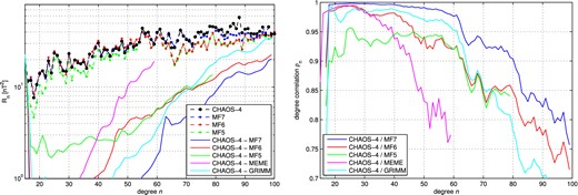
Left-hand panel: power spectra of the static field (dots) and of the field differences (solid lines). Right-hand panel: degree correlation between various model pairs.
Filtering has been relaxed in the most recent versions of the MF series, which clearly results in a stronger lithospheric field. For MF7 filtering is only applied for degrees above n = 77; up to that degree the lithospheric field of CHAOS-4 and MF7 are very similar. But following the argument of the above results, it seems possible that MF7 may underestimate the lithospheric signal for degrees above n = 77, when filtering is again applied. The Swarm constellation mission consisting of three identical satellites, two of which are flying side-by-side at low altitude, will give an excellent opportunity to investigate this further. Experiments based on Swarm-type synthetic data indicate that the lithospheric field up to degree n = 150 can be robustly determined without along-track filtering (Sabaka & Olsen 2006; Olsen et al.2007; Tøffner-Clausen et al.2010; Sabaka et al.2013).
In addition to the spectra of the various lithospheric field signals, the left-hand part of Fig. 5 shows the spectra of the differences between CHAOS-4 and various other field models. The difference is smallest when comparing CHAOS-4 with MF7 which gives an indication of the present uncertainty in lithospheric field modelling. The fact that the lithospheric field power is well above the power of the difference between CHAOS-4 and MF7—two models which have been derived using rather different approaches—confirms that lithospheric field structures up to at least degree n = 80, corresponding to a horizontal wavelength of 500 km, are currently robustly determined.
The right-hand part of Fig. 5 shows the degree correlation ρn [see eq. 4.23 of Langel & Hinze (1998) for a definition] between CHAOS-4 and various other field models. The highest correlation is obtained with MF7, where the degree correlation is above 0.97 for n ≤ 60 and above 0.85 for n ≤ 80.
The left-hand part of Fig. 6 shows the sensitivity matrix S(n, m), which is the relative difference between each coefficient of CHAOS-4 and MF7 in a degree versus order matrix; the right-hand part shows S(n, m) of the difference between CHAOS-4 and MF6. This figure confirms the better agreement between CHAOS-4 and MF7 compared to MF6. There exist, however, certain spherical harmonic orders for which the difference between CHAOS-4 and MF7 is especially large, for instance around m = 60. The reason for these differences is unknown.
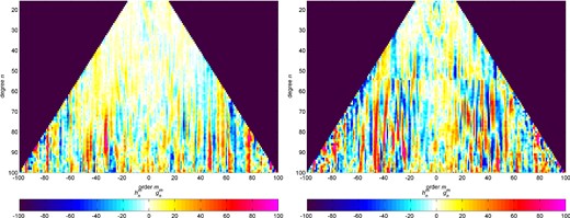
Sensitivity matrix (normalized coefficient differences in per cent) between CHAOS-4 and MF7 (left-hand panel), resp. MF6 (right-hand panel).
A map of the radial magnetic field at Earth's surface, calculated from coefficients between degrees n = 16 and 85, is shown in the upper part of Fig. 7. The bottom part shows the difference in Br between CHAOS-4 and MF7. The largest differences occur in polar regions: Maximum field difference is 55 nT (75 nT) at Northern (Southern) polar latitudes while maximum difference at non-polar latitudes is only 33 nT. This indicates the challenge of proper lithospheric field determination in the vicinity of the ever present magnetic external field perturbations at high latitudes. The reason for the north–south oriented stripes at non-polar latitudes is not clear; it could be caused by contamination from unmodelled magnetospheric contributions in CHAOS-4 or due to the along-track filtering used during the derivation of MF7.
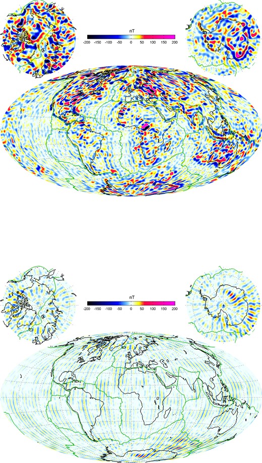
Top panel: map of the radial lithospheric magnetic field at ground, calculated from coefficients of degrees n = 16–85. Bottom panel: radial field differences between CHAOS-4 and MF7.
4.2 The core field, secular variation and secular acceleration
An important question is how well we are able to model the time changes in the core field, especially after 2010 September when only the Ørsted satellite and observatory monthly means are available. Fig. 8 shows the secular variation (SV) and secular acceleration (SA) spectra for various epochs. The colour of the spectrum indicates the model epoch, varying from blue (for t0 = 2000.0) to red (for t0 = 2012.0). We find similar power spectra for the SV captured in CHAOS-4 before and after 2010 September, with no obvious discontinuity. There is considerable time-dependence in the SA spectra below degree 8, also after 2010, while above degree 12 the form of the spectra is essentially controlled by the temporal regularization.
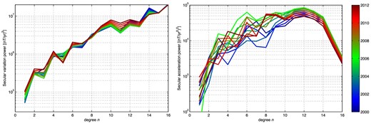
Mauersberger-Lowes spectra of first (left-hand panel) and second (right-hand panel) time derivatives at the core surface. The different curves correspond to different epochs t0 indicated by the colour, from t0 = 2000.0 (blue) in steps of 1 yr until t0 = 2012.0 (red).
Fig. 9 presents annual differences of revised monthly means, in dipole co-ordinates, from the observatories Kakioka – KAK (Japan), MBour - MBO (Senegal) and Canberra – CNB (Australia) together with SV predictions from both the CHAOS-4 model and an earlier version CHAOS-4α, derived in 2010 December. Both models do an excellent job of fitting the observations, particularly when the scatter is low (e.g. KAK dBr/dt, dBϕ/dt; MBO, dBr/dt; CNB dBr/dt). The extrapolation of CHAOS-4α to beyond 2010 September notably fails (e.g. MBO dBθ/dt, CNB dBθ/dt) while CHAOS-4 does better, illustrating its reliability in the post-CHAMP era. CHAOS-4 also does a much better job at fitting rapid changes in the Atlantic region that have occurred since 2009 (e.g. in dBr/dt at MBO, also in dBr/dt at Ascension Island and in Hermanus, South Africa not shown). Localized, rapid, core field changes, particularly at mid-to-low latitudes have previously been studied by Olsen & Mandea (2008) and Chulliat et al. (2010); the latest CHAOS-4 model is evidently suitable for further study of such events, since it succeeds in capturing the amplitude and phase of the latest rapid field changes, especially in the low latitude Atlantic sector.
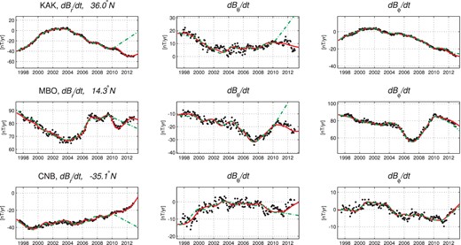
Annual differences of revised magnetic observatory monthly means (black dots) compared to predictions from CHAOS-4 (red line) and from the earlier CHAOS-4α (green dashed line). Top row is Kakioka, Japan, middle row is MBour, Senegal, bottom row is Canberra, Australia.
Fig. 10 presents a map of the radial component of the SV in 2008, truncated at spherical harmonic degree n = 15 and plotted at the core surface. As previously pointed out by Holme et al. (2011), the SV is noticeably low under the Pacific, with the strongest SV generally occurring under the Atlantic hemisphere. Finlay et al. (2012) proposed that enhanced SV under the Atlantic was due to a planetary scale quasi-geostrophic gyre seen in this region in frozen flux core flow inversions (Pais & Jault 2008; Gillet et al.2009). Aubert et al. (2013) have recently presented a new, self-consistent, geodynamo model that demonstrates how the coupled dynamics of the inner core, outer core and mantle system can produce this gyre and the general concentration of SV at mid-to-low latitudes under the Atlantic hemisphere as seen in Fig. 10.
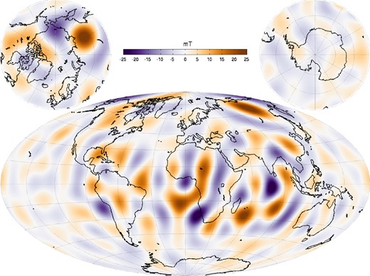
Secular variation of the radial magnetic field component, dBr/dt, up to degree n = 15. Plotted at the core surface for 2008.0.
Looking at the SV at the core surface in the polar regions, Fig. 10 provides further evidence that the SV is very low in the Southern polar regions (see also Holme et al.2011), while in the northern polar region there is a pair of intense, large scale, SV patches. These are related to the present westward motion of a prominent flux patch located under Siberia (Bloxham & Gubbins 1985) and the evolution of a similar patch under Canada/Alaska. Although there are similar high latitude flux patches in the Southern hemisphere, these do not change in such a consistent fashion, hence they generate little SV. This difference in SV between the northern and southern hemisphere polar regions is likely related to different core flows within the northern and southern tangent cylinders in the outer core. The tangent cylinder acts as a dynamic barrier due the Proudman-Taylor theorem, giving rise to different, essentially decoupled, dynamics inside the two polar regions (Olson & Aurnou 1999; Sreenivasan & Jones 2005). Our results suggest there may be westward flow within the northern tangent cylinder but not within the southern tangent cylinder.
Next, we turn to the second time derivative of the core field, also known as the secular acceleration or SA. Chulliat et al. (2010) have pointed out that there was a large peak in the SA at the core surface in 2006. They showed how this pulse event effectively produced jerk signatures in the field at Earth's surface in 2003 and 2007. In Fig. 11, we plot the SA power at the core surface [following Chulliat et al. (2010)], summed over spherical harmonics up to degree n = 8, for which the time-dependence in the SA is well determined. In CHAOS-4 we find not only a dominant peak in 2006, as was the case in earlier members of the CHAOS model series, but also a secondary maximum in 2009. This second peak was not distinguishable from end effects in our earlier model CHAOS-4α, but is now seen to be a distinct signal. Following the logic of Chulliat et al. (2010) and Chulliat & Maus (2013) this pulse should produce jerk-like behaviour in 2008/2009 and 2011, especially close to where the pulse is strongest, at low latitudes in the mid-Atlantic sector—this is compatible with the rapid SV observed at these times in ground observatories such as MBour and Ascension Island. The amplitude of the SA pulse in 2009, needed to fit the satellite and ground observatory data, is clearly less than that in 2006. Note there are good quality CHAMP data available for a year either side of both 2006 and 2009. The core processes responsible for these SA pulses are not yet certain, but the 2009 feature, following close after the 2006 feature but with lower amplitude, could conceivably be some form of a damped oscillation response to a primary perturbation in 2006.
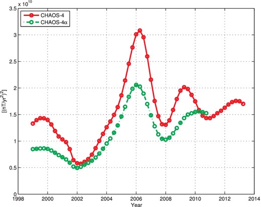
Time variation of the squared field acceleration power (up to degree 8) at the core surface.
4.3 Magnetospheric field contribution
The model coefficients describing the magnetospheric part of CHAOS-4 (cf. eqs 4 and 5) are listed in Table 2. |$\overline{\Delta q_1^0}=1.90$| nT, the mean value of the external axial dipole terms |$\Delta q_1^0(t)$| in the SM frame averaged over the 900 5-d bins, is much smaller than the corresponding term |$q_1^{0,{\rm GSM}}=11.89$| nT in the GSM frame. If RC exactly described the magnetic field contribution in the SM frame as seen by the satellites Ørsted, CHAMP and SAC-C one would expect a vanishing ‘baseline correction’ |$\Delta q_1^0$| and a regression coefficient |$\hat{q}_1^0=-1$|; the estimated values (|$\overline{\Delta q_1^0}=1.90$| nT, |$\hat{q}_1^0=-0.91$|) indicate that RC provides a rather good description of the SM magnetic field contribution at satellite altitude. However, although |$\hat{q}_1^0$| is close to −1 it is nevertheless smaller (in absolute value) than the expected value. This means that the time changes of the SM magnetospheric field as seen by the satellites are only 91 per cent of that predicted by RC as derived from ground data. Nonetheless, this value is closer to −1 than was the case for previous estimates using Dst instead of RC to describe the magnetospheric field contributions.
Model coefficients of the magnetospheric part of CHAOS-4. For details see Section 4.3.
| |$\overline{\Delta q_1^0}$| | = | 1.90 nT | |$\hat{q}_1^0$| | = | –0.91 |
| |$\overline{\Delta q_1^1}$| | = | –1.05 nT | |$\hat{q}_1^1$| | = | –0.01 |
| |$\overline{\Delta s_1^1}$| | = | –0.17 nT | |$\hat{s}_1^1$| | = | –0.01 |
| |$q_2^0$| | = | –1.06 nT | |$q_1^{0,{\rm GSM}}$| | = | 11.89 nT |
| |$q_2^1$| | = | –1.78 nT | |$q_2^{0,{\rm GSM}}$| | = | 1.43 nT |
| |$s_2^1$| | = | 0.81 nT | |||
| |$q_2^2$| | = | –0.58 nT | |||
| |$s_2^2$| | = | 0.07 nT |
We also derived a model similar to CHAOS-4l but using Dst(t) = Est(t) + Ist(t) instead of RC(t) = ϵ(t) + ι(t). The estimated regression coefficient of that model is |$\hat{q}_1^0=-0.84$|, which means that the SM field seen by the satellites is only 84 per cent of the one predicted by Dst. Perhaps even more important is the ‘baseline correction’ |$\Delta q_1^0(t)$| of that model, shown by the red dots in Fig. 12. The values scatter considerably more (rms = 6.7 nT) compared to the ones derived using RC (blue dots, rms = 2.8 nT). This is indicative of the baseline-instabilities of the Dst-index, as is also obvious when looking at the difference between the external parts of Dst and RC (black curve of Fig. 12). All these findings indicate that RC provides an improved description of the magnetospheric field (in particular during quiet conditions) compared to Dst.
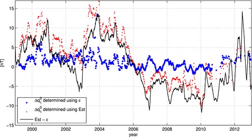
External field ‘baseline corrections’ |$\Delta q_1^0$| in dependence on time for CHAOS-4 (blue dots). Values from a similar model run parametrized by Dst instead of RC are shown in red. The difference ϵ(t) − Est(t) between the external parts of RC and Dst is shown by the black curve. All values are 30-d running means (see Section 4.3).
The non-axial dipole external field coefficients (|$q_1^1,s_1^1$|) of CHAOS-4 are uncorrelated with RC, as can be seen from the vanishing regression coefficients |$\hat{q}_1^1, \hat{s}_1^1$|. The mean values |$\overline{\Delta q_1^1}=-1.05$| nT, |$\overline{\Delta s_1^1}= -0.17$| nT of the corresponding ‘baseline corrections’ are also close to zero, and their rms scatter around the mean is below 1 nT. This indicates that the dipole-part of the magnetospheric field can be well described by the RC index plus the field of a degree-one zonal coefficient in the GSM frame of amplitude ≈12 nT. For comparison Lühr & Maus (2010) reported for the scaling factor |$\hat{q}_1^0=-0.87$| and the stable GSM field |$q_1^{0,{\rm GSM}}=8.31$| nT.
Let us finally discuss the remaining non-dipole external field terms: The largest magnetospheric coefficient (apart from |$q_1^{0,{\rm GSM}}$|) is |$q_2^1 = -1.78$| nT. Together with the corresponding coefficient |$s_2^1 = +0.81$| nT it produces a diurnal magnetic field variation of strength 1.9 nT with maximum (negative) amplitude at 22:20 MLT. Although this value has been derived from nightside data only it is in good agreement with the prediction of the Tsyganenko model (e.g. Tsyganenko 1990). Olsen (1996) found a contribution to the degree-2 order-1 spherical harmonic coefficients for geomagnetic quiet conditions (Kp = 0) of strength 1.4 nT with maximum (negative) amplitude at 23:48 MLT.
5 CONCLUSIONS
Using more than 14 yr of continuous satellite data, augmented with revised monthly means from magnetic observatories, we have derived a model of the static and time-varying part of the Earth's magnetic field. The model describes rapid core field variations occurring over only a few months as well as the lithospheric field at least up to spherical-harmonic degree n = 85.
Data from the Swarm satellites launched in November 2013 will make it possible to extend the CHAOS model series both regarding better resolution of small-scale lithospheric field features and more rapid time changes of the core field. Processing, calibration and validation of the Swarm data during the first months of the mission lifetime requires an accurate reference model of the geomagnetic field which we believe CHAOS-4 can provide. However, one has to be careful when extrapolating CHAOS-4 to times beyond the data span period (1997.5–2013.5). In addition, some model coefficients describing the core field after mid-2010 might be affected by the Backus effect since only scalar satellite data have been used after 2010 September. This mainly concerns sectorial terms |$g_n^n, h_n^ n$|. Inclusion of vector data from Swarm will mitigate these problems. We plan to update CHAOS-4 by augmenting with Swarm data as soon as these data become available.
Previous versions of CHAOS and the data used for their determination have been widely used for scientific studies, and we hope that CHAOS-4 will also prove useful to the scientific community, both regarding investigations of the dynamics of the core field, the detailed structures of the lithospheric field and in unravelling the various magnetospheric contributions.
Model coefficients of CHAOS-4 and data sets used for their determination are available in different formats at www.spacecenter.dk/files/magnetic-models/CHAOS-4/.
This paper has been finalised while N.O. was visiting Professor at University of Edinburgh, kindly supported by The Leverhulme Trust. We would like to thank the staff of the geomagnetic observatories and INTERMAGNET for supplying high-quality observatory data, and Susan Macmillan for providing us with checked and corrected observatory hourly mean values. The support of the CHAMP mission by the German Aerospace Center (DLR) and the Federal Ministry of Education and Research is gratefully acknowledged. The Ørsted Project was made possible by extensive support from the Danish Government, NASA, ESA, CNES, DARA and the Thomas B. Thriges Foundation.
