


Abstract
Marine seismology usually relies on temporary deployments of stand alone seismic ocean bottom stations (OBS), which are initialized and synchronized on ship before deployment and re-synchronized and stopped on ship after recovery several months later. In between, the recorder clocks may drift and float at unknown rates. If the clock drifts are large or not linear and cannot be corrected for, seismological applications will be limited to methods not requiring precise common timing. Therefore, for example, array seismological methods, which need very accurate timing between individual stations, would not be applicable for such deployments.
We use an OBS test-array of 12 stations and 75 km aperture, deployed for 10 months in the deep sea (4.5–5.5 km) of the mid-eastern Atlantic. The experiment was designed to analyse the potential of broad-band array seismology at the seafloor. After recovery, we identified some stations which either show unusual large clock drifts and/or static time offsets by having a large difference between the internal clock and the GPS-signal (skew).
We test the approach of ambient noise cross-correlation to synchronize clocks of a deep water OBS array with km-scale interstation distances. We show that small drift rates and static time offsets can be resolved on vertical components with a standard technique. Larger clock drifts (several seconds per day) can only be accurately recovered if time windows of one input trace are shifted according to the expected drift between a station pair before the cross-correlation. We validate that the drifts extracted from the seismometer data are linear to first order. The same is valid for most of the hydrophones. Moreover, we were able to determine the clock drift at a station where no skew could be measured. Furthermore, we find that instable apparent drift rates at some hydrophones, which are uncorrelated to the seismometer drift recorded at the same digitizer, indicate a malfunction of the hydrophone.
1 INTRODUCTION
Within the DOCTAR project (Deep OCean Test ARray), we examine the potential of broad-band array methods on the ocean floor. The application of array methods requires a synchronized network (Rost & Thomas 2002). On shore, this is usually achieved by continuous clock synchronization with a GPS signal. In the deep sea, GPS signals cannot be recorded. Therefore, clock synchronization can only be achieved before deployment and after recovery of the stations (e.g. Geissler et al.2010). The measured time difference between the data logger and GPS after recovery is referred to as skew. Several studies deal with clock drift measurements and synchronization of seismic on-shore networks using ambient noise cross-correlation (Stehly et al.2007; Sens-Schönfelder 2008). The advantage of such methods, beside the low cost aspect, is that they can be applied off-line a posteriori to correct data already recorded.
Up to our knowledge, there has only been one successful application of synchronization using ambient noise cross-correlation at an ocean bottom station (OBS) installation, which was at shallow water depth (several tens of metres) and several metre interstation distances (Sabra et al.2005).
In this study, we demonstrate the feasibility of ambient noise clock synchronization for deep water depths and km-scale installations. Such network geometries require long correlation times (at least 1 d) to achieve good signal-to-noise ratios (SNRs) and stable correlation results. We further extend the standard method to identify static time offsets and large clock drifts, which are present at some stations of our OBS deployment. The method demonstrated here is useful to estimate the parameters for the correction of time drifts and offsets, which is a first step to greatly improve the relevance of OBS network data.
2 DATA
In 2011, twelve free-fall OBS (DEPAS pool, http://www.awi.de/en/go/depas) were deployed in the 4.5- to 5.5-km-deep water of the mid-eastern Atlantic, north of the Gloria Fault, 800 km off the coast of Portugal. Each station consists of a broad-band seismometer (Guralp CMG-40T, 60 s-50 Hz) and a hydrophone (HighTechInc HTI-04-PCA/ULF, 100 s-8 kHz, flat instrument response down to 5 s, at D08 down to 2 s). The sensors share the same data logger [Send Geolon MCS, 24 bit, 1–1000 Hz, 20 GB; see Dahm et al. (2002) for detailed instrument description]. The stations formed an array with an aperture of approximately 75 km (see Fig. 1).
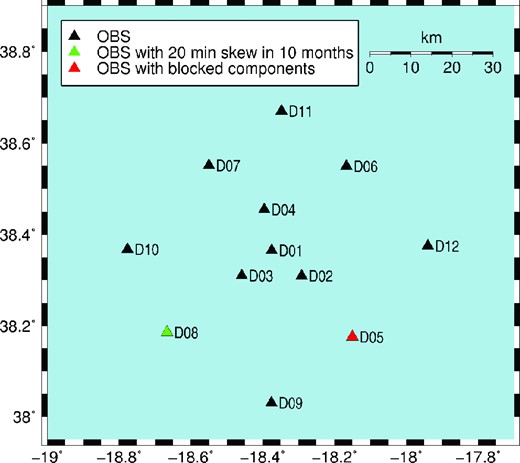
Configuration of OBS deployment.
The stations recorded from 2011 July until 2012 April with a sampling rate of 100 Hz. During recovery, we identified three stations with problems concerning the timing. For station D05, no skew measurement was possible. The recording at this station stopped 1 month before the recovery, possibly due to a higher energy consumption because of a clamped vertical and one clamped horizontal component, meaning that these components were at their maximum values (see Fig. 2a, D05 Z). Furthermore, station D08 and D09 show unusually high skews of around 20 min and 10 s (Fig. 1 and Table 1). All other stations had ‘normal’ skews smaller than 1.5 s (Table 1).
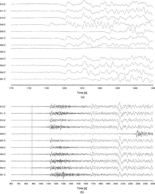
Examples for teleseismic events, unfiltered data. 0 s corresponds to origin time in each case, station D05 has only data for the first event because of the power loss 1 month before the recovery, red line in (b) shows time of maximum of P wave for all stations except for D08 and D09, Mw is the moment magnitude, Δ the distance in degree and Φ is the azimuth of the event seen from station D01 (Δ and Φ estimated from location of USGS (http://earthquake.usgs.gov/earthquakes/eqarchives/epic/, last accessed 30 October 2013), the slowness values were taken from the AK135 TravelTime Tables (http://rses.anu.edu.au/seismology/ak135/intro.html, last accessed 30 October 2013): (a) 06.07.2011 19:03:18.26, Mw = 7.6, depth = 17 km, Δ = 159.72°, Φ = 289.23°; phase PKPdf (PKIKP) with slowness 1.18 s degrees−1; (b) 11.04.2012 08:38:37.36, Mw = 8.6, depth = 22 km, Δ = 105.22°, Φ = 74.52°; phase P with slowness 4.45 s degrees−1.
Skew measurements tskew after recovery and nominal clock drift Δd per year assuming a linear drift.
| Station | tskew (s) | Δd (s a−1) |
|---|---|---|
| D01 | 0.260812 | 0.319 |
| D02 | 1.337781 | 1.638 |
| D03 | 0.415937 | 0.510 |
| D04 | 0.504531 | 0.615 |
| D05 | — | — |
| D06 | −0.038125 | −0.047 |
| D07 | 0.377656 | 0.462 |
| D08 | 1201.108843 | 1472.38 |
| D09 | −8.36275 | −10.318 |
| D10 | 0.520906 | 0.640 |
| D11 | 0.928687 | 1.138 |
| D12 | 0.0095 | 0.012 |
We checked the relative timing between stations with strong teleseismic events (Fig. 2) by performing a beam for the first arrival [compare captions in Fig. 2 for details and Rost & Thomas (2002) for method]. We choose one event shortly after the deployment (2011 July 6, Fig. 2a) and another slightly before the recovery (2012 April11, Fig. 2b). Thus, we could verify that D08 shows indeed an extremely high clock drift as indicated by the measured skew of 20 min. Furthermore, we note that the 10 s skew at D09 seems to be related to a time offset which is constant over the whole period of the experiment, since the time offset was already present shortly after the beginning of the experiment (Fig. 2a and time difference shown by red line in Fig. 2b). We checked the log-files of the recorders and find that the first synchronization (during deployment) was not logged in the file of station D09 as it was in case of all other stations. This seems to indicate that the first synchronization has failed at station D09. Besides this, the station worked normally.
3 THEORY
In this section, we consider some simple examples to make clear which influence a linear clock drift has on correlation results. These examples deal with separated, undisturbed signals, but the effects are similar for ambient noise cross-correlations where several signals from different directions and sources are superimposed (Stehly et al.2007; Sens-Schönfelder 2008).
Herein, f1 is the signal measured at sensor 1 and f2 the signal measured at sensor 2, τ is the lag-time.
Therefore, the correlation result is a delta impulse located at the lag-time which corresponds to the negative traveltime between sensor 1 and 2, which is equivalent to the lag-time of the correlation of unskewed signals, delayed by the time that corresponds to the influence of the static time offset tc and the relative clock drift δd between the sensors on the arrival time of the signal at sensor 2.
A synthetic example should demonstrate, how a clock drift influences the correlation results in consecutive time windows and how it can be measured. We consider a more complex signal at sensors 1 and 2 which consists of several short wavelets which occur every 20 s starting at 5 s at sensor 1 and at 10 s at sensor 2 (Fig. 3, black solid lines traces 1 and 2). Furthermore, we assume a skewed signal with a clock drift of 1 s per 100 s at sensor 2 (Fig. 3, red dashed line trace 2). We introduce common, unshifted time windows to cut out traces before applying the cross-correlation (blue boxes in Fig. 3). The resulting cross-correlation function for each time window are also presented in Fig. 3 (black solid line = unaffected by a clock drift and red dashed line = influenced by the effect of the clock drift).
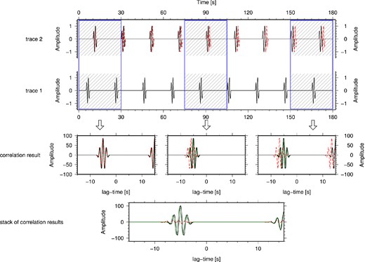
Synthetic example to visualize the effect of the clock drift, black solid lines are unskewed data and their correlation results, red dashed line is for skewed data, blue box shows used time window, green solid line gives correlation result from shifted time windows (grey shading).
We observe that the influence of the clock drift increases for later time windows. From eq. (4), we know that the time difference between the correlation without clock drift and the one with clock drift corresponds to the influence of the static time offset and the clock drift on the arrival times of the signal at sensor 2. This effect is linear in δd and visible in the synthetic example, too. Therefore, we can estimate the clock drift by comparing the correlation of the first time window with the correlation results of all consecutive time windows. On the other hand, this example illustrates that the stack of correlation traces of consecutive time windows affected by a clock drift would lead to a correlation trace with a more or less smeared signal depending on the amount of the clock drift [see stacks of correlation results in Fig. 3, compare black solid (without skew) and red dotted line (with skew)]. We would expect that we will not get any usable correlation signal for large clock drifts (several seconds per day), because either they lead to time differences which could be larger than the chosen correlation time window or even if the window was properly set, the clock drifts would cause a strong smearing.
The grey shading in Fig. 3 shows the shifted time windows in case of the synthetic example. The green solid lines represent the resulting cross-correlation functions for the shifted time windows. We observe that they are only influenced by the clock drift within the short time windows and that their difference in lag-time does not increase for later time windows. By comparing the stack of the unskewed and the shifted time window correlation results (see lower panel in Fig. 3, green and black solid lines), we find that the signal is nearly identical except for a small difference in amplitude and lag-time, which represents the influence of the clock drift in the short time window.
If we deal with a data set where all signals are skewed, we only can estimate relative clock drifts between the sensor pairs. We need additional information such as skew measurements or stations with continuous GPS synchronization to get an absolute timing. Therefore, the stations of a network, where no additional information concerning the timing is available, can only be synchronized relatively to one reference station.
4 METHOD
4.1 Estimation of clock drifts
Herein, |$t_{diff_0}$| is the clock difference at T0 = 0. This parameter is also estimated by the linear regression and should be close to zero.
If we compare the relative clock difference after 1 yr calculated by the results of the regression with the expected values estimated from the measured skews, we can determine all parameters needed for the timing correction of the data set.
4.2 Constant time-shifts
Herein, tm is the estimated clock difference from the correlations which reflects the influence of the actual clock drift δd over the length Tcorr of the used time window. The time tth is the expected time difference for the used time window calculated with the apparent clock drift δdapp which results from the measured skews and the time T between synchronization and skew measurement by neglecting the effect of the static time offset tc.
4.3 Shifted correlation time window approach
For station D08, we know from the measured skew (compare Table 1) that the overall clock drift is around 20 min for 10 months of recording, which is coarsely validated by the beam forming (Fig. 2). We use shifted correlation time windows (see eq. 5) to estimate the clock drift at station D08 for the vertical seismic component. Hereby, the drift rates of all other stations remain unchanged and are assumed to be constant.
If the tested skew, which is used to calculate the expected clock difference by assuming a linear clock drift, is correctly chosen, the lag-time of the resulting cross-correlation will only be influenced by the clock drift in the chosen correlation time window. The method of the shifted correlation time windows offers the opportunity to systematically test for several clock drifts. This might be useful in case of no, lost or erroneous skew measurements. After performing several tests with different skews and therefore clock drifts, all correlations from the whole available recording period are stacked for each assumed clock drift and the maximum amplitudes of the resulting traces are estimated as a quality measure. The tested value which belongs to the highest maximum amplitude is assumed to be the most likely (compare stacks of correlation results in synthetic example Fig. 3).
4.4 Processing of data set
We decide to cross-correlate the vertical seismic components of our whole data set day by day. The processing is similar for the unshifted and the shifted time windows except for some details. The day traces are split into 90 s windows which overlap by 50 per cent on which we perform the cross-correlation. The window length was chosen because of the largest interstation distance of 75 km and an assumed surface wave velocity of 2 km s−1. The latter results from the assumption of a very thin sediment layer which is based on the observation of the high-frequency content (up to 30–40 Hz) of local events and the steep incidence angles of teleseismic events. In contrast to the unshifted time windows, we have to check whether the shifted correlation time window for the second input trace is still within the time range of the chosen trace time window, which is in our case 1 d. The resulting correlation traces of the different time windows are stacked. The stacked correlation result with unshifted time windows corresponds to the correlation result for the whole trace (Bensen et al.2007), although it is now probably influenced by the relative clock drift between the stations. We estimate the correlation traces from −40 to 40 s lag-time which should be sufficient for Rayleigh-wave propagation between the stations of the array.
Furthermore, we also correlate the hydrophone signals. There, we choose 180 s time windows with 50 per cent overlap and estimate the correlations from −60 to 60 s lag-time. The larger time window is necessary because of the acoustic velocities which are slower than the seismic ones. We perform the correlations of the hydrophone signals to test whether they show the same behaviour as the seismic components.
For the pre-processing of the data, we mainly follow the work by Bensen et al. (2007) and Picozzi et al. (2009). We use the one-bit and spectral normalization and remove the global and the local offset. Furthermore, we stack the correlation traces of 20 consecutive days (here referred to as 20 d stack) every 5 d to increase the SNR of the correlation trace. We apply a low-pass filter with a corner frequency of 1 Hz before estimating clock differences from the 1 d and the 20 d stack. For better comparison, we determine the amount of clock difference after 1 year.
5 DISCUSSION
5.1 Correlation of vertical seismic components
In Fig. 4, the correlation result (20 d stack) for the vertical seismic components of the station pair D01 and D02 is presented as an example. The correlation signal is asymmetric which is related to a non-isotropic distribution of noise sources (Stehly et al.2006). The different amplitudes over time might be related to changes in the strength and distribution of the noise sources. We observe a linear shift of the correlation signal with time (Fig. 4) which reflects the influence of a relative clock drift between the stations. For the estimation of the time-shifts, we used a cross-correlation of the first correlation trace and all consecutive traces without any normalization, any tapering or any offset removal. The used time windows were 5 s long and had an overlap of 50 per cent. We also tested longer time windows of 15 and 40 s which gave similar results. By plotting the estimated clock differences against the starting day of the time windows used for the stack (Fig. 5), we can validate the linear drift as expected by eq. (4). Moreover, we are able to use a linear regression to estimate the clock drift per second and calculate from this the clock difference which would be present after 1 yr of recording.
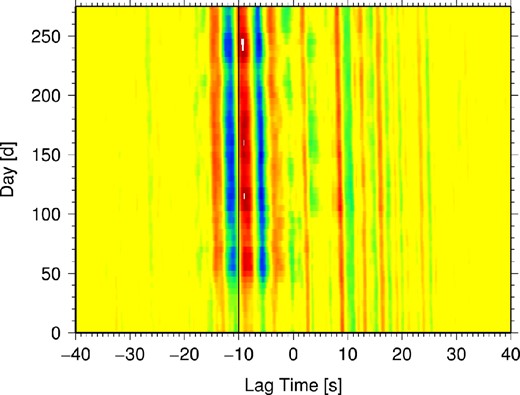
Amplitude of stacked correlation traces (20 d stack) over lag-time and starting day of the vertical seismic components of stations D01 and D02, the amplitude is normalized to the maximum of all correlation traces. The black line is given as a reference.
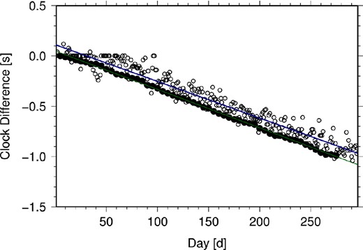
Comparison of the clock differences estimated from 1 d (open circles) and 20 d stacks (filled circles) of the vertical seismic components for station pair D01 and D02. The blue and the green line show the trend lines resulting from linear regression.
We observe in Fig. 5 that the results from the 20 d stacks (filled circle) have smaller deviations compared to the trend line than the ones estimated from the 1 d correlations (open circles). This is related to the better SNR of the 20 d stacks. Therefore, we will use the results from the 20 d stack for the following discussion. We made a comparison of the results for the vertical seismic components for all station pairs with the expected clock differences (Fig. 6). The errors were estimated by using eq. (6).
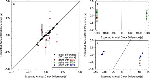
Comparison of the estimated annual clock differences of 20 d stacks of the correlations of the vertical seismic components with expected values from skew measurements. The error bars give the value of |$\sigma _{t_m}$| as defined in eq. (6). Station pairs involving D05 are plotted red, D08 green and D09 blue, the lines indicate where estimated and expected values are equal.
Herein, |$t_{m_i}$| is the estimated annual clock difference from the clock drift per second which was estimated by the correlations of the i-th station pair. The value |$t_{{\rm th}_i}$| is the expected annual clock difference from the skew measurements of the i-th station pair.
We obtain two groups in Fig. 6(b) and (c) which have large differences between the estimated and the expected annual clock differences. By identifying the related station pairs, we find that the group with expected values around 1500 s and large errors always includes station pairs involving D08 (Table 1 and Fig. 6b, green symbols). This result and the corresponding correlations without any usable signal (not presented here) show that the estimation of large clock drifts is not possible with ambient noise cross-correlation by using unshifted correlation time windows.
On the contrary, the estimated annual clock differences for the group with the expected values around 10 s and small errors (blue symbols in Fig. 6c) indicate a small linear drift for the vertical seismic component. We find that all station pairs within this group include the station D09 (blue symbols in Fig. 6). Therefore, we confirm our observation from the beam forming (Fig. 2) that this station has a static time offset. Moreover, we can estimate this time offset from our observation and in addition correct the skew for the timing correction of the data (Table 2). To determine the static time offset, we used eq. (9) for the values of all station pairs involving station D09 and calculated afterwards the mean of the resulting time offsets. This leads to a static time offset of −9.213 ± 0.009 s (compare Table 2) and a corrected annual drift rate of 1.049 s a−1 for station D09.
Annual clock differences for station D09 as reference station, tm is the estimated annual clock difference from the 20 d stacks for the vertical seismic component (the error is estimated by using eq. 6) and tth is the expected annual clock difference calculated from the measured skews, tc is the constant time-shift calculated according to eq. (9).
| OBS | tm (s) | tth (s) | tc (s) |
|---|---|---|---|
| D01 | 0.752 ± 0.032 | −10.638 | −9.231 ± 0.026 |
| D02 | −0.542 ± 0.018 | −11.957 | −9.252 ± 0.015 |
| D03 | 0.550 ± 0.024 | −10.828 | −9.222 ± 0.020 |
| D04 | 0.483 ± 0.027 | −10.934 | −9.253 ± 0.022 |
| D06 | 1.168 ± 0.040 | −10.272 | −9.271 ± 0.033 |
| D07 | 0.502 ± 0.039 | −10.781 | −9.144 ± 0.031 |
| D10 | 0.216 ± 0.036 | −10.959 | −9.057 ± 0.029 |
| D11 | −0.020 ± 0.028 | −11.457 | −9.269 ± 0.023 |
| D12 | 1.041 ± 0.051 | −10.330 | −9.216 ± 0.042 |
| Mean tc (s) | −9.213 ± 0.009 | ||
| Measured skew (see Table 1; s) | −8.36275 | ||
| New skew corrected with tc (s) | 0.850(25) | ||
| New clock drift per year Δd (s a−1) | 1.049 | ||
Additionally, we observe in Fig. 6 that the estimated values for station pairs involving D05 (red symbols) show random deviations from the ‘ideal’ line and large errors. This effect was expected because of the clamped vertical seismic component as has been mentioned before. Consequently, we are not able to obtain any information for the timing correction from the correlations of vertical seismic components and exclude the vertical seismic component of D05 from further investigations concerning the vertical seismic components.
5.2 Shifted correlation time window approach
For the test of the shifted correlation time window approach, we present the resulting maximum amplitudes of the stacks for the whole recording period over the tested annual clock drifts for station D08 in Fig. 7. The highest value for the maximum amplitude of the stacked correlations is reached for the annual clock drifts of 1472.24 s a−1 and 1472.86 s a−1. The value estimated by the measured skew lies at 1472.38 s a−1 (compare Table 1 and grey line in Fig. 7) which is just in-between the two most likely test values. Therefore, the shifted correlation time window approach and the selected quality criteria are feasible for the testing of large clock drifts. Furthermore, we observe that the value of the maximum amplitude is partly related to the distance between the stations, although it is not direct proportional. Additionally, we took the corrected annual clock drift for station D09 for the calculation of the new start of the correlation time window on the second input trace which gives the highest maximum amplitude for an annual clock drift of 1472.24 s a−1. This observation confirms that the correction for the static time offset at station D09 was successful.
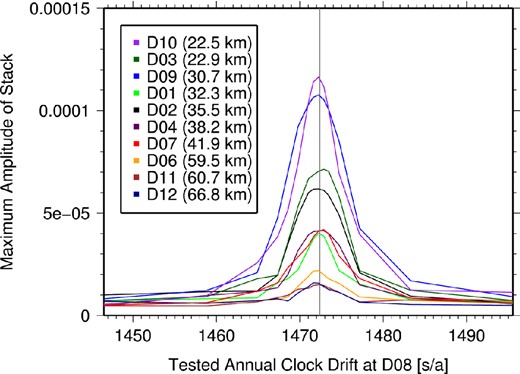
Maximum amplitude of the stack of all correlation traces (i.e. for the whole recording period) for different annual clock drifts tested and stations in combination with station D08, the distance to station D08 is given in braces. The tested annual clock drifts are equivalent to the value in the third column of Table 1, the grey line indicates the annual clock drift for D08 as can be calculated by the measured skew.
5.3 Correlation of hydrophone signals
Hydrophone and seismometer share the same data logger, therefore we expect to observe a similar drift behaviour and similar drift rates from the correlations of the hydrophone signals as from the correlations of the vertical seismic components. Moreover, we hope to extract an information about the drift rate of station D05 where the vertical seismic component was clamped, but the hydrophone was working.
Careful data inspection showed that the hydrophones show a malfunction at two stations (D02 and D12) at the beginning of the recording and that the hydrophone at D03 shows data errors for most of the recording period. The stations D02 and D03 show quite small amplitudes and all three stations have steps in the amplitude which sometimes slowly recover during periods of malfunction.
If we have a look at the correlation results of the remaining stations, we find that they show a good agreement in the clock drift behaviour between seismometer and hydrophone. The standard deviation of the difference between the estimated clock differences and the expected values is ±0.129 s for the hydrophone signals (calculated with eq. 10). This is slightly larger than the standard deviation of the differences for results of the vertical seismic components (±0.087 s).
Furthermore, we are able to give a rough estimate for the annual clock drift at station D05 of 0.775 ± 0.012 s a−1 by comparing the estimated and the expected annual clock differences for all hydrophones with constant drift rates (Table 3).
Annual clock differences for station D05 as reference station, tm is the estimated annual clock difference from the 20 d stacks for the hydrophone signals (the error is estimated by using eq. 6) and tth is the expected annual clock difference calculated from the measured skews, tdiff gives the differences between estimated and expected clock difference.
| OBS | tm (s) | tth (s) | tdiff (s) |
|---|---|---|---|
| D01 | 0.434 ± 0.024 | −0.319 | 0.753 ± 0.024 |
| D04 | 0.264 ± 0.018 | −0.615 | 0.880 ± 0.018 |
| D06 | 0.652 ± 0.040 | 0.047 | 0.606 ± 0.040 |
| D07 | 0.277 ± 0.024 | −0.462 | 0.740 ± 0.024 |
| D09 | −0.018 ± 0.007 | −1.049 | 1.031 ± 0.007 |
| D10 | 0.069 ± 0.047 | −0.640 | 0.709 ± 0.047 |
| D11 | −0.433 ± 0.047 | −1.138 | 0.705 ± 0.047 |
| Mean tdiff (s) | 0.775 ± 0.012 | ||
The partly malfunction of the hydrophones at station D02 and D12 is reflected by the estimation of instable apparent drift rates for station pairs involving these stations in the periods of the malfunction (compare Fig. 8 first 100 d). Besides this period, the extracted clock differences show a clock drift which is similar to the clock drift estimated by the correlation of the vertical seismic data (Fig. 8). The nearly total malfunction of the hydrophone at station D03 leads to a complete vanishing of any signal in the correlation results after 200 d of recording (mid of 2012 January).
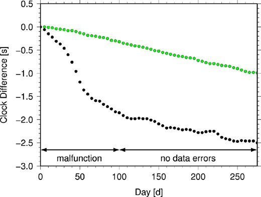
Comparison of the clock differences estimated from 20 d stacks of the vertical seismic components (green) and hydrophone signals (black) of station pair D01 and D02. The arrows indicate the period of malfunction and when no data errors occurred.
6 CONCLUSION AND OUTLOOK
In summary, we find that the linear clock drift is visible in the correlation results of the vertical seismic components and that relative annual clock differences can be estimated except for station pairs involving D05, which had a clamped vertical seismic component. Furthermore, the comparison with expected annual clock differences determined by the measured skews and the assumption of a linear drift shows a good agreement (standard deviation of differences is ±0.087 s). Additionally, we calculate the amount of a static time offset at station D09. Moreover, we prove that the shifted correlation time window approach gives usable results for station D08 which had a large clock drift and can be applied to test for a range of clock drifts to find the most likely. It should be mentioned that the verification of the clock drift with events might be helpful, but it is not required. So even in the case of short-term deployments where no or only few large earthquakes occur within the recording period, the application of ambient noise cross-correlation for clock drift estimations is possible as long as the time period of the recording is sufficient to get a stable correlation result with a sufficient SNR for several consecutive time windows.
Furthermore, we find that the linear clock drift is also visible for most of the hydrophones (standard deviation of differences is ±0.129 s). We were able to estimate an annual drift rate for station D05 which had a clamped vertical seismic component by using the correlation results of the hydrophone signals. Furthermore, we find that instable drift rates at some hydrophones indicate periods of malfunction at these sensors.
Another possibility to estimate drift rates of instruments with clamped vertical seismic components might be the correlation of the horizontal components, although it is not clear whether and to which degree orientation, which is usually unknown for free-fall OBS stations, is important for this purpose. Besides, a test-wise rotation of the horizontal components of one station with known orientation might offer an additional information about the orientation of the horizontal components of the other stations. Preliminary tests give promising results, but need further investigations concerning orientation-dependent quality measures.
It should be mentioned that the processing of ambient noise cross-correlation highly depends on the noise field, noise source distribution and strength, the structure beneath the stations, interstation distances and recording length (for further details concerning the processing of ambient noise cross-correlation see Bensen et al.2007). To determine optimal processing options, we examined the pseudo-shot gather of the cross-correlation functions of all stations, whether a propagating wave front is clearly visible and furthermore, we had a look at the stability of the cross-correlation results within the consecutive time windows used for the analysis.
Finally, we conclude that ambient noise cross-correlation is one feasible method to check the timing and synchronization of deep water, km-scale OBS arrays. It also can be applied off-line a posteriori to correct data already recorded. The method works well for vertical seismic components, but needs further investigations in case of hydrophone signals and horizontal components.
The authors want to thank the DEPAS pool for providing the instruments for the DOCTAR project which is funded by the DFG. The examination of the data was done using Seismic Handler (Stammler 1993). All figures were created using GMT [Generic Mapping Tools, Wessel & Smith (1991)].
