


Abstract
The appearance of clay in fractures is an important issue of applied geoscience as it not only affects the stability but also the flow paths through rocks. Forming a link between hydraulic, geochemical and mechanical processes, clay structures need to be thoroughly investigated. The growing importance of clay for waste disposal, petroleum research, geothermal exploration and geotechnical engineering necessitates tools to find and to characterize clay structures and clay minerals indirectly from geophysical measuring methods. Particularly, there is need for a technique enabling to map clay-rich zones from geophysical well logs acquired on-site in order to assess the mechanical and hydraulic properties of rocks. In this study, we present a neural network based method to map clay bearing fracture zones in crystalline facies. The study has been performed on the basis of geophysical and geological data acquired at the geothermal site of Soultz-sous-Forêts (France), in the granitic reservoir. A neural network was trained on geophysical logs from the fully cored exploration well EPS1. Calibration of the network was done on reference logs derived from the drill core. The effective calibration enabled the creation of synthetic clay content logs, which predict the clay amount in fractures along the well with >74 per cent accordance with a reference log.
High clay contents could be located in faults, on which aseismic movements have been identified. The validation of this relationship destines the synthetic logs to help identifying potentially weak zones from geophysical logging methods. With application on non-cored wells, this tool can become a powerful means for assessing the probability of aseismic movements on faults caused by the presence of clay and estimating the hydraulic properties of fractures.
1 INTRODUCTION
1.1 The importance of clay in applied geosciences
Clay bearing structures are of major importance in applied geoscience. A peculiarity of the material is the linkage between geomechanical, hydraulic and geochemical processes. In terms of geomechanics, clay is both a blessing and a curse. Commonly, clay structures in sedimentary rock are of major interest for the safe storage of waste deposits (e.g. Cho et al.2010). Due to its flexible structure, clay can enclose dumped material and seal it from the environment. Therefore, clay formations are regarded particularly suitable for nuclear waste disposal. Contrary, the soft behaviour of clay can be problematic, if its appearance lowers the structural stability of reservoirs, boreholes, slopes or fundaments (e.g. Cappa & Rutqvist 2012; Koleini et al.2012; Mokni et al.2012).
However, clay does not only appear as a sedimentary rock structure, but it also plays a major role as a geochemical alteration product of certain minerals. As such, it appears, for example, in fractured rock, where the appearance of clay minerals on fracture surfaces can hamper the migration of fluids along flow paths (e.g. Velde 1977). As clay plays an important role as a host rock for oil and gas as well as for the migration and retention of hydrocarbons, especially the hydrocarbon industry has put major efforts into the investigation of clay minerals and structures and into techniques for their localization (e.g. Titov et al.2010). Clay mineral identification and localization requires a large variety of geophysical and laboratory methods. As such, geophysical borehole logging is broadly applied using radiometric or electric methods like resistivity logs or induced polarization, neutron scattering and gamma ray logs. Due to their clear signature on K, Th and U logs, clay is often used for stratigraphic correlation in sedimentary rocks, but the complexity of crystalline rocks requires new methods of clay identification and location in the subsurface. This paper focuses the importance of clay for crystalline geothermal systems.
1.2 Clay in crystalline geothermal reservoir rocks
The heat stored in the crystalline basement rock is considered to be the major geothermal resource in wide areas (Kohl et al.2005). Faults and fractured systems in crystalline rocks present hydraulic pathways for hydrothermal fluids. Enhanced Geothermal Systems target fractures to efficiently produce and inject geothermal brine. Because of their high permeability and heat supply, fractured crystalline settings provide ideal conditions for their exploitation as geothermal reservoirs and the production of heat and electricity (e.g. Genter et al.2003).
For EGS both, the presence of hydraulic pathways and the mechanical behaviour of a reservoir are of major importance for the success of hydraulic stimulation and the operation of a power plant. The permeability of a reservoir is one of the limiting factors to the production and injection flow rates. Permeability is not only affected by the dimension and geometry of the fracture, but also by its surface and its filling. The appearance of fractures filled with clay minerals remarkably decreases the permeability of a geothermal reservoir. The hydraulic properties of a fracture play also an important role for the appearance of large earthquakes during hydraulic stimulation (Charléty et al.2007).
‘Fracture’ is a generic term describing a natural discontinuity without visible displacement. It corresponds generally to small-scale discontinuities. At Soultz, many individual fractures were observed and measured from the cores of the EPS1 well (e.g. Genter & Traineau 1992, 1996) in which we conducted our study. They analysed 800 m length of granitic cores and a full structural characterization was conducted. On core, small-scale fractures were systematically filled by carbonates, chlorite, iron oxides, epidote or sulphides mainly. Fractures are mode 1 (opening) fractures. The term fault defines a natural discontinuity with a significant offset. On the cores, it was possible to identify faults due to the occurrence of striations, offset or other structural criteria (Genter & Traineau 1996). Faults were generally filled by secondary hydrothermal minerals such as geodic quartz, carbonates, barite and clay minerals (illite). Faults are mode 2 (shearing) fractures. The concept of fracture zone is also used in this study. It corresponds to a spatial concentration of both fractures (Mode 1) and faults (Mode 2) visible at core scale associated with a significant hydrothermal alteration and the appearance of clay minerals (Genter et al.2000).
Clay minerals inside fractures are formed during alteration of the reservoir rock fostered by the circulation of geothermal brine throughout the history of the reservoir. In fractures of igneous crustal rocks the dissolution of primary minerals and the crystallization of clay minerals are the most significant and the most common fluid–rock interactions (Meunier 2005). The most common geochemical reactions are the alteration of silicates into dioctahedric illite and smectite or trioctahedral chlorite. There are also other processes observed like the recrystallization of phengite and an illitization of previously formed clay minerals. Along with the prevailing stress field and the structure of a reservoir, these processes are supposed to considerably affect the strength of crystalline rock (Valley & Evans 2006) and thus change its mechanical behaviour. Janecke and Evans (1988) found for example that under certain temperature–pressure–strain rate conditions altered feldspars behave ductile instead of brittle in an altered shear zone in southeastern Arizona. Tembe et al. (2006) tested the mechanical properties of cuttings from the SAFOD (San Andreas Fault Observatory at Depth) borehole in central California. They prepared the samples as artificial gouge on granite/sandstone forcing block containing saw cuts. With triaxial frictional sliding tests a profile of the friction coefficient along the borehole was obtained. Samples containing clay minerals had a considerably smaller friction coefficient than quartzo-feldspathic rocks. As together with the laboratory setup many sample preparation parameters could have affected the measurements, it is questionable, if the obtained data is transferable to in situ scales. Duebendorfer et al. (1998) suggest alteration processes as an origin of aseismic shortening in Southern California. Some other authors also found evidence that the presence of clay in fractures as gouge plays an important role for the occurrence of aseismic movements on fault zones and fractures (e.g. Wu et al.1975; Dolan et al.1995; Schleicher et al.2006b). Due to their major importance for reservoir mechanics and in order to be able to plan effective stimulation while mitigating the risk for large earthquakes, it is desirable to be able to map in a geothermal well potentially weak zones correlated with the appearance of clay minerals.
Present approaches to locate weak zones in a reservoir often use P- and S-wave velocities (e.g. Freund 1992) or electrical tools (e.g. Titov et al.2010). One shortcoming of the seismic approach is the low resolution, which makes it impossible to map clay-zones in the scale of few meters. Moreover, the impedance contrast between fractured crystalline rock and clay-bearing fractures is not large enough to differentiate between them both. The identification of clay from electrical logs is difficult, when (conductive) hydrothermal waters fill the reservoir pores or when Fe- bearing minerals occur in the rock matrix. As a consequence, one must always use several log types for interpretation. Unfortunately, they are not always available. Therefore, the goal is to be able to characterize clay-bearing zones based on standard geophysical data. The evaluation of complex interaction between manifold parameters makes it necessary to find a method, which is able to deal with multidimensional input data, to reduce its dimension and to extract the desired information.
With this study, a characterization of the clay distribution along a borehole using geophysical logging data is performed. We introduce a tool for the detection of clay in wellbores on the basis of various geophysical logging techniques. With the help of a neural network analysis (NNA) applied on radioactive log profiles and fracture density curves, synthetic clay content logs (SCCLs) are created for geothermal wells in Soultz-sous-Forêts (Alsace, France). After a rough review of the available data, reference clay content logs [index-SCCLs (iSCCLs)] are created from core data of the investigation well EPS1. These logs are reference data sets, which represent the real clay content inside faults of the granite derived from core analysis. The neural network is then trained on the logging data of the well based on information from the iSCCL. The network is calibrated and different input parameters are tested in order to find the configurations that yield the best result. Finally, the benefit of this results on the estimation of reservoir hydraulics and geomechanics is discussed.
2 THE GEOTHERMAL SITE IN SOULTZ-SOUS-FORÊTS
2.1 Geology and alteration processes
The geothermal site in Soultz sous Forêts at the western boundary of the Upper Rhine Graben is a multiwell system with the two injection wells reaching a depth of 5100 m (GPK3) and 3600 m (GPK1), respectively and the production well reaching 5080 m (GPK2). Two more wells were drilled to 5260 m (GPK4) and 2230 m (EPS1) depth, respectively. The elaborately investigated pilot well EPS1 will be of major importance for this study.
The reservoir rock is an intrusion of a post-tectonic Variscan monzogranite overlain by a sedimentary cover of 1400 m thickness. The mineralogical composition of the granite is mainly characterized by large K-feldspar megacrysts in a matrix of quartz, biotite, plagioclase and amphibole. Accessory minerals are titanite, apatite and magnetite (Genter & Traineau 1991). During the multiphase tectonic history of the opening of the Upper Rhine Graben a pronounced fracture network formed in the granitic rock. Simultaneously, several stages of fluid inflow can be reconstructed (Schleicher et al.2006a), during which primary minerals have been dissolved and secondary mineral phases precipitated. The earlier propylitic alteration is a weak isochemical alteration of the granitic matrix without a change in the granite texture. It incorporates the partial transformation of biotite and hornblende into chlorite, the replacement of plagioclase by illite and the formation of hydrogarnet and epidote within the granite. The second alteration, superposing the earlier stages involves strong chemical and textural changes mainly in and in the vicinity of fractures. In some altered zones, quartz, biotite, plagioclase and hornblende are totally dissolved (Ledésert et al.2010). The precipitations in veins contain secondary quartz, barite, illite, carbonates, iron oxides and locally illite-smectite and chlorite-smectite mixed-layered minerals (Genter et al.2000; Schleicher et al.2006a).
The fractured zones in the Soultz granite have a specific structure, which can be seen in Fig. 1. Around the quartz vein, which often seals the centre of the fracture, a distinct zonation is observed. In the brecciated and cataclased zone, the original structure of the granite is lost and hydrothermal alteration has transformed feldspars or biotite into clay minerals. Depending on the respective minerals that have formed, the granite becomes greenish in the case of chlorite or epidote, reddish, if hematite has formed or yellowish if the dominating clay mineral is illite (Genter et al.2000). This vein alteration is significantly changing the mechanical and structural properties of the rock. Along with the mineralogy the physical parameters like porosity, bulk density and P-wave velocity of the rock change (Ledésert et al.2010). Valley and Evans (2006) found from laboratory measurements that the uniaxial compressive strength of the granite is lower for samples showing vein alteration. These altered zones are therefore of major interest in terms of rock mechanical properties.
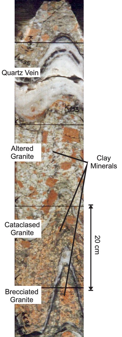
The zonation of an altered fault. Unrolled photograph of the EPS1 core K195, at 2156 m depth (top). The picture represents a scanned core, which means that planar lines become sinusoidal if they cut the core at an angle, which is not horizontal. Clay minerals occur mainly in the zone of hydrothermally altered granite, but they can also occur in the remaining zones. Two consecutive horizontal lines represent 20 cm.
2.2 The Soultz Log database
During many years of scientific research at Soultz, a huge database of logging data, research results and scientific publications has been accumulated for the geothermal wells (Genter et al.2010). The five wells have been logged with different logging techniques. Some of them cover the whole wells, but many of them are only available for intervals. The 2227 m deep well EPS1, located 40 m to the northeast of the GPK2–4 wellheads, has been fully cored from 930 m depth. The core covers 487 m of sandstone and 810 m of granite. Because of this unique data record, the well EPS1 plays an important role in the following analysis although it is not part of the multiwell geothermal production. The top of the granite is at about 1400 m.
The sedimentary cover will not be part of this study. There are different logs available for the five wells. An overview is given in Fig. 2. Most log types have been conducted in the shallowest well EPS1 as this was intended to be an investigation well. The deepest wells GPK3 and GPK4 have only been logged by the standard logs, that is, the spectral gamma ray, which incorporates the standard gamma ray (SGR), the potassium (K), thorium (Th) and uranium (U) logs. The borehole wall has been investigated by Ultrasonic Borehole Imager (UBI) logs. Therefore, SGR, K, Th and U, image logs and the caliper are the only logging data available for all five wells.
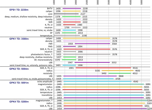
Overview of logs available for EPS1. BHTV, borehole televiewer; SGR, standard gamma ray; FMI, fullbore formation micro imager; FMS, formation micro scanner (resistivity); T, temperature; echo amplitude, amplitude of reflected acoustic signal; vs, shear wave velocity; vtube, tubewave velocity; SP, spontaneous potential; UBI, ultrasonic borehole imager; vstonely, stonely wave velocity.
3 FIRST DATA ASSESSMENT
Because of their various physical and chemical properties, clay minerals can be identified from geophysical borehole logs (after Ellis and Singer 2007).
Resistivity logs are sensitive to the structurally bound water inside the clay layers or on the surface of clay minerals.
The neutron porosity log is sensitive to hydrogen contained in water molecules.
Gamma ray logs identify abundances of radioactive isotopes included in the structure of clay minerals. Illite for example has a high K-content, montmorillonite integrates Th.
As the occurrence of clay minerals is strongly correlated with the vein alteration, one would expect higher clay content and consequently higher SGR values with increasing alteration grades. Vein alteration occurs mainly on big fractures or on zones with a high fracture density. In order to further investigate this correlation, a fracture density log for EPS1 is computed. This is achieved by counting the fracture density along the well in a sliding window of 1 m length and a sampling rate of 0.1 m. The limitation for fractures larger than the sampling rate is overcome by counting them also in the neighbouring interval. For calibration purposes, EPS1 is especially suited as data can be directly be derived from the core. The fracture fillings have been determined and a SCCL for the density of clay filled fractures was computed for EPS1. Henceforth, this log will be referred to as iSCCL. Following, the granite is subdivided into five groups of different alteration grades in order to investigate the relationship between alteration (i.e. clay content) and SGR values (Table 1).
Classification of the different lithologies into five qualitative alteration grades visually described from cutting analysis (Genter & Tenzer 1995).
| Alteration grade | Description of lithology, litholog (cuttings) |
|---|---|
| 0 – Fresh granite | Porphyritic granite, biotite-rich granite, K-feldspar megacrysts, kalifeldspar-rich granite, xenolith, |
| K-feldspar cumulate, microgranite, two-mica granite, hematized granite, leucogranite and propylitized granite | |
| 1 – Low alteration | Poorly hydrothermalized granite and altered porphyritic granite |
| 2 – Moderate alteration | Moderately altered granite and cataclased granite |
| 3 – Highly altered | Highly altered granite, breccia and crushed microbreccia |
| 4 – Extremely altered | Extremely altered granite, quartz vein, protomylonite, mylonitized granite and fracture zones |
Previous assumptions regarding higher SGR values with increasing clay content and higher alteration grade cannot be verified easily (Fig. 3). The computed iSCCL is plotted versus the SGR data of EPS1 and the alteration grade is illustrated colour-coded. The effect is probably caused by various primary minerals in the granitic matrix like biotite or K-feldspar, which can also incorporate radioactive isotopes. This makes it necessary to use the whole gamma spectrum of K, Th and U logs and to find a method to resolve the complex interaction of granitic matrix and clay minerals from these multidimensional logging data.
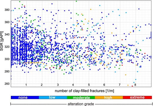
Crossplot of the clay-filled fracture density counted from the EPS1 core vs. SGR. The colour of the dots represents the alteration grade of the host rock. There is no correlation visible between the clay content, alteration grade and the SGR counts. The vertical lines occurring between 0 and 1 fracture per meter are artefacts of the 0.1 m precision of the clay-filled fracture density calculation.
4 BACKGROUND AND METHODOLOGY
The NNA is a method, which has proven itself in the application on multidimensional data in many fields. It is for example a common method in face recognition (e.g. Lawrence et al.1997) or in image processing (e.g. Cochocki & Unbehauen 1993), but it has also been used for geological tasks. In geological context, it has among others been applied for earthquake prediction (Alves 2006). Alves used a tool originally developed for financial analysis and applied it on the seismicity occurrence of the Azores. With this method, he successfully predicted the 1998 July and the 2004 July earthquakes. Singh (2005) applies an NNA on conventional logs like gamma ray, neutron and density logs for the porosity/permeability prediction of the Uinta Basin. Maiti et al. (2007), Chawathe (1994), Nikravesh (1998), Benaouda et al. (1999), Baldwin et al. (1990) and Rolon et al. (2009) use the NNA technique for facies prediction in different geological settings. Their works have in common that the NNA technique is used for the creation of synthetic logs for wells, where measurements are missing. More specifically, Rolon et al. (2009), Ayala Marín & García-Yela (2010), Dingding et al. (2006) train the network on wells, for which all desired logs are available and create synthetic logs by applying it on wells, where the data is incomplete. The obtained logs can replace real loggings, which cannot be measured as a consequence of low budgeting or technical reasons. An overview over the applications of NNA in the petroleum industry is given by Ali (1994). To our knowledge this study is the first application to use NNA for the detection of clay zones and the estimation of the amount of clay minerals in altered igneous rock for geothermal purposes.
Because of its flexibility and versatileness, the application of a neural network is suited to meet the challenge of identifying complex correlations between wall rock and measurements in multidimensional geophysical logging data. In this section the different aspects, which make the neural network suitable for the problem of identifying clayey fracture zones, are explained.
For this study the Schlumberger Software Techlog64 (version 2011.2.1) is used. The Techlog software package allows handling and interpreting a multitude of multiwell data. In addition to common statistical methods the software provides the possibility to evaluate logging data with more complex approaches like the NNA called ‘IPSOM’.
Basically, a neural network consists of an input and an output layer of numerous units called neurons. Each neuron is able to receive process and transmit information. While connected, input-units receive signals from the environment and output-units pass information to the environment. The kind of connection between these units is manipulated by weights, which control the transmission of information. The weights can be positive and negative and they can be of various magnitudes. Thus, the input of a neuron depends on the output or activity of the connected neurons and on the weight between them.
For our study, the Kohonen-algorithm (Kohonen 1984) is used. This algorithm works with a self-organizing map (SOM), which is a 2-D representation of the multidimensional network. It helps understanding, how data is organized and it allows basic manipulations of the computed network. The computing of the SOM consists of a training phase, where the network analyses the given input, and a propagation phase, where the acquired knowledge is tested. In the training phase, the input logs are classified, that is, each neuron is assigned different patterns of log response (Fig. 4a). Initially, the weights between the neurons are arbitrarily chosen. Then, the network selects an input vector and the activity of the output-neurons is calculated. The unit, which is most excited, is the one with the closest properties and the minimum distance to the input pattern. Then, the weights to this unit are adjusted in a way that the input vector is better approximated (Fig. 4b). The same, but in a weaker form, happens to the neighbouring units. The learning parameter, which determines, how much the weights are changed, is reduced after each cycle, so that the changes to the weights become smaller and smaller. This process is repeated until the predefined number of iterations is reached. If the number of cycles is large, the changes become continuously smaller and the network approaches a stable state.
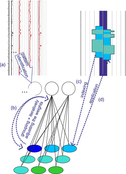
The neural network analysis with a Kohonen map from the input log (a) to the synthetic log (d). In detail: (a) Input logs give their information to the input neurons (empty circles) and the input data is classified in a map according to close patterns. (b) The weights between input and output neurons (coloured circles) are adjusted and the network unravels. The nodes can be illustrated on a 2-D SOM. (c) The indexing data set controls the clustering of the nodes. Each node is assigned to a certain group (illustrated by the different colours). (d) The network identifies similar patterns in the application data set and assigns them to the groups given by the index.
First, the network learns how the petrophysical properties and the reference classification (index) are correlated; this is the so-called supervised mode. In order to create synthetic logs representing the groups of the index-log, the nodes of the SOM have to be assigned to the respective index groups. This process is called the indexation of the map and it is done with the minimal distance method. Each pattern identified in the log corresponds to a certain index group given by the reference log. Nodes with similar properties are assigned to the same group, if the distance between the properties of the node and the group is minimal. Thus, each node of the SOM is assigned to the index node with the closest properties. The result of this process can be directly seen on the 2-D map (Fig. 4c), where the different groups are represented by different colours.
In the following propagation phase, the knowledge of the network stored in the weights of the neurons is tested in order to check its quality. Herein, this is achieved by applying the network on the input data and comparing it with the index log, which was initially given as a basis for learning. With application of the trained network on itself, patterns in the logs are grouped into neurons assigned to the group of the respective index neuron (Fig. 4d). By comparing the resulting log of the propagation phase with the index log, wrongly assigned units can be corrected and the result of the created synthetic log can be improved.
Among the parameters which affect the performance of the Kohonen map, are the number of iterations, the radius and the algorithm of the neighbourhood function, the learning parameter, the size of the SOM and the dimension of the network. The number of neurons should be adapted to the data. It should be considerably smaller than the number of input samples in order to achieve a proper learning and indexation. The number of iterations should be high enough for the network to converge to a stable state during the learning process. Kohonen (2001) suggests that the number of iterations should be at least 500-fold the number of output units. These parameter-effects will be discussed in the following section.
5 METHODOLOGY FOR THE IDENTIFICATION OF CLAY-BEARING FRACTURE ZONES USING AN NNA
5.1 Training of the NNA on the reference logs of EPS1
In the learning phase, the network is trained on the gamma ray logging data and the core fracture density log. The NNA is tested with SOM sizes of 10×10, 15×15, 20×20 and 25×25 nodes. After Kohonen (2001) the iteration numbers should then be at least 50 000, 112 500, 200 000 and 312 500. In this study, 120 000, 1 000 000, 3 000 000, respectively 5 000 000 cycles are applied and their results are compared in order to find optimum settings. The result of the learning process is a map of nodes with each of them representing a spectral composition of SGR, K, Th, U and fracture density data. Following, the nodes are indexed according to the iSCCL log. This way, the neurons of the map are categorized into five clay content groups [corresponding to 0–20 per cent, 20–40 per cent, 40–60 per cent, 60–80 per cent and 80–100 per cent of the maximum iSCCL value and numbered from 1 (low density) to 5 (maximum density)]. In the following propagation phase, the result will be processed in order to improve the correlation between the index and the modelled log. The procedure will be explained in the next chapter.
5.2 Testing the quality of the network by its application on the input data
The processing of the NNA is necessary to reassign nodes to the proper facies, which have been wrongly indexed. This is done in the propagation phase, where the network is reapplied on the input data to compare the reference log with the synthetic log. Improvement of the results is done manually by working on the SOM, on a 2-D representation of the network, the spectra for the index groups and the model log. As an example, the procedure is explained for an NNA with 100 nodes (Fig. 5).
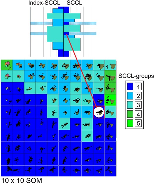
Self-organizing map: Each square of the map represents one node. Each node of the SOM reflects a specific spectral composition, which is displayed as a pie chart. The size of each portion is related to the intensity of the log response. The node colour represents the respective iSCCL group. Dots on the spectra of each square represent samples that define a node. The closer the dots are to the centre of the square, the closer their properties are to those of the index node. During processing the node responsible for the classification of a specific depth to one of the five clay content groups can be displayed. The corresponding node is marked with a white circle in the SOM and the depth interval is highlighted in light blue. By comparing for each group the probability to fit a node, poorly defined nodes can be redistributed to a different group.
Manual processing is necessary to avoid misinterpretations caused by influences of the rock matrix, but it has to be thoroughly decided, which combinations of log intensities show clay and which are caused by the granitic matrix. Different clay minerals, which have miscellaneous characteristics, excite different log responses that are mixed with the influence of the host rock. Therefore, the matrix lithology has always to be considered before reassigning a node.
6 RESULTS
The resulting SCCLs for different SOM sizes agree closely with the iSCCL (Fig. 6). The synthetic log for the map size of 25×25 nodes provides the best results. The synthetic clay log named SCCL 25×25 presented in Fig. 6 was created with a SOM of 625 nodes using 5 000 000 iterations for the network training.
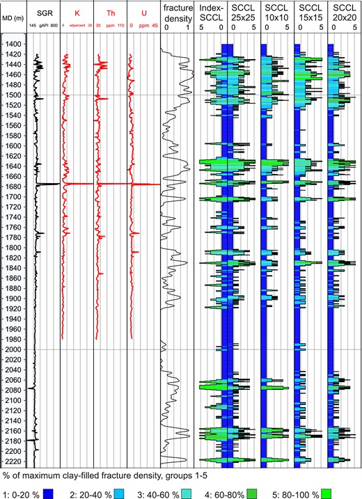
SCCLs for various SOM dimensions for EPS1 and the input logs SGR, K, Th, U, normalized core fracture density and the iSCCL. The fracture density and the iSCCL have been computed from core data and serves as a reference. The SCCL are the logs modelled using a SOM with different sizes. Accordance between iSCCL and SCCL: 10 × 10: 62.9 per cent, 15 × 15: 66.2 per cent, 20 × 20: 69.9 per cent, 25 × 25: 74.3 per cent.
To quantitatively analyse the quality of the modelled log, the percentage of correctly determined index groups is calculated. The model provides a great accordance with the index (Table 2). A major portion (74.3 per cent) of depth intervals has been correctly assigned and 90.7 per cent of the depth intervals deviates maximum 1 group from the index.
Percentage of depth intervals of the SCCL deviating by varying degrees from the iSCCL (rounded values). No deviation means that the SCCL matches the iSCCL, that is, the prediction of the SCCL is correct.
| Deviation from iSCCL | Depth intervals (per cent) |
|---|---|
| None | 74.3 |
| 1 group | 16.4 |
| 2 groups | 5.6 |
| 3 groups | 3.1 |
| 4 groups | 0.6 |
| Deviation from iSCCL | Depth intervals (per cent) |
|---|---|
| None | 74.3 |
| 1 group | 16.4 |
| 2 groups | 5.6 |
| 3 groups | 3.1 |
| 4 groups | 0.6 |
The network cannot only reconstruct the largest densities of clay-bearing fractures, but it is also able to assess their quantity (Fig. 6). The upper zone of high clay content and fracture density between 1400 and 1540 m is characterized by the formation of clay minerals from feldspars and a superposition of palaeoweathering. The medium part between 1540 and 1980 m penetrates porphyritic granite of different alteration and fracturation grades, while all gamma ray logs are available. The big fracture zone between 1620 and 1640 m, at 1660 m and at 1700 m depth are very well reconstructed in the SCCL. Even for the palaeo-alteration zone at the top of the granite to a depth of about 1550 m, where logs are sometimes very sensitive to the various alteration products, the model shows great accordance with the iSCCL.
The quality of the SCCL is not the same for the prediction of clay groups 1–5 (Fig. 7). The diagram shows for each iSCCL group the respective predicted group. The pie chart illustrates the sum of depth intervals covered by the respective groups. The prediction is most accurate for group 1 where the clay-filled fracture density is low (Fig. 7 left). If group 1 has been determined from core data, for 87 per cent of the respective depth intervals this group is really predicted by the SCCL. The prediction of group 2 is more uncertain and it is to 31.5 per cent misinterpreted as group 1. For the interpretation of the statistics it is also important to consider the decreasing number of depth intervals for higher density of clay-filled fractures.
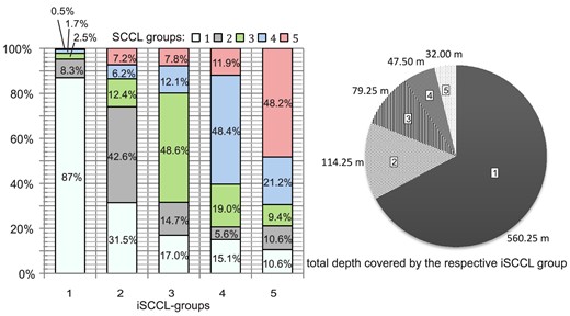
Left-hand panel: the graph shows for each iSCCL group belonging to a depth interval, which group is predicted by the model. The numbers inside the bars give percentage for each group rounded to one decimal. Right-hand panel: the figure shows for each group the total depth covered.
Even though the correct amount of clay is not in all cases properly determined, the deviations of the predicted model groups from the real ones are mostly only by one group, that is no more than 20 per cent more or fewer total clay content. So, the present model can distinguish between clay-filled fractures and fractures without clay. For the purpose of mapping potentially weak zones, this is a prerequisite.
7 DISCUSSION
7.1 Origin of deviations from the iSCCL
The largest clay-bearing fracture zones and the zones without clay can be reconstructed very well. Smaller zones are not fitted by the model. Examples for such zones are shown in Fig. 8. In some intervals, the model predicts more clay-filled fractures than there are (Fig. 8a). One reason for that is in the granitic rock matrix. The mentioned interval lies in a kalifeldspar cumulate (light-blue interval in the lithology log) with a naturally high K content. Therefore, the SGR and K readings of this zone are increased and the NNA interprets this as enrichment in clay minerals.
![Comparison of the clay model with other measured logs [lithology, neutron, short normal resistivity (SN), spontaneous potential (SP)]. The intervals (a), (b) and (c) marked with the red rectangle are zones, where the model predicts too much clay [rectangle (a)] or too little clay-[rectangles (b) and (c)]. In the lithology log, red intervals are standard granite, yellow is biotite-rich granite, light-blue is kalifeldspar cumulate, purple is xenolith, green is hydrothermalized granite.](https://oup.silverchair-cdn.com/oup/backfile/Content_public/Journal/gji/196/2/10.1093/gji/ggt423/2/m_ggt423fig8.jpeg?Expires=1716611322&Signature=1KW1C-2nUVd0cUo7T6HoPNrKGh4bXX6IR44XvGqq8ZK57LOZtyAgV5cXj7dARSZEg874lOaSc7GJTpiCM7-AmLt0~FYFZ1QfOz8GbgzzTHx9xXU2AFv8LlA0HM9cKEWqw1TJGFx~iLw1Zf2FR-LWInGkxZQ1S2Cpujh5d53iPVbrNg8RlGcYBLZXY8LMoLVrE8WqZaZp~hKINn8RolQk-OKGYj2C~CGWR6Kvqr91Z~na6PRUFGVUjppKP2zrvVypTawknBis07M9lM9OJOv-I9zlfc1WRibHbLuz52lk4VvwIFtbyYsWWLCmOR6-lZiR7WyGW~nrRGn~3lhDNRgajg__&Key-Pair-Id=APKAIE5G5CRDK6RD3PGA)
Comparison of the clay model with other measured logs [lithology, neutron, short normal resistivity (SN), spontaneous potential (SP)]. The intervals (a), (b) and (c) marked with the red rectangle are zones, where the model predicts too much clay [rectangle (a)] or too little clay-[rectangles (b) and (c)]. In the lithology log, red intervals are standard granite, yellow is biotite-rich granite, light-blue is kalifeldspar cumulate, purple is xenolith, green is hydrothermalized granite.
In a few zones the predicted density of clay-filled fractures is lower than it is observed in the core (Fig. 8b). The respective interval is in xenolithe, which possibly gives a different background signal than the standard granite and thus leads to an overestimation of the clay-fracture density. However, in some zones, where we observe such behaviour (e.g. Fig. 8c), the input data are incomplete. If one or more of the gamma ray logs is missing, the indexation is difficult and the prediction of the model has to be carefully assessed.
7.2 The sensitivity of the NNA configurations
Depending on the NNA configurations, the result of the model may change. In order to test the influence of the different parameters, the network was run several times using different numbers of nodes and clay groups. The results are discussed below.
The models for SOM sizes of 10 × 10, 15 × 15, 20 × 20 and 25 × 25 maps are compared in order to investigate the effect of a higher number of nodes. The respective SCCLs are shown in Fig. 6. Sizes larger than 25 × 25 are physically not reasonable as the number of input samples is too small to guarantee a proper learning and indexing. Using a higher number of nodes improves the resolution of the data and it gives the possibility to better assign the log responses to different groups (Table 3). This way, small nuances between index groups and nodes can be better captured. Fig. 6 compares the logs modelled with different SOM sizes. The resolution and the quality of the logs increase with increasing number of nodes (larger map). This is also confirmed by the statistical evaluation of correctly determined depth intervals (Table 3).
Comparison of the percentage of correctly modelled clayey fracture density groups for different input parameters of the NNA. The learning phase span 5 000 000 iterations. Ex., Example.
| Parameters | Ex. 1 | Ex. 2 | Ex. 3 | Ex. 4 | Ex. 5 | Ex. 6 |
|---|---|---|---|---|---|---|
| Size of SOM | 10 by 10 | 15 by 15 | 20 by 20 | 25 by 25 | 25 by 25 | 25 by 25 |
| Number of clay groups | 5 | 5 | 5 | 3 | 5 | 10 |
| Correctly determined intervals | 62.9 per cent | 66.2 per cent | 69.9 per cent | 84.2 per cent | 74.3 per cent | 50.0 per cent |
| Nodes:samples | 1:33 | 1:15 | 1:8 | 1:5.3 | 1:5.3 | 1:5.3 |
For the present model, five clay content groups (0–20 per cent to 80–100 per cent of maximum clay-bearing fracture density) are used. Using more groups makes the processing of the model a lot more complicated and the model is worse than for the model with only five groups. Only 50 per cent of the depth intervals can be correctly modelled by using 10 clay content groups. One reason for that is that the number of samples which are the basis for the definition of an index group is much lower (down to three samples) and no more representative. Furthermore, the sampling rate of the logs sets a limitation to the depth intervals belonging to the same clay content group. They are often as small as 0.25 m. When comparing this to the sampling rate of 0.15 m for gamma ray logging, such groups cannot be resolved from these logs as they are characterized by only one sampling point. Therefore, it is not considered reasonable to refine the resolution by using more index groups. A smaller number of groups (Example 4 (Ex. 4), Table 3) can improve the correlation between index and model, but the resolution is worse and informative value gets lost.
The NNA was run with different numbers of iterations. Different orders of magnitude between 100 000 and 5 000 000 have been compared and the learning process of the map been observed. At the beginning of the learning phase there are large changes in the spectra defining the nodes of the SOM until a nearly stable state is reached. After a sufficiently high number of iteration cycles, we can only observe very small changes in the map. The large number of degrees of freedom for larger sized maps is reflected by the required number of iterations. For the 10 × 10 map, the stable state was reached after 500 000 cycles, for the 25 × 25 map we used 5 000 000 iterations. Although a higher number of cycles also involves a longer computing time, it is better to use a preferably high number of iterations. Otherwise, the neuronal network has not completely adjusted to the input data and the result is neither representative nor reproducible. For this study the computing time was only few minutes, so we could easily apply high numbers of iterations, but for larger data sets this could be an important factor to consider.
Compared to the minimum 312 500 iterations postulated by Kohonen (2001), a factor 10 higher number was used During the learning process we could observe that the stable state for a 25 × 25 map was not reached at all after 312 500 iterations From this it is obvious that the postulated minimum is really an absolute minimum to obtain reproducible results but it is better to use a preferably high number of cycles and to observe the learning process in order to find the optimum settings.
Because of its iterative learning character, the exact weight distribution of a neural network can never be exactly reproduced in a further run. However, the resulting models and statistics of different runs of the SOM are very stable. This is a big advantage in the usage of NNA, as there are many ways to reach the goal. This is not the case, if the number of iterations is chosen too small or if the number of nodes of the SOM is not adapted to the input data. However, once the parameters are thoroughly chosen and the network calibrated with a high number of cycles to reach the stable state, the result will be approximately the same for each NNA.
7.3 The benefit of further geophysical logs for interpreting SCCLs
In order to identify logs that are useful to assess the certainty of modelled clay-zones, log responses in real clay zones in EPS1 are investigated. It is found that there is no log, on which all clay zones can be identified. The peaks of resistivity logs, especially the short normal (SN) log, often coincide with large amounts of clay (Fig. 8). The neutron log in contrast is sensitive to hydrogen atoms, which can be incorporated into the structure of clay minerals, but appears also in water molecules of fluids. However, peaks in the neutron log can only be observed in very large fracture zones with large amounts of clay. Smaller zones are not seen, which is possibly due to their low hydrogen content. From this log, we can only assess where the fractured zones are and where clay is likely to appear. The spontaneous potential (SP) log is one of the best indicators for clayey zones. Its peaks coincide with high clay amounts and the log resolution is also very good (Fig. 8). Also on this log not all clay zones can be seen and unfortunately, we do not have neutron logs for the deepest wells. The effect of using these logs as an additional input for the NNA is following discussed.
As they were sensitive to some of the clay bearing fracture zones, the NNA is run again three times, each time adding the neutron log, the SP log and the shallow resistivity log, respectively, to the original input. The addition of the SP log could improve the correspondence between iSCCL and SCCL from 74.3 to 78.0 per cent, while the SN log improved it to 75.5 per cent. The neutron log in contrast could not improve the result. The correspondence was only 61.1 per cent. One reason for that may be that the neutron log is sensitive to fractures in general, not only to clay filled fractures. The SP and SN log however, are sensitive to the charged elements of clay minerals and are thus better indicators for clay-bearing zones. Unfortunately, these methods are not standard logging techniques anymore and might not be available for other wells, on which a NNA should be applied.
7.4 Application of the NNA to other wells and its implication for rock mechanics and hydraulics
By application of the trained network on GPK1–4, SCCLs are created for the remaining wells. Comparing the SCCL of GPK1 (Fig. 9) with data of large microseismic events (Charléty et al.2007) reveals the occurrence of large earthquakes in GPK3 between 4500 and 4600 m depth, where the clay content is predicted very low. We observe brittle instead of ductile behaviour, which might be fostered by clays, and apparently the flow paths are permeable in this clay-poor zone. Otherwise, a pressure sufficiently high to create large seismic events could not have built up.
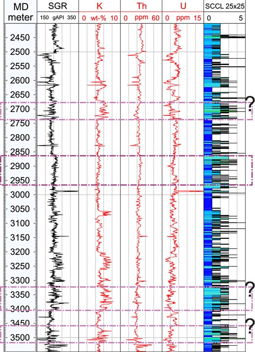
Section of the clay model for GPK1. Purple rectangle: aseismic zone after Cornet et al. (1997). Rectangles with question marks might be also aseismic because of their high clay content.
Cornet et al. (1997) found that near the bottom of GPK1 there is a zone, where aseismic movements took place on several fractures (Fig. 9) after hydraulic stimulation of the bottom hole section. GPK1 is cased down 2840 m depth. Below the casing shoe, some clay is predicted, where Cornet et al. identified aseismic zones. In order to further investigate the correlation between clay minerals in fractures, hydraulic properties and aseismic creep, more detailed studies need to be conducted. Such studies might also clarify, if the predicted high clay content zones (Fig. 8) are also potentially aseismic.
8 CONCLUSIONS AND OUTLOOK
A new methodology is presented, which can be used to predict the density of clay bearing fractures along boreholes with very good accuracy. The network has been trained on a data set consisting of SGR, K, Th and U and fracture density logs derived from image logs. The clay content data gathered from the EPS1 core served as a reference log (iSCCL). In order to obtain the best possible results the parameters of the NNA have been selected according to the input data. The best results could be obtained by choosing a SOM size of 25 × 25, which corresponds to a network with 625 nodes. A number of 5 000 000 learning cycles was found to be sufficient for the network to converge. The most significant limitations of the neural network have been found to be incomplete logging data or a complex interaction between rock matrix and clay minerals, which affects the gamma ray logs. In such intervals, which rarely occurred, clay bearing fractures are missed by the model or clay zones are spuriously predicted by the model. More than 90 per cent of the modelled intervals deviate maximum 20 per cent from the core derived reference log and 74 per cent of the intervals maintaining clay-filled fractures could be exactly reconstructed. Using additional logs like SP or resistivity could improve the results, but they might not always be available. Other logs like neutron could not improve the model, but they can be helpful for the interpretation of the SCCL.
So far, clay-bearing facies could only be reliably mapped in sedimentary environments. This neural network based technique makes it possible to locate clay-bearing zones also in crystalline environments, where the contrast in physical parameters is not sufficiently large to easily identify clay on well logs. The big advantage of this method is that it only needs standard geophysical loggings and can thus be widely applied. The resolution of the SCCLs depends on the resolution of the input logs only, so the synthetic logs can see small clay-bearing fracture zones down to the decimetre scale. Compared to the clay-localization using S waves/P waves or electrical logs (resistivity, conductivity, SP; Freund 1992; Titov et al.2010), the neural network based method allows a semi-quantitative estimate of the amount of clay present.
The SCCL of the non-cored well GPK1 showed clay-filled fractures in potential aseismic zones and low clay content in intervals, where large microseismic events occurred. The connection between the appearance of clay and the occurrence of seismicity and aseismic movements makes the NNA a powerful tool to identify potentially weak zones and hydraulic pathways. An application on the remaining Soultz wells GPK2–4 might therefore be used as an indicator for reservoir mechanics and hydraulic properties. The implication for clay-filled fractures on geomechanics and hydraulic rock properties will be proven in future studies.
The flexibility of neural networks makes this technique easily applicable to all kinds of environments and well logs. Therefore, it is not only interesting for geothermics but for all applications exploring and using the underground.
The authors are grateful to the EnBW for the financial support of the research, to the BRGM for providing the Soultz structural data and core pictures from EPS1, and to the GEIE EMC for providing the various geophysical data from the Soultz wells.
