


Abstract
Full waveform tomography (FWT) is a powerful velocity building method to exploit the full richness of seismic waveforms in complex media. Most applications today neglect the frequency-dependent amplitude decrease and phase velocity dispersion caused by intrinsic attenuation. In this study, we present a numerical investigation of the influence of attenuation on the recovered velocity model. Based on the generalized standard linear solid as rheological model, we incorporate attenuation into a 2-D time-domain acoustic FWT scheme. Attenuation is considered here as a modelling and not an inversion parameter. We investigate two reflection seismic experiments: (1) a visco-acoustic 1-D model and (2) a visco-acoustic version of the Marmousi model to which realistic quality factors are assigned. In the presence of soft rocks with pronounced absorption we observe a poor recovery of the velocity model when attenuation effects are not taken into account in the modelling. By considering an appropriate attenuation model in the forward modelling of the FWT, the accuracy of the reconstructed velocity model improves significantly in both cases. Even a homogeneous background quality factor model might allow a satisfactory recovery of the velocity model, provided that it is a quite good representation of the shallow structures. Our results suggest to consider attenuation as a smooth background modelling parameter in reflection seismic configurations to improve velocity model building by a purely acoustic inversion scheme.
1 INTRODUCTION
The aim of full waveform tomography (FWT) is to find a subsurface model which explains the recorded seismic data, that is, it iteratively minimizes the difference between observed and synthetic seismograms. In the majority of FWT applications, we face a multiparameter problem. In particular, attenuation might significantly affect amplitudes and phases of seismic signals due to frequency-dependent amplitude decrease and phase velocities (Causse et al.1999).
Nowadays, acoustic FWT is usually applied to recover the P-wave velocity model in transmission (e.g. Wang & Rao 2006; Maurer et al.2009) and reflection seismic configurations (e.g. Hu et al.2009; Bleibinhaus & Hilberg 2012). Most applications, thus neglect the impact of attenuation on seismic waveforms. The purpose of this work is to quantitatively investigate the validity of an acoustic FWT in the presence of attenuation.
There are two different ways to take attenuation into account. Attenuation may be used as a passive parameter, that is, as modelling parameter only. The aim is to improve the accuracy of the P-wave velocity model (e.g. Brenders & Pratt 2007). Alternatively, a multiparameter inversion, such as a visco-acoustic FWT (Liao & McMechan 1995, 1996; Askan et al.2007; Hak & Mulder 2008, 2011; Kamei & Pratt 2008) or the asymptotic visco-acoustic waveform inversion (Ribodetti et al.2004), involves attenuation as an additional inversion parameter.
Field data applications that take attenuation into account are mainly conducted in the frequency domain. Hicks & Pratt (2001) obtained reliable quality factor subsurface models from shallow seismic data recorded in the North Sea. Takam Takougang & Calvert (2011) reconstructed realistic velocity models from marine reflection data. They combined different inversion strategies, such as a multistage approach with incremental frequency selection (compare Bunks et al.1995; Sirgue & Pratt 2004) and separate inversion of near and far offsets. The vP-only inversion at low frequencies connected with the joint inversion for vP and QP at higher frequencies improved the recovery of both vP and QP models. Malinowski et al. (2011) applied a frequency-domain visco-acoustic FWT to wide-aperture seismic field data recorded in the Polish basin. They focus on the applicability of a visco-acoustic joint inversion for P-wave velocity vP and QP. They reconstructed satisfactory subsurface models for both vP and QP coinciding with the expected geology. In this context, Mulder & Hak (2009) discussed problems of a joint inversion with respect to short-aperture data in reflection seismics. They found that the ill-posedness of the inverse problem causes a very poor recovery of both phase velocity and attenuation. A brief overview of recent publications in this area is also given by Virieux & Operto (2009).
In this paper, we use a time-domain implementation to study the role of attenuation for weakly and strongly attenuative media in marine environments. We investigate the validity of an acoustic inversion scheme in presence of attenuation by systematically quantifying the errors in the inverted velocity model. Attenuation is incorporated as a passive parameter in forward modelling only. We apply a purely acoustic FWT including acoustic or visco-acoustic modelling to analyse and compare the impact of attenuation on the reconstruction of the velocity models from visco-acoustic reflection data sets.
Although this study concentrates on 2-D acoustic FWT in the time domain, it is also targeted to 3-D applications. While time-domain modelling (e.g. Bohlen 2002) is commonly used in 3-D applications, the high efficiency of 2-D frequency-domain modelling including a straightforward implementation of attenuation contrasts with highly demanding 3-D frequency-domain modelling using direct solvers (e.g. Wang & de Hoop 2011). However, there are robust and efficient frequency-domain approaches, such as iterative solvers (Plessix 2007). Furthermore, the time-domain approach has some advantageous features: straightforward time-windowing of data and the consideration of broad frequency bands (instead of single frequencies).
This work comprises implementation of finite-difference visco-acoustic modelling into the time-domain acoustic FWT and its application to visco-acoustic data. We choose two examples: a simple 1-D medium with a reflection acquisition geometry providing a high ray coverage and the 2-D Marmousi model with a towed streamer geometry. For both experiments we perform the same inversion tests. We investigate the resulting data misfits and model errors to demonstrate the footprint of attenuation on the recovered velocity models.
2 METHODOLOGY
The solution of the inverse problem is mainly based on the time-domain FWT introduced by Tarantola (1984) and Mora (1987). It comprises the adjoint method and the conjugate gradient method using the least-squares misfit definition. In contrast to the generalized derivations given by these authors, we assume some simplifications.
3 SYNTHETIC WAVEFORM TOMOGRAPHY EXPERIMENTS
We investigate the impact of attenuation in applications of acoustic FWT to visco-acoustic data with and without a passive QP model. Several acoustic full waveform inversion tests are employed to analyse the footprint of attenuation on vP inversion results. We analyse the effects of both visco-acoustic and acoustic modelling in acoustic FWT. The tests are applied to both a simple 1-D medium and the more complex Marmousi model using different initial vP and passive QP models. A list of all tests can be found in Table 1. To avoid unwanted side effects, some general restrictions and only necessary preconditioning features are applied. The FWT tests comprise the following set-up and constraints:
the P-wave velocity vP is the only inversion parameter,
apart from the gradient preconditioning mentioned above, we suppress the model update within the water layer due to the assumption of known model parameters,
Marmousi experiment: low-pass filtering of observed data and source wavelet over multiple stages is applied to improve the progress of the inversion (compare Bunks et al.1995; Sirgue & Pratt 2004),
stopping criterion for 1-D experiment to obtain most optimal results: FWT is unable to reduce data misfit (relative threshold value between two successive iterations is 0.0001 per cent), or it is not possible to compute a meaningful step length,
stopping criterion for shifting within multiple stages in the Marmousi experiment: due to high computational efforts, the relative threshold value of the data misfit between two successive iterations is 1 per cent.
List of all FWT tests for both the 1-D and the Marmousi experiment.
| FWT | Figures of vP results | Data | Modelling | Initial | Passive | |
|---|---|---|---|---|---|---|
| test | 1-D model | Marmousi | in FWT | vP model | QP model | |
| Reference | 6(a) | 10(a) | Acoustic | Acoustic | Smooth | – |
| Test 1 | 6(b) | 10(b) | Visco-acoustic | Acoustic | True | – |
| Test 2 | 6(c) | 10(c) | Visco-acoustic | Acoustic | Smooth | – |
| Test 3 | 6(d) | 10(d) | Visco-acoustic | Visco-acoustic | Smooth | True |
| Test 4 | 6(e) | 10(e) | Visco-acoustic | Visco-acoustic | Smooth | Smooth |
| Test 5 | 6(f) | 10(f) | Visco-acoustic | Visco-acoustic | Smooth | Homogeneous |
The reference computation applies acoustic inversion to acoustic data. It aims to show the performance of FWT for a given geology and geometry of both experiments. Tests 1 and 2 analyse the effect of attenuation on an acoustic inversion with acoustic modelling. Tests 3, 4 and 5 involve visco-acoustic modelling in acoustic FWT and investigate three different passive QP models in conjunction with the more realistic initial vP model (compare Table 1).
3.1 Synthetic experiment: layered 1-D model
The first experiment uses a 2-D model with a 1-D geology (hereinafter referred to as ‘1-D model’) consisting of four layers over a half-space: a water layer on top, followed by highly and weakly attenuative sedimentary rocks. The corresponding vP and QP models are shown in Fig. 1. Due to the occurrence of a thick layer with high attenuation on top of the sediments, this model represents a shallow marine environment. The total model size is 130 × 308 m with a spatial discretization of Δh = 0.5 m. However, due to the application of a PML (width = 15 m) in finite-difference modelling, all model-related figures are limited to the relevant area (excluding the PML layer). The acquisition geometry is located at the water surface and consists of 24 explosive sources with a spacing of 12 m as well as 278 hydrophones with a spacing of 1 m. For each shot gather all receivers are used. The resulting offsets range from 0.5 to 292.5 m. The source signal is a Ricker wavelet with a peak frequency fpeak = 80 Hz and the recording time of synthetic seismic data is 0.21 s.
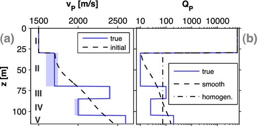
1-D experiment: Vertical cross-sections of the 1-D models: (a) True and initial velocity model. The range of phase velocity dispersion due to attenuation is illustrated by shaded areas. The layers are labelled with Roman numbers (water layer and half-space are denoted by ‘I’ and ‘V’, respectively). (b) shows true as well as smooth and homogeneous passive QP models (‘homogeneous’ with respect to the sub-seafloor area).
For visco-acoustic modelling, we determine the relaxation parameters such that we get an optimal representation of constant QP within the bandwidth of the seismic data (see Fig. 2b). Here, we define the bandwidth as the contiguous frequency range, wherein the decay of the amplitude spectrum with respect to the maximum amplitude is less than 10 dB (shaded areas in Fig. 2). The range of phase velocity dispersion of all layers is estimated within this bandwidth (see exemplary dispersion for the second layer with QP, 0 = 10 in Fig. 2c) and visualized by shaded areas in vertical sections across the 1-D medium (Fig. 1a). The aim is to analyse if the recovered vP model can be explained by the minimum and maximum velocity dispersion.
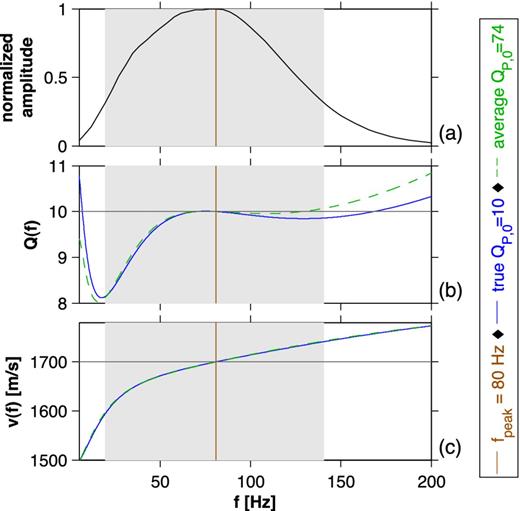
1-D experiment: Approximation of the quality factor. (a) shows the normalized amplitude spectrum of all observed visco-acoustic data. (b) and (c) illustrate the quality factor approximation and phase velocity dispersion for the second layer using the relaxation frequencies for QP, 0 = 10 and the average QP, 0 = 74. The shaded areas represent the bandwidth with respect to the observed data. The solid and dashed lines show Q(f) and corresponding phase velocity dispersion for the same relaxation frequencies fr, l = (1.202, 17.62, 179.4) Hz but true and average QP, respectively.
The approximation of relaxation parameters is based on the reference frequency f0 ≔ fpeak and an average QP, 0 = 74 computed from the true quality factor model within the sub-seafloor area (Fig. 1b). The acoustic velocity model vP, ref (Fig. 1a) is defined at f0, that is, no dispersion occurs at f0. The bandwidth of the seismic data is limited to |${\tilde{\Delta f} = \left[19.6, 141\right]\,{\rm Hz}}$|. This corresponds to a dynamic range of 2.8 octaves. Based on the rule of one relaxation mechanism per octave (Blanch et al.1995), we use three relaxation mechanisms. The resulting optimal set of relaxation frequencies is fr, l = (1.202, 17.62, 179.4) Hz. We found that it is not necessary to obtain relaxation frequencies for all quality factors of the true model, that is, it is not essential to provide models containing relaxation frequencies. Using the relaxation parameters computed from the average QP, 0 = 74, we obtain quite accurate approximations for all quality factors given in the 1-D model. An exemplary quality factor approximation is shown for the second layer with QP = 10 (Fig. 2b). Obviously, for this example the deviation in corresponding phase velocity dispersion is negligible (compare Fig. 2c).
The L1-based QP approximation error is given with respect to constant QP, 0 and is quantified within the seismic bandwidth. For all layers, we obtain acceptable approximation errors of about 3 per cent. While the approximation at reference frequency is perfect, the largest errors can be observed at the upper end of the bandwidth. These errors are nearly identical to those of the accurate QP approximation using exact QP values of each layer.
The smooth initial vP and passive smooth QP models for waveform tomography are generated by the application of a 2-D Gaussian filter (size 100 × 100 m, σ = 33) to the sub-seafloor area of the true model (see Figs 1a and b). In addition, Fig. 1(a) illustrates the minimum and maximum velocity dispersion with respect to the true vP and QP models.
A comparison of acoustic and visco-acoustic data computed from the true model at the central shot location is shown in Fig. 3. Due to very weak attenuation in water, the direct waves are nearly identical. At near offsets we can observe a quite good match in phases and amplitudes of the seafloor reflection. However, at larger offsets and for all later reflection events, there are significant differences between acoustic and visco-acoustic data. The phase misfit is explained by the highly dispersive properties of the second layer.
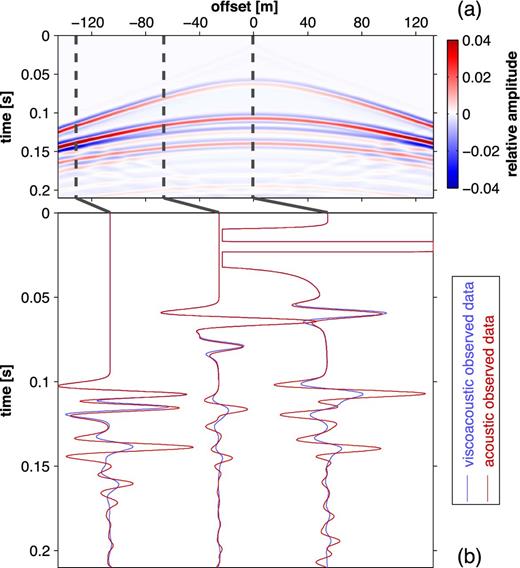
1-D experiment: (a) shows the difference between acoustic and visco-acoustic data for the central shot located at x = 160 m. It exhibits true amplitudes which are clipped to ±4 per cent of the maximum visco-acoustic amplitude. (b) illustrates traces at exemplary offsets. For a better visualization, they are normalized independently for each offset and the direct wave of the zero-offset trace is clipped. Acoustic and visco-acoustic amplitudes are still comparable.
In the following two paragraphs, we give a more detailed overview of the impact of attenuation on the seismic data by investigating both the sensitivity on model perturbations and the cycle-skipping phenomenon.
3.1.1 Sensitivity analysis
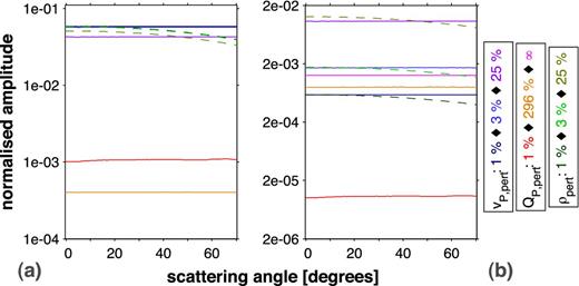
1-D experiment: Impact of scatterers in vP, QP or ρ on the partial differential wavefield (a) and the pure wavefield (b). (a) and (b) show the amplitude misfits (normalized to the amplitude of the unperturbed data) for different relative model perturbations as a function of the scattering angle and with respect to a homogeneous background medium. The normalized amplitude misfit for QP, perturb = ∞ in (a) amounts to 3.2 × 10⁻⁷.
The consideration of density in this work is a relevant simplification which might lead to insufficient model reconstructions in FWT applications influenced by media with inhomogeneous density. While vP modifies both phases and amplitudes, ρ only affects amplitudes of waveforms. The sensitivity of identical relative perturbations vP, perturb and ρperturb ranges within the same order of magnitude. In particular, at short apertures and thus small scattering angles, we can observe the maximum impact of ρperturb on the data (dashed graphs in Fig. 4b). From zero scattering angle to maximum scattering angle, the sensitivity ϵperturb(ρ) decreases by more than 30 per cent and thus describes a function of the scattering angle (according to Wu 1989).
3.1.2 Impact of attenuation on the cycle-skipping problem
Apart from the choice of the initial vP model, attenuation and, thus, dispersion might lead to cycle skipping. We compare both amplitude and phase misfits between visco-acoustic-observed data and the initial synthetic data of contrasting inversion tests 3 and 1 (see Table 1). On the one hand, the combination of the smooth initial vP model and the true QP model is used to analyse the impact of vP (see test 3). On the other hand, we choose the true vP model and neglect all information on attenuation to focus on the impact of QP (see test 1). Figs 5(a) and (b) (test 3) and Figs 5(c) and (d) (test 1) show the results of a time-frequency analysis applied to the data for the central source location. We applied a moving time window with a cosine shape and a length of one dominant cycle to the initial data, computed amplitude and phase spectra and calculated the average misfit (normalized to the observed data) with respect to the bandwidth.
The smooth initial vP model (Figs 1a and b) is a quite good representation of the shallow structures, that is, the seafloor reflection is characterized by a moderate amplitude misfit (Fig. 5a) and a non-existent phase misfit (Fig. 5b). All later events reveal stronger deviations in amplitudes and phase misfits up to half a cycle. However, phase-misfit discontinuities along the time direction might indicate the appearance of cycle skipping in test 3.
![1-D experiment: Time-frequency analysis of the residuals between observed data and the initial synthetic data for inversion test 3 (a and b) and test 1 (c and d). Both amplitude misfits (left column) and phase misfits (right column) are averages over the bandwidth of ${\tilde{\Delta f} = \left[19.6, 141\right]\,{\rm Hz}}$.](https://oup.silverchair-cdn.com/oup/backfile/Content_public/Journal/gji/195/2/10.1093/gji/ggt305/2/m_ggt305figa5.jpeg?Expires=1716403772&Signature=30WE2Yqw2BBLrAssR-R80ViW4xnOKLpZUXgZYa2c1Mqj5EVYMIT6uB-RuHDaiN8wVmi6XMr5OCngyYCodBYxAdGsR7KhocjGz-NzIs8IU2FQ93JLEVxemKAL1HIlNff3lClJWQiB-giaAvnvlHmB~uUDiId61Rc5m8QjPMmmt1Nxk0N9Z26pZQEN60iR3g2fGuaSI0c4UEaRY9gzT0eFGodj~pQu-7g5RLfGDw3C4a0xJDjQIFSca9ydYv9891Io2HhU7d0rjezv5mBxV~XcWGvO~n-HmD8N5PFywt8iGsTqq7EynNI4f8ApIpaSzTsv~iuQSeUhxXOc1aKTNUhEMg__&Key-Pair-Id=APKAIE5G5CRDK6RD3PGA)
1-D experiment: Time-frequency analysis of the residuals between observed data and the initial synthetic data for inversion test 3 (a and b) and test 1 (c and d). Both amplitude misfits (left column) and phase misfits (right column) are averages over the bandwidth of |${\tilde{\Delta f} = \left[19.6, 141\right]\,{\rm Hz}}$|.
In contrast, the choice of the true vP model as initial model and the assumption of an acoustic medium (e.g. compare infinite QP and QP = 10 in layer II) is reflected in significant amplitude misfits rather than phase misfits (Figs 5c and d). In particular, at the seafloor reflection, we can observe high amplitude misfits and the appearance of phase misfits, even though they are smaller than π/6. Altogether, the phase misfits increase up to half a cycle but do not show any discontinuous behaviour along the time direction. Consequently, we do not expect cycle skipping in test 1.
3.1.3 Inversion tests
Figs 6(a)–(f) show the results obtained by the reference FWT as well as from acoustic FWT of visco-acoustic data (compare Table 1), which will be discussed in the following. According to Fig. 1(a), all subfigures contain auxiliary plots of the dispersion range. The vertical section of all inversion results is computed by lateral averaging of a representative model area within the interval x = [80, 228] m. This avoids the involvement of unreliably recovered velocities, mainly related to the areas close to lateral model boundaries. Fig. 7 depicts the evolution of the corresponding data misfits and model errors.
A reliable interpretation of the effects caused by attenuation can be done by computing a reference result which comprises acoustic inversion of pure acoustic observed data. The nearly optimal conformity of the true and the final model (Fig. 6a) ensures the resolving power of FWT with respect to the given model and geometry. The reference FWT is characterized by the strongest reduction of both data and model error (see Fig. 7). It stops after 1762 iterations. Due to the computation of too small step lengths and the limited accuracy of single precision, the model update stagnated.
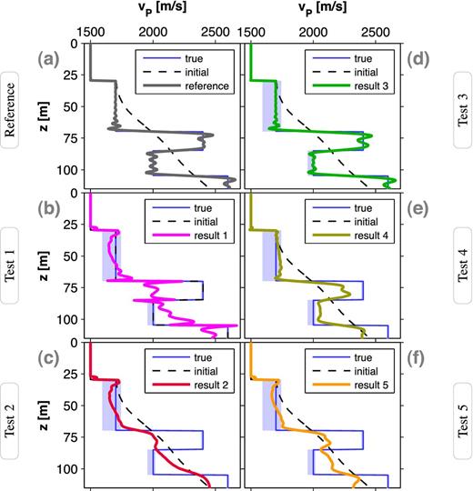
1-D experiment: (a) shows the FWT result for the acoustic reference computation. (b) to (f) illustrate the results of acoustic FWT applied to visco-acoustic data (tests 1–5). The shaded areas denote phase velocity dispersion.
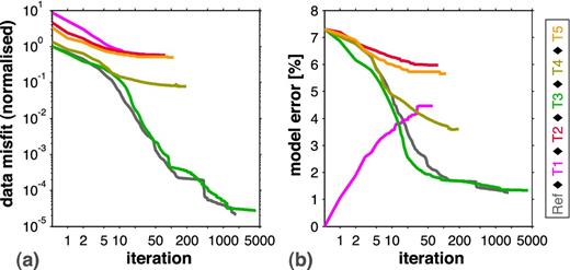
1-D experiment: (a) shows the evolution of the L2-based data misfit with respect to the number of iteration. The data misfit of the reference FWT (‘R’) is normalized to its own initial value. The data misfits of tests 1–5 (‘T1’–‘T5’) are normalized to the initial value of test 3 due to its best comparability with the reference FWT. (b) illustrates the evolution of corresponding L1-based model errors with respect to the true vP model. Colour coding is equivalent to Fig. 6.
Test 1 investigates the effect of neglecting QP information in an acoustic FWT applied to visco-acoustic data (Fig. 6b). In spite of using the true vP model as initial model, the FWT starts at the highest initial data misfit (Fig. 7a), which is reduced at the expense of the accuracy of the velocity model. On the one hand, the interface locations are still recognizable, but on the other hand, both a significant model error (increasing from 0 to 4.5 per cent, see Fig. 7b) and an artificial alteration of the velocity model can be observed. In particular, layer III is smeared heavily. Only layer II is recovered within the maximum range of velocity dispersion. This indicates that the effects of attenuation might be negligible in near-surface areas of the given model. Although we did not expect the occurrence of cycle skipping in this test (Figs 5c and d), the choice of a misfit definition being sensitive to amplitudes and thus the wrong explanation of amplitudes results in a failure of the inversion. The FWT of test 1 stops after 61 iterations due to the inability of computing a meaningful step length.
Test 2 represents a common FWT application (Fig. 6c). In this case we neglect QP and use the smooth initial vP model (Fig. 1a). The final velocity model is artificially recovered by the attempt of the FWT to explain the observed data. While the final vP model shows some improvements, it is still very similar to the initial model. Both the data and the model error are reduced slightly producing a smooth velocity model. Furthermore, the large-scale structures are comparable to the result of test 1. The FWT of test 2 stops after 77 iterations due to the inability of computing a meaningful step length. Although this inversion test already produced an unsatisfactory result, it still represents an ideal case with respect to the consideration of noise-free data. The appearance of noise might hide the effects of attenuation, particularly at later (multiple) reflection events. The misinterpretation of noisy data in terms of acoustic propagation effects leads to a further degradation of the vP model. Nevertheless, the primary reflections are crucial in reconstructing the large-scale structures of the 1-D model.
Test 3 includes the true QP model (Fig. 1b) as a passive model parameter. It can be clearly seen that the result resembles the acoustic reference result (Fig. 6d). The velocity of layer II is explained within the range of relevant phase velocity dispersion (see Fig. 2c). Especially in case of low attenuation (layer III and half-space), we do not observe this effect. Although the initial residuals indicated the appearance of cycle skipping (Figs 5a and b), the usage of the true QP model allows the correct explanation of amplitude misfits (in contrast to test 1). Thus, test 3 is characterized by a strong reduction of both data misfit and model error (see green plots in Figs 7a and b). This verifies the methodology of combining visco-acoustic modelling with the acoustic inversion scheme, that is, the gradient computation (6) and model update (9) use the relaxed model parameter but are based on the acoustic equations without any modification. The revocation of relaxation (12) yields an inversion result comparable to the reference result. The FWT of test 3 stops after 4191 iterations due to the threshold stop criterion mentioned above.
Test 4 shows a more realistic FWT application (Fig. 6e). We use the smooth passive QP model (Fig. 1b). The upper model areas are recovered quite well. In contrast to the previous result, we can observe a decreasing resolution of the velocity model with increasing depth. Although the passive QP model is a quite good approximation of the true model, a possible reason is the wrong fit of waveform amplitudes, that is, QP is overestimated in layers II and IV, while QP is underestimated in layers III and V resulting in a loss of high-frequency information. However, there is a remarkable reduction of both data and model error (see Fig. 7) resulting in a qualitatively good identification of layers and interfaces. The FWT of test 4 stops after 195 iterations due to the inability of computing a meaningful step length.
Test 5 deals with the simplest case of implementing attenuation (Fig. 6f). Here, we use a homogeneous passive QP model, that is, this model consists of the water layer over a homogeneous half-space with the average quality factor QP = 74. This test yields the smallest misfit reduction among all tests with visco-acoustic modelling (Fig. 7a) and a poor recovery of the velocity model which still is characterized by a high similarity to the initial model (compare Fig. 7b). The FWT of test 5 stops after 111 iterations due to the inability of computing a meaningful step length.
The observations for all tests coincide with the evolution of both the data misfit and the model error with respect to FWT iterations (Fig. 7a). The neglection of attenuation in tests 1 and 2 result in inappropriate velocity models. Surprisingly, the usage of true vP as initial model in test 2 causes a higher initial data misfit. However, both FWT tests end at the same high misfit level failing in the attempt to explain visco-acoustic data with acoustic modelling. Furthermore, the homogeneous QP model in test 5 yields a misfit evolution being nearly identical to test 2. In spite of incorporating attenuation, the result is very similar to the velocity model obtained in test 2. Obviously, in case of the 1-D experiment, the application of a homogenous passive QP = 74—which is an incorrect representation of the subsurface—is insufficient for a successful vP reconstruction. In contrast, the usage of the true QP model in test 3 results in a continuous reduction of the data misfit. This indicates the most optimal convergence to the global minimum of the misfit function. An acceptable trade-off is achieved by using the smooth QP model in test 4. In practice, a good QP model is usually unknown. Empirical relations can be used to derive a QP model from the initial velocity model. However, in general, they do not account for all rock types and physical conditions occurring in the given subsurface.
As mentioned above, a certain choice of a homogeneous passive QP model might cause unsatisfactory results. In addition, we performed an inversion using a homogeneous passive model with QP = 10 (representing layer II in Fig. 1b). In contrast to test 5, the inverted vP model shows a much better recovery of the upper layers. The reconstruction of layer II is nearly identical to the reference result. Layers III and IV show a small vP overestimation and underestimation, respectively. The average deviation from the true model is less than 3 per cent. However, the velocity of layer V is characterized by a large overestimation of about 13 per cent. Consequently, the passive QP model should rather be a good representation of the shallow structures of the model.
3.2 Synthetic experiment: Marmousi model
Using a modified section of the Marmousi-II model (Martin et al.2006, shown in Fig. 8), we repeat all previous investigations. The total model size is 3 × 10 km with a spatial discretization of Δh = 5 m. To reduce computational efforts velocities are clipped to vP = [1.5, 4] km s−1 (Fig. 8), which affects the deep salt layer extended from x ≈ 6 km to x = 10 km. The acquisition geometry consists of 32 explosive sources and a maximum number of 300 hydrophones per source. It forms a marine streamer geometry at the water surface moving from the right to the left model boundary. We choose a streamer length of 5980 m, a receiver spacing of 20 m and a nearest offset of 45 m. However, due to the existence of the right model boundary, only the receiver arrays for shots 20–32 provide the full streamer length, while shot one is equipped with the shortest streamer containing 18 receivers only. The source time function is a Ricker wavelet with a peak source frequency fpeak = 9 Hz. The recording time of seismic data is 5.15 s.
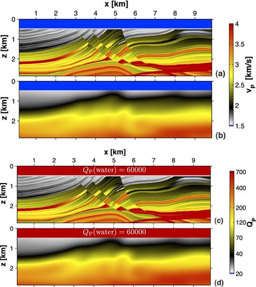
Marmousi experiment: (a) shows the true vP model and (b) depicts the initial vP model. (c) and (d) illustrate the true QP model and the smooth passive QP model.
The approximation of relaxation parameters is based on the reference frequency f0 ≔ fpeak, L = 3 and an average QP, 0 = 62 (harmonic mean) within the area beneath the seafloor. The bandwidth of the seismic data is limited to |${\tilde{\Delta f} = \left[3.3, 16.5\right]\,{\rm Hz}}$|. This corresponds to a dynamic range of 2.3 octaves. Consequently, we use a sufficiently high number of three relaxation mechanisms. The resulting optimal set of relaxation frequencies is fr, l = (0.1513, 1.925, 18.94) Hz. Based on the true model, both acoustic and visco-acoustic data as well as their residuals are shown for shot 24 located at x = 2555 m (Fig. 9). For a better illustration, the residual seismogram is clipped to ±4 per cent of maximum residual amplitude (Fig. 9a) and data traces are normalized to the maximum amplitude of visco-acoustic-observed data (Fig. 9b). Both amplitudes and phases of the waveforms are significantly affected by attenuation. While the strongest amplitude misfit is observed for the seafloor reflection, reflections from shallow structures and the refracted waves, the phase misfit continually increases with traveltime.
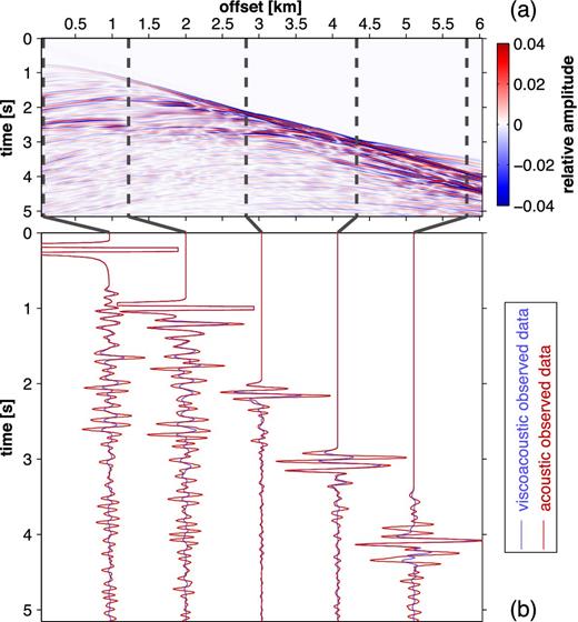
Marmousi experiment: (a) shows the residual seismogram with true amplitudes, which are clipped to ±4 per cent of the maximum visco-acoustic amplitude. The residuals are computed from acoustic and visco-acoustic data recorded at shot location x = 2555 m. (b) illustrates corresponding observed traces at exemplary offsets. For a better visualization they are normalized independently for each offset. Acoustic and visco-acoustic amplitudes are still comparable.
For the Marmousi model, we perform the same inversion tests as for the 1-D experiment (Table 1). The smooth initial vP model is generated by application of a 2-D Gaussian filter (size 1250 × 1250 m, σ = 51) to the sub-seafloor area of the true model vP, true (see Fig. 8b). While we use relation (15) to compute the smooth QP model (see Fig. 8d) from the initial smoothed vP model, the homogeneous passive QP model consists of the water layer over a half-space with the average quality factor QP = 62. All inversion tests are decomposed into multiple stages to reduce non-linearity of the inverse problem and to mitigate the cycle-skipping phenomenon: By application of low-pass filters, the inversion is performed for five frequency ranges, moving from low to high frequencies. The peak frequencies of low-pass-filtered data are not equidistantly spaced, as suggested by Sirgue & Pratt (2004): |${f_\mathrm{peak}=\left(1.7,\;2.6,\;3.7,\;5.0,\;9.0\right)\,{\rm Hz}}$|.
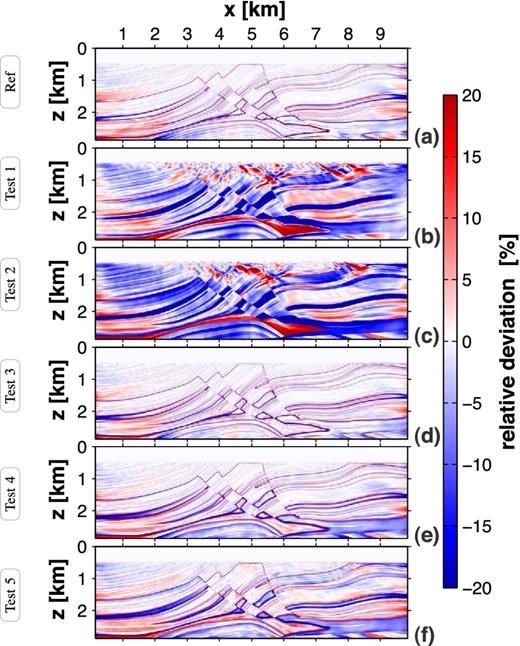
The inverted velocity models are shown in Fig. 10 and the corresponding relative deviations from the true model can be found in Fig. 11. For a better visualization, the deviation images are clipped to ±20 per cent. The actual maximum range is up to ±50 per cent. Due to the resolution limit of FWT of about half the wavelength, this is caused by the lack of very high frequencies. However, the incorporation of higher frequency contents and thus smaller wavelengths results in a finer finite-difference discretization (based on the grid dispersion criterion of approximately 16 grid points per minimum wavelength for a second-order finite-difference scheme). Consequently, in order to handle a reasonable grid size, very small-scale structures and high-contrast interfaces can not be recovered. Furthermore, Table 2 summarizes the data and model errors computed by eqs (13). For all FWT tests, it compares the change between initial and final errors.
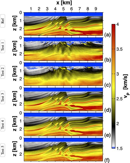
Marmousi experiment: (a)–(f) show the recovered vP models for acoustic reference FWT of pure acoustic data (a) and acoustic FWT of visco-acoustic data for tests 1–5 (b)–(f).
Marmousi experiment: List of errors ϵ with respect to the initial model vP|init and its corresponding initial data |$\mathbf {p}_\mathrm{init}$| as well as for the resulting model vP|result and corresponding data |$\mathbf {p}_\mathrm{result}$|. Using eqs (13), the errors are computed with respect to the true model vP|true and observed data |$\mathbf {p}_\mathrm{obs}$|. The arrows indicate the strength of error ratios |${\epsilon \!\left(\mathbf {p}_\mathrm{result}\right)/\epsilon \!\left(\mathbf {p}_\mathrm{init}\right)}$| and ϵ(vP|result)/ϵ(vP|init).
| Data error with respect to | Model error with respect to | Change of | ||||
|---|---|---|---|---|---|---|
| FWT | observed data (in per cent) | true model (in per cent) | Data | Model | ||
| |$\epsilon \!\left(\mathbf {p}_\mathrm{init}\right)$| | |$\epsilon \!\left(\mathbf {p}_\mathrm{result}\right)$| | ϵ(vP|init) | ϵ(vP|result) | error | error | |
| Reference | 53.4 | 0.0659 | 8.6 | 2.9 |  |  |
| Test 1 | 28.8 | 14.2 | 0.0 | 7.4 |  |  |
| Test 2 | 45.2 | 16.1 | 8.6 | 8.4 |  |  |
| Test 3 | 12.4 | 0.0204 | 8.6 | 3.1 |  |  |
| Test 4 | 13.2 | 0.186 | 8.6 | 4.1 |  |  |
| Test 5 | 19.2 | 2.69 | 8.6 | 5.0 |  |  |
| Data error with respect to | Model error with respect to | Change of | ||||
|---|---|---|---|---|---|---|
| FWT | observed data (in per cent) | true model (in per cent) | Data | Model | ||
| |$\epsilon \!\left(\mathbf {p}_\mathrm{init}\right)$| | |$\epsilon \!\left(\mathbf {p}_\mathrm{result}\right)$| | ϵ(vP|init) | ϵ(vP|result) | error | error | |
| Reference | 53.4 | 0.0659 | 8.6 | 2.9 | | |
| Test 1 | 28.8 | 14.2 | 0.0 | 7.4 | | |
| Test 2 | 45.2 | 16.1 | 8.6 | 8.4 | | |
| Test 3 | 12.4 | 0.0204 | 8.6 | 3.1 | | |
| Test 4 | 13.2 | 0.186 | 8.6 | 4.1 | | |
| Test 5 | 19.2 | 2.69 | 8.6 | 5.0 | | |
Marmousi experiment: List of errors ϵ with respect to the initial model vP|init and its corresponding initial data |$\mathbf {p}_\mathrm{init}$| as well as for the resulting model vP|result and corresponding data |$\mathbf {p}_\mathrm{result}$|. Using eqs (13), the errors are computed with respect to the true model vP|true and observed data |$\mathbf {p}_\mathrm{obs}$|. The arrows indicate the strength of error ratios |${\epsilon \!\left(\mathbf {p}_\mathrm{result}\right)/\epsilon \!\left(\mathbf {p}_\mathrm{init}\right)}$| and ϵ(vP|result)/ϵ(vP|init).
| Data error with respect to | Model error with respect to | Change of | ||||
|---|---|---|---|---|---|---|
| FWT | observed data (in per cent) | true model (in per cent) | Data | Model | ||
| |$\epsilon \!\left(\mathbf {p}_\mathrm{init}\right)$| | |$\epsilon \!\left(\mathbf {p}_\mathrm{result}\right)$| | ϵ(vP|init) | ϵ(vP|result) | error | error | |
| Reference | 53.4 | 0.0659 | 8.6 | 2.9 | | |
| Test 1 | 28.8 | 14.2 | 0.0 | 7.4 | | |
| Test 2 | 45.2 | 16.1 | 8.6 | 8.4 | | |
| Test 3 | 12.4 | 0.0204 | 8.6 | 3.1 | | |
| Test 4 | 13.2 | 0.186 | 8.6 | 4.1 | | |
| Test 5 | 19.2 | 2.69 | 8.6 | 5.0 | | |
Again, as described for the 1-D experiment, an acoustic inversion of pure acoustic data is used as the reference result (Fig. 10a). Considering the quite low peak frequency of the data, we can observe a good match of the reconstructed model and the true model (compare relative model deviation in Fig. 11a). Both data and model errors are reduced significantly (see Table 2).
In case of neglecting QP information (tests 1 and 2), the FWT is unable to recover subsurface structures properly from visco-acoustic data (Figs 10b and c). The resolution decreases dramatically with increasing depth causing a poor final vP model with high model and data errors (compare initial and final errors for tests 1 and 2 in Table 2, as well as Figs 11b and c).
In the following, we discuss the inversion progress of test 2 in more detail. Fig. 12 depicts the intermediate inversion results at the end of every frequency-filtering stage. Test 2 shows a satisfactory reconstruction of large-scale structures during the inversion of the low-frequency content (see Figs 12a–c). By including higher frequencies, artefacts appear in the upper sedimentary structures, while there are no improvements in deeper regions. In contrast, we can observe a destruction of large-scale structures which have already been recovered (Figs 12e and f). The minimum model error is obtained within the fourth stage with a peak frequency |${f_\mathrm{peak}=5.0\,{\rm Hz}}$| (Fig. 12d). Throughout the remaining inversion progress, the model error is increasing continuously, while the data misfit is decreasing. For a further investigation of this phenomenon, we repeat test 2 without multistage approach. We invert for the full frequency content at once and obtain a similar final result. However, the FWT skips the computation of an accurate intermediate result and directly produces an artificial model. Only until the sixth iteration there is a marginal improvement of the model. Apparently, the inversion of low-frequency contents is less sensitive to attenuation. This observation coincides with inversion strategies in visco-acoustic frequency-domain FWT applied by several authors. For example, Malinowski et al. (2011) analyse the sensitivity on attenuation in theoretical considerations and numerical experiments. Takam Takougang & Calvert (2011) use a similar multistage approach in a field data application. At low frequencies they only invert for vP. Later on, a combined inversion for vP and QP is applied.
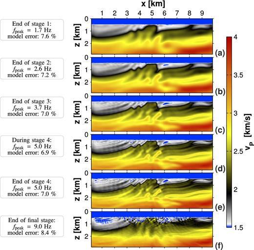
Marmousi experiment: (a)–(f) show the evolution of the vP model with respect to the inversion progress for the test 2. (a)–(c), (e) and (f) illustrate intermediate vP models at the end of each stage of low-pass filtering. (d) shows the model with the lowest model error (for comparison: the model error of the initial model is 8.6 per cent). (f) corresponds to Fig. 10(c).
Obviously, tests 1 and 2 demonstrate that the choice of the initial vP model does not affect significantly the outcome of the acoustic inversion of visco-acoustic data within the framework of the Marmousi experiment. In both cases, the velocity model is artificially altered in order to minimize the data misfit (compare increased model errors in Table 2). The misfit between visco-acoustic-observed data and acoustic synthetic data is mapped to the velocity model.
In contrast to tests 1 and 2, the involvement of a QP model improves the vP recovery significantly. Using QP, true as passive parameter, as performed in test 3, the reconstructed vP model is comparable to the optimal acoustic reference result (Figs 10d and 11d). Test 4 employs the smooth QP model and, thus, is the most realistic case. Considering this imperfect QP information, the FWT produces a satisfactory vP model (see final result in Fig. 10e and the model deviation in Fig. 11e). Although the smooth QP model does not allow the reconstruction of a vP model with high resolution, the comparison of test 4 with test 3 only shows a minor increase of the model error (Table 2). Even the implementation of a homogeneous QP information within the sub-seafloor region yields a surprisingly good result (Figs 10f and 11f). Apart from decreasing vP resolution with increasing depth, the qualitative Marmousi geology is clearly notable.
In general, the Marmousi experiment resembles the results of the 1-D experiment. In case of test 5, we observe different performances of the FWT. For both examples, there is a nearly identical reduction of the data misfit. However, in case of the Marmousi experiment, there is a significantly stronger reduction of the model error (42 per cent versus 25 per cent for the 1-D example). This observation is explained by the choice of the homogeneous QP model. For example, there is a huge QP discrepancy between the second layer of the true 1-D model and homogeneous model (true QP = 10 versus passive QP = 74). This causes incorrect data and an artificial model reconstruction. In contrast, there is a much better match of the homogeneous model and the upper structures of the Marmousi model (the arithmetic mean value of the true model and homogeneous QP = 62 are equivalent for depths 470 m ≤ z ≤ 1830 m). Concluding, a good QP model should be a good representation of the upper sub-seafloor regions.
4 CONCLUSIONS
In this work, we investigate the impact of attenuation on 2-D acoustic FWT in the time domain. The acoustic inversion scheme is applied to two visco-acoustic data sets generated for a 1-D structured model and the Marmousi model. The neglection of attenuation as a passive modelling parameter causes an unsuccessful recovery of the vP model. The attenuation-related data misfit is mapped to the velocity model by generating remarkable artefacts. If we use the true velocity model as an initial model, then the footprint of attenuation can be clearly observed in the artificially altered vP model. Although the impact of scattering QP structures on the data is a second-order effect, the influence of attenuation along the wave path in these reflection experiments is not negligible.
The application of a passive QP model significantly improves the vP model reconstruction. The usage of a smooth QP model results in a sufficient near-surface recovery of vP but the resolution is decreasing with increasing depth. This is caused by an attenuation-related loss of high-frequency information with increasing depth. Depending on the deviation from the true QP model, the choice of a homogeneous QP model increases the risk of an unsatisfactory vP recovery (see 1-D experiment).
In case of the appearance of soft sediments, the FWT has to take attenuation into consideration. The availability of a sufficiently good passive quality factor model allows the reconstruction of a reliable velocity model by applying the acoustic inversion scheme. However, such an appropriate good model does not necessarily have to be characterized by a high complexity being close to the true model. For example, the passive involvement of QP, which is derived from the initial vP model, might significantly improve the resolution of the vP model, provided that the QP model is at least an appropriate representation of the uppermost subsurface structures. In conclusion, it is not advisable to neglect attenuation or to use potentially poor attenuation information in FWT applications to real data recorded in marine environments with soft sediments.
This work was performed within the programme Geotechnologien funded by the German Ministry of Education and Research (BMBF) and the German Research Foundation (DFG)—grant 03G0752. It is also supported by the Verbundnetz Gas AG and the sponsors of the Wave Inversion Technology consortium (WIT). In particular, we want to thank the reviewer S. Operto and the editor J. Trampert for very helpful and constructive comments. The FWT computations were performed on the supercomputers JUROPA at Jülich Supercomputing Centre and HP XC3000 at the Karlsruhe Institute of Technology as well as on the bwGRiD cluster computers at several Baden-Württemberg state universities.
REFERENCES
APPENDIX: VISCO-ACOUSTIC MODELLING IN THE TIME DOMAIN
The implementation of attenuation into acoustic or elastic modelling has been described by numerous authors (e.g. Liu et al.1976; Emmerich & Korn 1987; Carcione et al.1988a,b; Robertsson et al.1994; Blanch et al.1995; Bohlen 2002). In modelling of frequency-domain FWT (e.g. Pratt 1999), the intrinsic attenuation is included quite easily by introducing complex velocities (Johnston 1981). In contrast, this direct implementation of attenuation is not possible in the time domain and must be approximated by a suitable rheology, which is represented by the generalized standard linear solid (GSLS) (Liu et al.1976). It consists of a parallel connection of a Hooke and L Maxwell bodies. The Hooke body represents pure acoustic properties. A Maxwell body consists of a Hooke and a Newton body where the latter one characterizes the viscosity of the medium. Thus, attenuation is described by L relaxation mechanisms.
Finally, the 2-D modelling comprises (10 + L) equations:
one equation for the update of pressure p,
two equations for the update of particle velocities wx and wy,
L equations for the update of memory variables rl,
seven equations for additional auxiliary PML variables ux, uy, θ, ϕx, ϕy, φ and ψ.
