Wave propagation across non-linear rock joints based on time-domain recursive method

Abstract

1 INTRODUCTION

In the previous paper (Li et al.2012), a time-domain recursive method (TDRM) was presented to study stress wave propagation across a set of parallel joints. Based on the stress wave interaction with a joint and the time-shifting function for wave propagation between two adjacent joints, the wave propagation equation in a differential form was derived. The TDRM was applied for the cases of normal and oblique incidence onto a single joint or a joint set with linearly elastic property. For wave propagation across joints with non-linear property, the analysis is much more complex and not readily available, especially for an oblique incidence.

The natural rock joints are generally non-welded, large in extent and small in thickness, and have relative deformation, such as opening, closure and slip under normal and shear stresses (Barton 1973; Brown & Scholz 1986; Daehnke & Rossmanith 1997; Zhao 1997; Pyrak-Nolte & Morris 2000). Many researches have shown that the deformational behaviour of a joint is generally non-linear (Goodman 1976; Bandis et al.1983; Zhao et al.2008; Li & Ma 2009) if the joint is filled with infilling materials and the magnitude of stress waves is sufficient to result in the non-linear normal displacement and relative slip of the joint. Among the joint models, the Barton–Bandis model (B–B model; Bandis et al.1983) has been widely used to describe the joint normal property. From the dynamic test results, a dynamic B–B model for the dynamic normal behaviour of rock joints was suggested (Zhao et al.2008). In addition, the shear strength of a smooth joint was usually described as functions of a normal effective stress and a frictional angle (Barton 1973; Zhao 1997). For nature rock joints, the peak frictional angle varies in the range of 35–45°.

Wave propagation across a single joint or multiple joints with non-linear behaviour has been studied by many researchers. For example, Miller (1977, 1978) analysed normal S-wave attenuation across a single joint with a slip-rate-dependent frictional model. Based on the experiments conducted by Pyrak-Nolte et al. (1990), Hildyard & Young (2002) and Hildyard (2007) numerically modelled wave propagation across multiple joints/fractures and introduced the stress dependency and the non-linear property of the hyperbolic joint stiffness relation (Bandis et al. 1983). Zhao et al. (2006b,c) adopted the method of characteristics (MC) for a normally incident longitudinal-(P-) or transverse-(S-)wave across a set of parallel joints. Based on the interaction between the stress wave and a rock joint, Li et al. (2011) analysed wave propagation across the joint with an arbitrary impinging angle. In their research, the B–B model and the slippery model were respectively used to represent the normal and shear properties of the joints.

The aim of this paper is to analyse wave propagation across a set of parallel joints with non-linear property using the TDRM and to better understand the effect of relevant parameters on wave attenuation in a rock mass. The incident P- or S-wave impinge on the joints obliquely. The wave propagation equation across non-linear rock joints is firstly established. Comparison between the transmitted waves for waves propagating across linear and non-linear joints is then conducted. The calculation results from TDRM are also compared with those from the existing methods for some specific cases, including a normal incidence across a set of parallel joints and an oblique incidence across a single joint. Parametric studies are finally carried out with respect to the incident angle, the joint spacing, the amplitude of an incident wave and the maximum allowable joint normal closure.

2 TDRM FOR WAVE PROPAGATION ACROSS JOINTED ROCK MASS

2.1 Problem description

A rock mass with a set of parallel joints is shown in Fig. 1(a), where the rocks between joints are identical, linear, isotropic and homogeneous. The Young's modulus and the density of the intact rock are denoted as E and ρ, respectively. Each joint is considered as a non-welded contact interface, which is planar, large in extent and small in thickness compared to the wavelength. Define S and N as the joint spacing and the joint number in the rock mass, respectively.

When a plane P- or S-wave impinges on the discontinuous rock mass, both reflection and transmission take place (Kolsky 1953; Johnson 1972). The propagation direction of the plane wave is taken to be in the x–z-plane and the interfaces of the joints are considered to be in the x–y-plane, as shown in Fig. 1(a). The symbols RR denotes right-running P or S wave, and LR denotes left-running P or S wave. In fact, there is a derivation in the ray path for wave propagation across the joints, as shown in Fig. 1(a). This is caused by the joint which is usually considered as a soft layer with one thickness, as shown in Fig. 1(b). If the effect of the joint thickness on wave propagation is not considered, the deviation in the ray path can be ignored. And no matter whether the joints are linear or non-linear elastic, the propagation of the plane waves should satisfy Snell's law according to the Fermat's principle of least time. Therefore, the emergence angles of the reflected and transmitted P waves are both equal to the angle of the incident P wave, so are the emergence angles of the incident, reflected and transmitted S waves. In other words, the angles of the reflected, transmitted and incident P or S waves are equal to each other. Define α and β as the emergence angles of the incident P and S waves, respectively, and α_c and β_c as the critical angles of the incident P and S waves, respectively. Here, we only study the case of 0 ≤ α < α_c and 0 ≤ α < α_c, where α_c and β_c are the critical angles and α_c = 90° and β_c = sin ^{− 1}(c_s/c_p) from Snell's law.

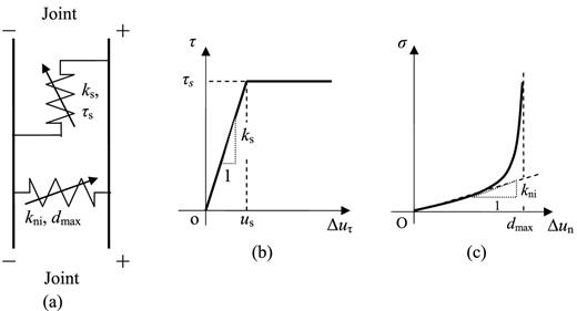
Assume that the joints have non-linear and slippery behaviour, for example, the B–B model for the normal behaviour and the Coulomb-slip model for the shear behaviour, as shown in Fig. 2, where k_ni is the initial normal stiffness and d_max is the maximum allowable normal closure of the joint, τ_s is the shear strength, u_s is the critical relative slip, k_s is the linear deformable slope and Δu_n and Δu_τ are the closure and the relative slip of the rock joint.

Figure 1.

Open in new tabDownload slide

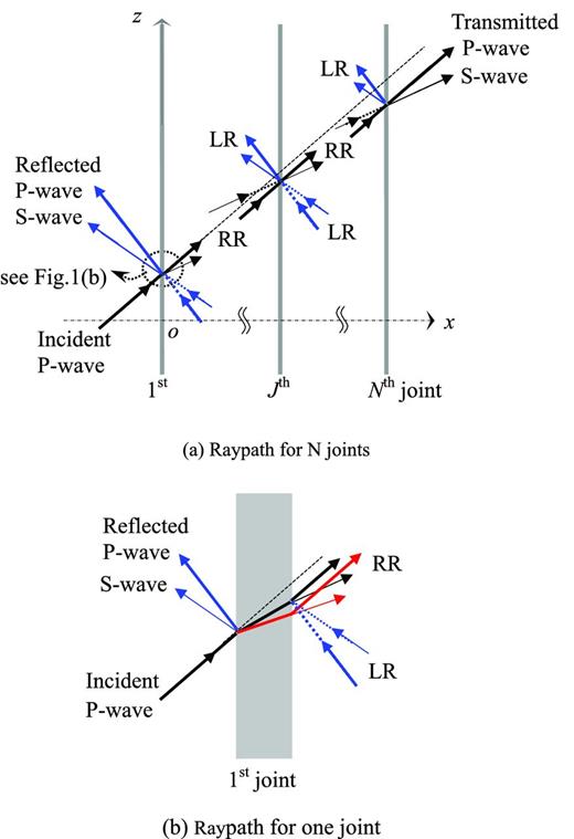
Schematic view for wave propagation across a set of parallel joints (LR represents left-running P or S wave, RR for right-running P or S wave).

Figure 2.

Open in new tabDownload slide

Rock joints with non-linear and slippery behaviour.

For the present problem, when the incident wave propagates across a set of joints and is reflected multiple times among the joints, there only exist four waves propagating in four directions, that is, the right-running (RR) P and S waves and the left-running (LR) P and S waves (Li et al.2011), as shown in Fig. 1.

The detailed derivation process can be found in the Appendix for the stresses and the velocities for the two sides of a joint, when the RR and LR P waves and the RR and LR S waves propagate across the joint.

2.2 Wave propagation across a joint

2.3 Wave propagation between two adjacent joints

2.4 Wave propagation equation

For a joint with non-linear and slippery behaviours, there are two possible shear deformation modes, that is, the elastic mode when |Δu_τ| < u_s and the relative slip mode when |Δu_τ| ≥ u_s. The following analysis is to derive the equations for wave propagation across joints with the two modes.

1. The elastic mode for |Δu_τ| < u_s. Substituting the stress expressions, that is, eqs (A10)–(A11) (see the Appendix) into eq. (1), and the velocity expressions, that is, eqs (A12)–(A13) into eq. (4), the wave propagation equation across a joint can be derived and expressed as a matrix form, that is

   \begin{equation} \left[ {\begin{array}{*{20}c} {v_{{\rm l}p}^ - } \\ {v_{{\rm l}s}^ - } \end{array}} \right]_{i,J} = - B^{ - 1} A\left[ {\begin{array}{*{20}c} {v_{{\rm r}p}^ - } \\ {v_{{\rm r}s}^ - } \end{array}} \right]_{i,J} + B^{ - 1} A\left[ {\begin{array}{*{20}c} {v_{{\rm r}p}^ + } \\ {v_{{\rm r}s}^ + } \end{array}} \right]_{i,J} + \left[ {\begin{array}{*{20}c} {v_{{\rm l}p}^ + } \\ {v_{{\rm l}s}^ + } \end{array}} \right]_{i,J} \end{equation}

   (8)

   \begin{equation} \left[ {\begin{array}{*{20}c} {v_{{\rm r}p}^ + } \\ {v_{{\rm r}s}^ + } \end{array}} \right]_{i + 1,J} = - C^{ - 1} D\left[ {\begin{array}{*{20}c} {v_{{\rm l}p}^ + } \\ {v_{{\rm l}s}^ + } \end{array}} \right]_{i + 1,J} + C^{ - 1} E\left[ {\begin{array}{*{20}c} {v_{{\rm r}p}^ + } \\ {v_{{\rm r}s}^ + } \end{array}} \right]_{i,J} + C^{ - 1} F\left[ {\begin{array}{*{20}c} {v_{{\rm l}p}^ + } \\ {v_{{\rm l}s}^ + } \end{array}} \right]_{i,J} + C^{ - 1} G\left[ {\begin{array}{*{20}c} {v_{{\rm r}p}^ - } \\ {v_{{\rm r}s}^ - } \end{array}} \right]_{i,J} + C^{ - 1} H\left[ {\begin{array}{*{20}c} {v_{{\rm l}p}^ - } \\ {v_{{\rm l}s}^ - } \end{array}} \right]_{i,J} \pm C^{ - 1} I\tau _{s0} , \end{equation}

   (9)

   where A to H are the matrix parameters, or

   \begin{equation} A = C = \left[ {\begin{array}{*{20}c} {z_p \cos 2\beta } & \quad {z_s \sin 2\beta } \\ {z_p \sin 2\beta \tan \beta /\tan \alpha } & \quad { - z_s \cos 2\beta } \end{array}} \right] \end{equation}

   (10)

   \begin{equation} B = D = \left[ {\begin{array}{*{20}c} {z_p \cos 2\beta } & \quad { - z_s \sin 2\beta } \\ { - z_p \sin 2\beta \tan \beta /\tan \alpha } & \quad { - z_s \cos 2\beta } \end{array}} \right] \end{equation}

   (11)

   \begin{equation} E = \left[ {\begin{array}{*{20}c} {z_p \cos 2\beta - \Delta t \cdot \overline {k_n } \cos \alpha } & \quad {z_s \sin 2\beta - \Delta t \cdot \overline {k_n } \sin \beta } \\ {z_p \sin 2\beta \tan \beta /\tan \alpha - \Delta t \cdot k_s \sin \alpha } & \quad { - z_s \cos 2\beta + \Delta t \cdot k_s \cos \beta } \end{array}} \right] \end{equation}

   (12)

   \begin{equation} F = \left[ {\begin{array}{*{20}c} {z_p \cos 2\beta + \Delta t \cdot \overline {k_n } \cos \alpha } & \quad { - z_s \sin 2\beta - \Delta t \cdot \overline {k_n } \sin \beta } \\ { - z_p \sin 2\beta \tan \beta /\tan \alpha - \Delta t \cdot k_s \sin \alpha } & \quad { - z_s \cos 2\beta - \Delta t \cdot k_s \cos \beta } \end{array}} \right] \end{equation}

   (13)

   \begin{equation} G = \left[ {\begin{array}{*{20}c} {\Delta t \cdot \overline {k_n } \cos \alpha } & \quad {\Delta t \cdot \overline {k_n } \sin \beta } \\ {\Delta t \cdot k_s \sin \alpha } & \quad { - \Delta t \cdot k_s \cos \beta } \end{array}} \right] \end{equation}

   (14)

   \begin{equation} H = \left[ {\begin{array}{*{20}c} { - \Delta t \cdot \overline {k_n } \cos \alpha } & \quad {\Delta t \cdot \overline {k_n } \sin \beta } \\ {\Delta t \cdot k_s \sin \alpha } & \quad {\Delta t \cdot k_s \cos \beta } \end{array}} \right] \end{equation}

   (15)

   \begin{equation} I = \left[ {\begin{array}{*{20}c} 0 \\ 0 \end{array}} \right]. \end{equation}

   (16)
2. The relative slip mode for |Δu_τ| ≥ u_s. Putting eqs (A10)–(A11) into eq. (1) and eqs (A12)–(A13) into eq. (5), the wave propagation equation is still in the form of eqs (8) and (9), while the matrixes A to H are

   \begin{equation} A = \left[ {\begin{array}{*{20}c} {z_p \cos 2\beta } & \quad {z_s \sin 2\beta } \\ {z_p \sin 2\beta \tan \beta /\tan \alpha } & \quad { - z_s \cos 2\beta } \end{array}} \right] \end{equation}

   (17)

   \begin{equation} B = \left[ {\begin{array}{*{20}c} {z_p \cos 2\beta } & \quad { - z_s \sin 2\beta } \\ { - z_p \sin 2\beta \tan \beta /\tan \alpha } & \quad { - z_s \cos 2\beta } \end{array}} \right] \end{equation}

   (18)

   \begin{equation} C = \left[ {\begin{array}{*{20}c} {z_p \cos 2\beta } & \quad {z_s \sin 2\beta } \\ {z_p \sin 2\beta \tan \beta /\tan \alpha \mp z_p \cos 2\beta \tan \varphi } & \quad { - z_s \cos 2\beta \mp z_s \sin 2\beta \tan \varphi } \end{array}} \right] \end{equation}

   (19)

   \begin{equation} D = \left[ {\begin{array}{*{20}c} {z_p \cos 2\beta } & \quad { - z_s \sin 2\beta } \\ { - z_p \sin 2\beta \tan \beta /\tan \alpha \mp z_p \cos 2\beta \tan \varphi } & \quad { - z_s \cos 2\beta \pm z_s \sin 2\beta \tan \varphi } \end{array}} \right] \end{equation}

   (20)

   \begin{equation} E = \left[ {\begin{array}{*{20}c} {z_p \cos 2\beta - \Delta t \cdot \overline {k_n } \cos \alpha } & \quad {z_s \sin 2\beta - \Delta t \cdot \overline {k_n } \sin \beta } \\ 0 & \quad 0 \end{array}} \right] \end{equation}

   (21)

   \begin{equation} F = \left[ {\begin{array}{*{20}c} {z_p \cos 2\beta + \Delta t \cdot \overline {k_n } \cos \alpha } & \quad { - z_s \sin 2\beta - \Delta t \cdot \overline {k_n } \sin \beta } \\ 0 & \quad 0 \end{array}} \right] \end{equation}

   (22)

   \begin{equation} G = \left[ {\begin{array}{*{20}c} {\Delta t \cdot \overline {k_n } \cos \alpha } & \quad {\Delta t \cdot \overline {k_n } \sin \beta } \\ 0 & \quad 0 \end{array}} \right] \end{equation}

   (23)

   \begin{equation} H = \left[ {\begin{array}{*{20}c} { - \Delta t \cdot \overline {k_n } \cos \alpha } & \quad {\Delta t \cdot \overline {k_n } \sin \beta } \\ 0 & \quad 0 \end{array}} \right] \end{equation}

   (24)

   \begin{equation} I = \left[ {\begin{array}{*{20}c} 0 \\ 1 \end{array}} \right]. \end{equation}

   (25)

Eqs (8), (9), (26) and (27) are the wave propagation equations for incident P or S wave across a set of parallel joints when the property of the joints is non-linear or satisfies the Coulomb-slip model. If | $ \overline {k_n }$| is equal to k_ni, the normal property of rock joints becomes linearly elastic and eqs (8), (9), (26) and (27) for the elastic mode, that is, |Δu_τ| < u_s can be simplified as the wave propagation equation derived by Li et al. (2012).

Among eqs (8), (9), (26) and (27), eqs (8) and (9) describe wave propagation across a joint and eqs (26) and (27) describe wave propagation between two adjacent joints.

The incident P and S waves on the first joint are defined to be (v⁻_rp)_{i, 1} and (v⁻_rs)_{i, 1}, respectively, as shown in Fig. 1. First, it is assumed that there is no relative slip for the joints. With the initial conditions (v^m_rp)_{0, J}, (v^m_rs)_{0, J}, (v^m_lp)_{0, J} and (v^m_ls)_{0, J} (m = −,+) for all joints and the boundary conditions (v⁺_lp)_{i, N} and (v⁺_ls)_{i, N} for the Nth joint, Eqs (8), (9), (26) and (27) with the matrix parameters A to H shown in eqs (10) to (16) are applied to determine the particle velocity at any joint for time i+1. Secondly, the possible slip for each joint should be estimated for time i+1 from the relative tangential displacement |Δu_τ|. From the particle velocity, the stresses on any joint can be obtained from eqs (A10) and (A11). After substituting the stress values into eq. (2), the relative tangential displacement |Δu_τ| is then calculated. If |Δu_τ| < u_s, there is no slip for a joint and eqs (10) to (16) for matrix parameters A to H are still used for time i+2. Otherwise, if |Δu_τ| ≥ u_s, the relative slip for a joint appears and eqs (17)–(25) for the matrix parameters A to H should be considered for the next time step. Through the recursive computation method, the transmitted waves, that is, (v⁺_rp)_{i, N} and (v⁺_rs)_{i, N}, after the Nth joint and the reflected waves, that is, (v⁻_lp)_{i, 1} and (v⁻_ls)_{i, 1}, from the first joint are obtained.

3 COMPARISON AND VERIFICATION

In this section, wave propagation across three types of joints is investigated and compared. The first type of joint is linearly elastic for both normal and shear behaviour, the second is the non-linear I joint with the B–B model for the normal behaviour and linearly elastic for the shear behaviour, and the third is the non-linear II joint with the B–B model for the normal behaviour and the Coulomb-slip model for the shear behaviour. The TDRM and eqs (8), (9), (26) and (27) presented in Section 2.4 will be used to analyse an incident P or S wave propagating across a set of parallel joints with an arbitrary impinging angle.

In the following analysis, the rock mass parameters are assumed as follows: the rock mass density ρ is 2650 kg m^–3, the P-wave velocity c_p is 6250 m s^–1, the shear wave velocity c_s is 3830 m s^–1, the frictional angle of joints φ is 30°, the maximum allowable normal closure d_max is 1 mm, the initial normal stiffness k_ni is 3.5 GPa m^–1 and the shear stiffness k_s is equal to be k_ni. The joint spacing S is λ₀/20, where λ₀ is the incident wavelength, | $ \lambda _0 = {{c_p }/{f_0 }}$| and f₀ is the frequency of the incident wave. The normalized initial normal and shear stiffness of a joint are defined as K_n = k_ni/(z_sω) and K_s = k_s/(z_sω), respectively, where ω is the angular frequency. The shear strength ratio is denoted as δ and | $ \delta = {{A_{\rm I} z_{\rm s} }/{\tau _{{\rm s}0} }}$|⁠, where A_I is the amplitude of incident waves. In this section, δ is assumed to be 3.

3.1 Comparison for transmitted waveform

When an incidence with the form of eqs (29) or (30) impinges on a rock mass containing five parallel joints, the transmitted waves after the linearly or non-linearly elastic joints can be calculated by the TDRM. The results are shown as the continuous curves in Figs 3 and 4 for incident P and S waves, respectively. Figs 3(a) and (b) are for α → 0° and α = 20°, respectively. Figs 4(a) and (b) are for β → 0° and β = 12.1°, respectively. It can be observed from Figs 3 and 4 that the transmitted waves after the linear joints and the non-linear II joints are quite different for both normal and oblique cases.

Figure 3.

Open in new tabDownload slide

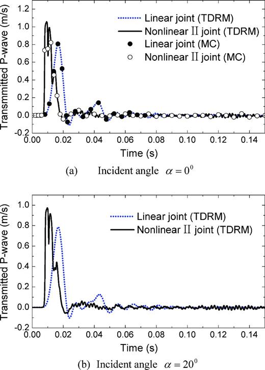
Transmitted P waves based on different methods (incident half-cycle sinusoidal P waves).

Figure 4.

Open in new tabDownload slide

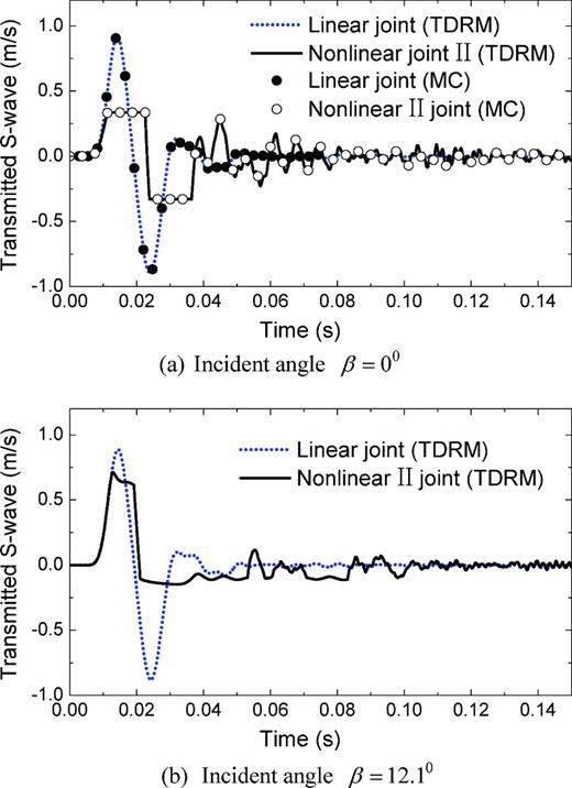
Transmitted S waves based on different methods (incident one-cycle sinusoidal S waves).

The phase shift for wave propagation through a rock between two adjacent joints can be expressed as a time-shifting function, that is, eqs (6) and (7). Unlike for the elastic rock, the wave phase shift for a joint does not satisfy the time-shifting function and is complicated. The arrival times of the transmitted waves shown in Figs 3 and 4 are caused by two-phase shifts, one is for the rocks and the other is for the joints.

Figs 4(a) and (b) show that the relative slip occurs in the non-linear II joints. In Fig. 4(a), the positive and negative slip velocities are equal to each other and both around 0.33 m s^–1, which is equal to the one third of the amplitude of the normally incident S wave. In another word, the ratio of the amplitudes of the incident S wave to the transmitted S wave is equal to the shear strength ratio δ. However, this ratio of the amplitudes in Fig. 4(b) is not limited by δ. The positive slip velocity in Fig. 4(b) is obviously greater than the negative one. This difference is caused by the changes of the compressive normal stress along the joints, when the incident S wave obliquely impinges on the sides of the joints.

Based on the MC and the displacement discontinuity model, Zhao et al. (2006a) derived the wave propagation equation for a set of parallel joints with linear elasticity. Their results for wave propagation across slippery rock joints were also compared with those from UDEC modelling. Zhao et al. (2006b,c) adopted the MC to further analyse the normal incident P- and S-wave propagation across a set of parallel joints with non-linear elasticity and Coulomb-slip behaviour, respectively. Their calculation results are shown as the scattered points in Figs 3(a) and 4(a). By comparison, it is found that the results from the TDRM are identical to the results obtained by the MC.

3.2 Comparison for transmission coefficients

From the wave propagation eqs (8) and (9) and eq. (28), the transmission coefficient can be calculated for an incident P or S wave across a rock joint with linear or non-linear property.

The variation of transmission coefficients with the normalized stiffness of the joint is calculated and shown in Fig. 5, in which the incident P and S waves with harmonic waveform are adopted. The incident angles are α = 20° and β = 12.1° for Figs 5(a) and (b), respectively. In Fig. 5, the continuous curves are calculated by using the TDRM and the scattered points are the results by Gu et al. (1996) for a linear joint. By comparison, it is found that the results from the TDRM for a linear rock joint are consistent with those by Gu et al. (1996).

Figure 5.

Open in new tabDownload slide

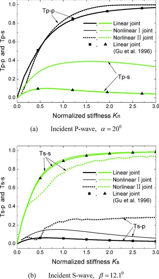
Relationship between transmission coefficients and normalized initial stiffness of the joint.

The relationship between the transmission coefficient and the incident angle is shown in Fig. 6, where the incident P and S waves with the forms of eqs (29) and (30) are adopted, respectively, to analyse wave propagation across a joint with different property.

Figure 6.

Open in new tabDownload slide

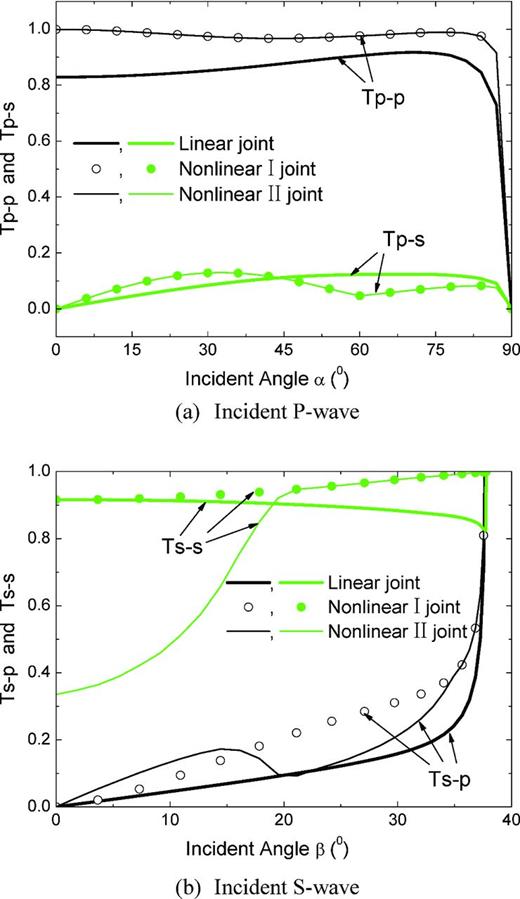
Relationship between transmission coefficient after a single joint and the incident angle.

Figs 5(a) and 6(a) show that the transmission coefficients T_{p − p} for the linear and non-linear joints are quite different, while T_{p − p} of the non-linear I joint is identical to that of the non-linear II joint, so are the transmission coefficients T_{p − s}. Figs 5(b) and 6(b) show that the transmission coefficients, either T_{s − p} or T_{s − s}, for three types of joints, for example, the linear joint, the non-linear I and II joints, are different with each other. The above analysis indicates that wave attenuation across joints is affected by the property of rock joints.

4 PARAMETRIC STUDY AND DISCUSSIONS

The parameters of the rock mass in Section 3 will be taken as the basis for the following investigation. The incident waves have the forms of eqs (29) and (30). This section will focus on the effects of the incident angles α and β, the joint spacing S, the amplitude of incidence and the maximum allowable normal closure d_max on the transmission coefficients.

4.1 Effect of incident angle

Based on the wave propagation eqs (8), (9), (26), (27) and (28), studies on wave propagation across a set of parallel joints with different incident angle for different joint number N are carried out. The calculation results on the transmission coefficients, T_{p − p}, T_{p − s}, T_{s − p} and T_{s − s}, with changes of the incident angle are shown in Figs 7 and 8, for linearly elastic joints and non-linear II joints, respectively.

Figure 7.

Open in new tabDownload slide

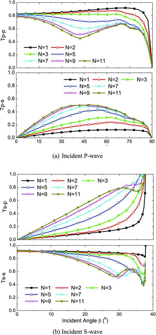
Effect of incident angle on wave propagation across linear joints.

Figure 8.

Open in new tabDownload slide

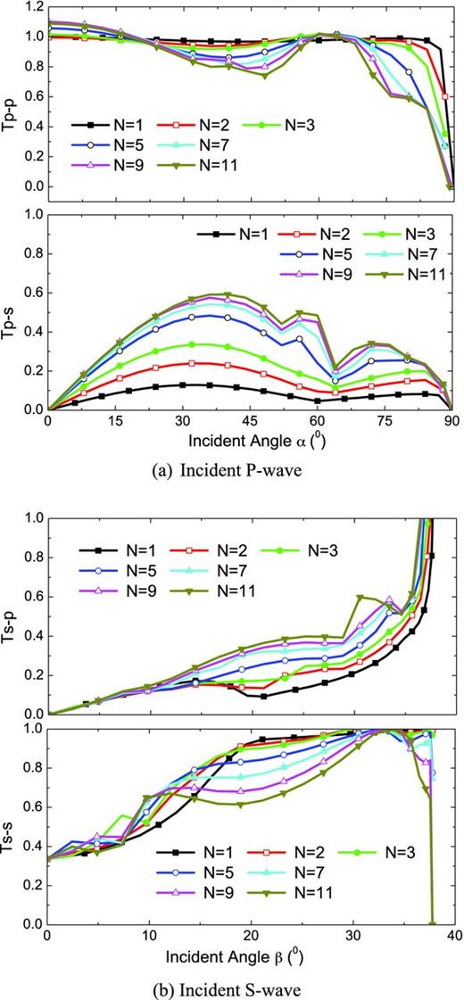
Effect of incident angle on wave propagation across non-linear II joints.

Fig. 7 shows that for a smaller joint number, that is, N is 1, 2 or 3, T_{p − p} and T_{s − s} do not change very much with the incident angle until close to the critical angles of α_c = 90° and β_c = 37.8°. For a larger joint number, that is, N is above 5, T_{p − p} and T_{s − s} decrease obviously with increasing incident angle when α is smaller than 44° or β is smaller than 28°. Fig. 8 shows that, for different joint number N, the transmission coefficient T_{p − p} fluctuates around 1.0 and then drops quickly when α approaches to the critical angle 90°.

It can be seen from Figs 7 and 8 that the transmission coefficients T_{s − s} in two plots are quite different. For example, for β = 0°, T_{s − s} in Fig. 8 is always about 0.33, while T_{s − s} in Fig. 7 is around 0.91 for various joint numbers. The discrepancy is caused by the different joint property. In Fig. 8, T_{s − s} is limited by the shear strength ratio δ when an incident S wave normally propagates across joints with slip behaviour, which can be found in Fig. 4(a). However, there is no such limitation on T_{s − s} for linear joints.

The maximum value of T_{p − s} shown in Figs 7 and 8 divide the area of the incident angle α into two parts: the smaller and larger areas of α. When α is small, T_{p − s} increases with increasing α in both figures. However, when α is large, T_{p − s} in Fig. 7 decreases with increasing α, while the variation of T_{p − s} with α becomes complicated in Fig. 8. This complication is suspected to be related to the friction of joints with Coulomb-slip behaviour. By comparison, it is found that for a given β the transmission coefficient T_{s − p} in Fig. 8 is obviously less than that of Fig. 7 when the joint number N is above 2.

For stress wave propagation across joints with arbitrary incident angle, the normal and shear properties of a joint influence the interaction between the stress wave and the joints. This interaction inversely affects the wave propagation, the transmission and reflection coefficients. Therefore, the effect of the incident angle on the transmission coefficients for linear joints is distinguished from that of non-linear II joints.

4.2 Effect of joint spacing

The variation of transmission coefficient with joint spacing for linear joints has been analysed by Zhao et al. (2011), who used the propagator matrix method to study wave propagation in the frequency domain. In this section, the effect of joint spacing on wave propagation across non-linear II joints is studied for different joint number N, as shown in Fig. 9. The analysis by Zhao et al. (2011) showed that the variation of transmission coefficient T_{p − p} with the change of joint spacing S can be divided into three obvious parts when the joints are linearly elastic. Unlike the results by Zhao et al. (2011), the tendency of T_{p − p} shown in Fig. 9(a) is complicated and fluctuates before it stabilizes to a constant. For six cases of N, Fig. 9(b) shows that the transmission coefficient T_{s − s} increases rapidly to a threshold value first, and then drops to a constant with increasing S.

Figure 9.

Open in new tabDownload slide

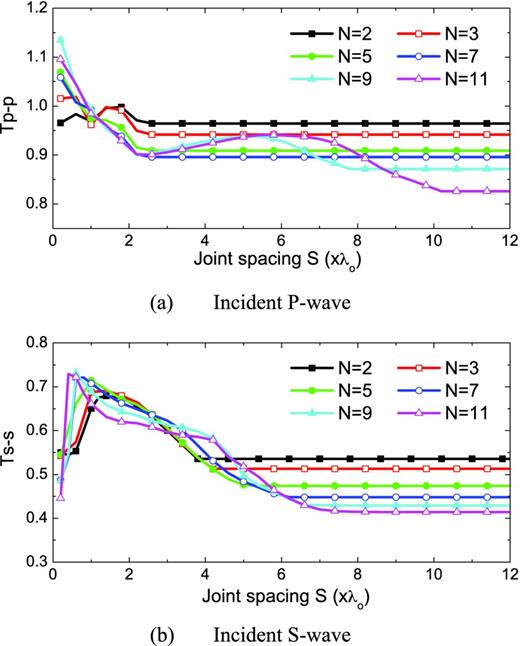
Effect of joint spacing on wave propagation across non-linear II joints.

The joint spacing S at which T_{p − p} and T_{s − s} turn into a constant is defined as the critical value of S. In Fig. 9, the critical value of S for T_{p − p} is 2.6λ₀ for N = 2 and 7.8λ₀ for N = 9, while the critical values of S for T_{s − s} are 3.8λ₀, 5.4λ₀ and 7.4λ₀ for N = 2, 5 and 9, respectively. The constant values of T_{p − p} and T_{s − s} display that the dependence of the transmission coefficients on the joint spacing is not obvious when the joint spacing is larger than its critical value. It further indicates that the multiple reflections between joints have small effects on the transmission coefficients if the joint spacing is sufficiently large.

4.3 Effect of amplitude of incident waves

In the previous study, the initial shear strength τ_s0 is assumed to be | $ \tau _{{\rm s}0} = {{A_{\rm I} z_{\rm s} }/3}$|⁠, where the amplitude of incident waves A_I is 1 m s^–1. In this section, the effect of the incident S-wave amplitude on wave propagation will be studied, given that τ_s0 is | $ {{z_{\rm s} }/3}$|⁠, A_I are 1, 0.6, 0.1 and 0.01 m s^–1 and β = 12.1°.

The calculation results on the magnitude of transmission and reflection coefficients (i.e. T_{s − s} and R_{s − s}) across two joints as a function of the joint spacing S for different A_I are shown in Fig. 10. The normal property of the joints satisfies the B–B model and the shear property exhibits the Coulomb-slip behaviour. It can be observed from Fig. 10 that T_{s − s} is the smallest while R_{s − s} is the biggest for A_I 1 m s^–1. When A_I are 0.1 and 0.01 m s^–1, T_{s − s} and R_{s − s} are close to each other for two values of A_I. Except the zone for the smaller joint spacing, that is, S ≤ 0.75λ₀, T_{s − s} for A_I = 0.6 m s^–1 is smaller than those for A_I = 0.1 and 0.01 m s^–1. It is found from Fig. 4(b) that for an oblique S-wave incidence, the relative slip may appear for the joints when A_I is larger than | $ {1/3}$| m s^–1. The amplitude of the transmitted wave after slippery joints attenuates more than that for joints without slippery behaviour. Hence, T_{s − s} for A_I = 0.1 and 0.01 m s^–1 are obviously larger than T_{s − s} for A_I = 1.0 and 0.6 m s^–1, while it is the opposite for R_{s − s}.

Figure 10.

Open in new tabDownload slide

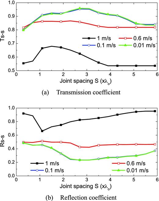
Effect of amplitude of incident waves on S wave propagation across non-linear II joints.

For a normal incident P wave with A_I 1 m s^–1, the maximum value of σ_d on the left-hand side of the first joint is equal to ρc_p. For oblique incident P or S waves, the maximum value of σ_d is affected by the incident angle. If |(σ₀ + σ_d) · tan φ/k_s| ≥ u_s, slip failure appears, where σ₀ is the geostress and equal to z_s/(3tan φ) in this section.

4.4 Effect of joint maximum allowable normal closure

The results on T_{p − p} and T_{s − s} as functions of the maximum allowable normal closure d_max for different joint number N are shown in Fig. 11, where α and β are 20° and 12.1° for incident P and S waves, respectively. Fig. 11(a) shows that the transmission coefficient T_{p − p} for wave propagation across a single joint decreases with increasing d_max. When d_max is larger, the joint with the B–B model is softer, which results in smaller T_{p − p} across a single joint. In Fig. 11(a), T_{p − p} achieves a maximum value when d_max is around 3 mm for N of 2–7 and 4 mm for N of 9 and 11. Then T_{p − p} decreases in amplitude when d_max further either increases or decreases. It is also found from Fig. 11(a) that for a given range of d_max, T_{p − p} is greater with a larger joint number N. This indicates that the effect of multiple wave reflections among joints on the amplitude of the transmitted P wave is more significant when the joint number is larger.

Figure 11.

Open in new tabDownload slide

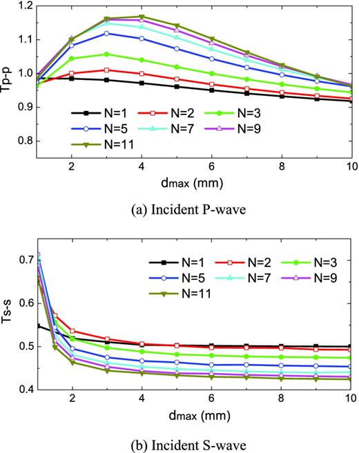
Effect of joint maximum allowable normal closure d_max on wave propagation.

Fig. 11(b) shows that T_{s − s} drops sharply with d_max initially, that is, d_max smaller than 2 mm, and decreases slightly with increasing d_max for all the cases with N ranging from 2 to 11. Therefore, the effect of d_max on T_{s − s} is not obvious when d_max is large or when the joint is soft.

5 CONCLUSIONS AND DISCUSSIONS

The TDRM is developed to study wave propagation across non-linear and slippery rock joints in this paper. Both incident P and S waves obliquely impinge on the joints. According to the stress and displacement field around a joint, the interaction between the waves and the joint is analysed. The wave propagation equation is then established in the time domain. The equation includes two modes, one is the elastic mode and the other is the slippery mode. The method can be applied to any choice of wavelength.

As the analysis is carried out in the time domain, the TDRM is more efficient for incidence with any waveform compared to other mathematical methods, such as the Fourier and inverse Fourier transform. By comparison with the existing methods for some specific cases, the TDRM is proved to be effective to study wave propagation across a set of parallel joints with non-linear property.

For normal and oblique cases, calculation for wave propagation across rock joints is conducted when the joints are linearly elastic, non-linearly elastic and slippery, respectively. By comparison, it is found that the wave propagation across a single joint or multiple joints is influenced by the normal and shear properties of the joints.

Parametric studies show that the incident angle, the joint spacing, the amplitude of incidence and the joint maximum allowable normal closure all affect wave propagation across multiple joints, such as the transmitted waveform, the transmission and reflection coefficients.

It is noted that the coupling effect for the normal and shear properties of joints is not considered in this study. In addition, the TDRM cannot deal with the case for the stress wave with a curved wave front. Further exploration is underway to extend the current method for more complicated properties of joints and incident waves.

The author acknowledges the support of Chinese National Science Research Fund (41272348, 11072257, 51025935, 51174190) and the Major State Basic Research Project of China (2010CB732001). The author also thanks Prof Jian Zhao of EPFL Switzerland for his discussion and review of this paper.

REFERENCES

APPENDIX

Fig. A1 shows the interaction between a joint and four waves, that is, right-running (RR) and left-running (LR) P waves, right-running (RR) and left-running (LR) S waves.

Figure A1.

Open in new tabDownload slide

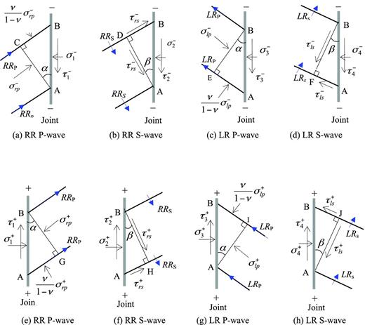
Stress wave interaction with two sides of a joint.