-
PDF
- Split View
-
Views
-
Cite
Cite
Shin'ichiro Ando, Aurélien Benoit-Lévy, Eiichiro Komatsu, Angular power spectrum of galaxies in the 2MASS Redshift Survey, Monthly Notices of the Royal Astronomical Society, Volume 473, Issue 4, February 2018, Pages 4318–4325, https://doi.org/10.1093/mnras/stx2634
Close - Share Icon Share
Abstract
We present the measurement and interpretation of the angular power spectrum of nearby galaxies in the 2MASS Redshift Survey catalogue with spectroscopic redshifts up to z ≈ 0.1. We detect the angular power spectrum up to a multipole of ℓ ≈ 1000. We find that the measured power spectrum is dominated by galaxies living inside nearby galaxy clusters and groups. We use the halo occupation distribution (HOD) formalism to model the power spectrum, obtaining a fit with reasonable parameters. These HOD parameters are in agreement with the 2MASS galaxy distribution we measure towards the known nearby galaxy clusters, confirming validity of our analysis.
1 INTRODUCTION
The 2MASS Redshift Survey (2MRS; Huchra et al. 2012) is a spectroscopic follow-up of galaxies detected in the photometric Two Micron All Sky Survey (2MASS; Skrutskie et al. 2006). The 2MRS provides an excellent probe of the nearby distribution of galaxies up to z ≈ 0.1. Among many applications of this full-sky map of galaxies, one powerful application is the cross-correlation with a map of different tracers with unknown redshifts.
For example, the cross-correlation of the photometric 2MASS galaxies with the cosmic microwave background (CMB) temperature map was used to measure a dynamical signature of dark energy in the CMB via the integrated Sachs–Wolfe effect (Afshordi, Loh & Strauss 2004). The cross-correlation with a gamma-ray map measured by Large Area Telescope (LAT) of the Fermi satellite has an excellent sensitivity to gamma-rays from annihilation of dark matter particles (Xia et al. 2011; Ando et al. 2014; Cuoco et al. 2015). The cross-correlation of the 2MRS catalogue with a map of the thermal Sunyaev–Zeldovich effect derived from the Planck data (Planck Collaboration XXII 2016a) has been measured recently (Makiya et al., in preparation), and it tells us how hot gas traces galaxies in the nearby Universe.
To understand properly various such measurements of cross-correlations, we must understand clustering of galaxies in the 2MRS catalogue, i.e. the auto power spectrum of 2MRS. In this paper, we present the measurement and interpretation of the 2MRS angular power spectrum. Frith, Outram & Shanks (2005) presented the angular power spectrum of the 2MASS full release extended source catalogue.
Throughout this paper, we adopt cosmological parameters of Planck Collaboration XIII (2016b, table 4, TT+lowP+lensing). We define a halo mass (M ≡ Mvir) as a mass enclosed within a virial radius rvir, within which the average matter density is Δvir(z) times the critical density ρc(z), where Δvir(z) ≡ 18π2 + 82d − 39d2 with |$d \equiv \Omega _{\rm m}(1+z)^3/[\Omega _{\rm m}(1+z)^3+\Omega _\Lambda ]-1$| (Bryan & Norman 1998). Conversion from other definitions of the mass (such as M200 defined with radius r200 within which the average density is 200 times the critical density) is done by assuming a Navarro–Frenk–White (NFW) density profile (Navarro, Frenk & White 1997) and using fitting formulae given in Hu & Kravtsov (2003).
2 ANGULAR POWER SPECTRUM
2.1 Construction of the galaxy density map
We avoid regions close to the Galactic plane by masking pixels in |b| < 5° for 30° < l < 330° and |b| < 10° otherwise. In addition, we mask small regions that have very low redshift completeness as computed by Lavaux & Hudson (2011) (the white regions in the left-hand panel of their Fig. 4). The fraction of sky available for the analysis is fsky = 0.877.
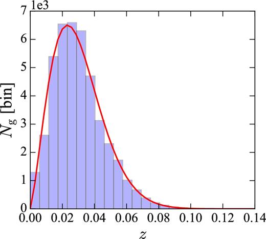
The number of 2MRS galaxies in each redshift bin, compared with the fitting functon, equation (2).
Redshifts of the 2MRS are claimed to be complete for galaxies up to a magnitude of Ks = 11.75, and are nearly volume-limited up to z ≈ 0.02. Completeness of redshifts as computed by Lavaux & Hudson (2011) is quite homogeneous except small regions that have very low completeness. We mask those regions as described above, and apply no completeness correction for the derived δg.
2.2 Estimation of the angular power spectrum
We used the publicly available software polspice2 to estimate the angular power spectrum of δg. polspice allows for an efficient de-convolution of the harmonic couplings induced by the mask.
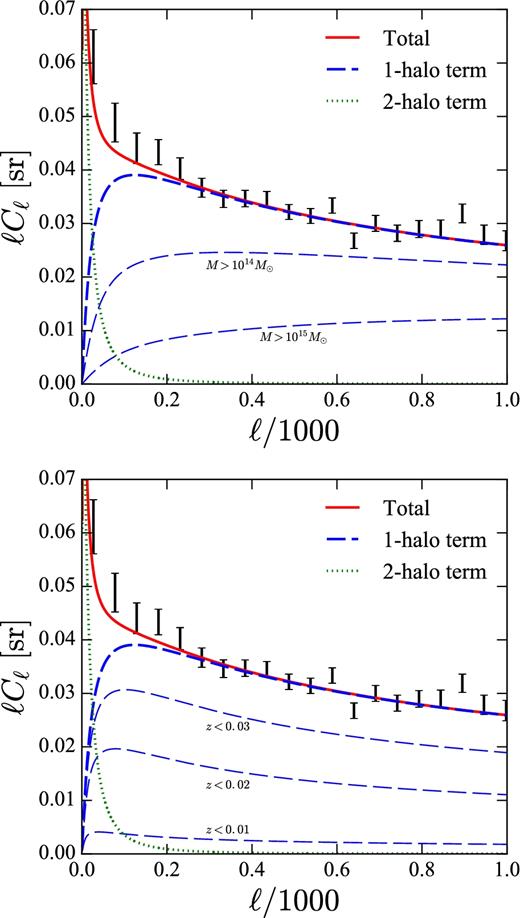
We present the measured power spectrum minus the noise power in Fig. 2. We detect the power spectrum clearly all the way to the maximum multipole reliably resolved by the healpix map with Nside = 512, i.e. ℓmax = 2Nside = 1024. This indicates that the 2MRS galaxies are strongly clustered: We have 43 182 galaxies over 87.7 per cent of the sky, and thus the mean galaxy number density is only 1.2 deg−2. As we show in this paper, many of the 2MRS galaxies reside in galaxy clusters and groups, producing power at multipoles much higher than that of the mean separation of galaxies.
Angular power spectrum of the 2MRS galaxies, compared with the best-fitting model (solid; see Section 3). The one- and two-halo terms are shown as the thick dashed and the dotted curves, respectively. The thin dashed curves show contributions from mass ranges relevant for clusters of galaxies as indicated (top panel), and those from a few different redshift ranges (bottom panel). The error bars show the diagonal elements of the covariance matrix (see Section 2.3).
We tabulate the measured power spectrum data with diagonal elements of the covariance matrix in Table 1.
Power spectrum of the 2MRS, the Gaussian variance and the total variance.
| Mean multipole . | Multipole range . | ℓCℓ (10−2 sr) . | |$\sqrt{\mbox{Cov}(\ell C_\ell ,\ell C_\ell )_{\rm Gauss}}$|(10−2 sr) . | |$\sqrt{\mbox{Cov}(\ell C_\ell ,\ell C_\ell )}$| (10−2 sr) . |
|---|---|---|---|---|
| 27 | 2 ≤ ℓ < 53 | 6.11 | 0.32 | 0.50 |
| 78 | 53 ≤ ℓ < 104 | 4.88 | 0.12 | 0.36 |
| 129 | 104 ≤ ℓ < 155 | 4.40 | 0.10 | 0.29 |
| 180 | 155 ≤ ℓ < 206 | 4.33 | 0.10 | 0.24 |
| 231 | 206 ≤ ℓ < 257 | 4.03 | 0.10 | 0.20 |
| 282 | 257 ≤ ℓ < 308 | 3.67 | 0.10 | 0.18 |
| 333 | 308 ≤ ℓ < 359 | 3.46 | 0.10 | 0.16 |
| 384 | 359 ≤ ℓ < 410 | 3.47 | 0.11 | 0.15 |
| 435 | 410 ≤ ℓ < 461 | 3.45 | 0.11 | 0.15 |
| 487 | 461 ≤ ℓ < 513 | 3.22 | 0.11 | 0.14 |
| 538 | 513 ≤ ℓ < 564 | 3.14 | 0.12 | 0.14 |
| 589 | 564 ≤ ℓ < 615 | 3.33 | 0.12 | 0.14 |
| 640 | 615 ≤ ℓ < 666 | 2.68 | 0.13 | 0.14 |
| 691 | 666 ≤ ℓ < 717 | 3.00 | 0.14 | 0.15 |
| 742 | 717 ≤ ℓ < 768 | 2.82 | 0.14 | 0.15 |
| 793 | 768 ≤ ℓ < 819 | 2.90 | 0.15 | 0.16 |
| 844 | 819 ≤ ℓ < 870 | 2.90 | 0.16 | 0.16 |
| 895 | 870 ≤ ℓ < 921 | 3.19 | 0.17 | 0.17 |
| 946 | 921 ≤ ℓ < 972 | 2.79 | 0.18 | 0.18 |
| 998 | 972 ≤ ℓ < 1024 | 2.68 | 0.18 | 0.19 |
2.3 Covariance matrix
We shall describe details of the computation of |$T_{\ell \ell ^{\prime }}$| in Section 4.1, and only outline our procedure here. As the trispectrum term depends on the model of the power spectrum itself, we cannot calculate |$T_{\ell \ell ^{\prime }}$| a priori. Thus, we first determine the model parameters using the Gaussian covariance in the likelihood analysis. We then calculate |$T_{\ell \ell ^{\prime }}$| for the best-fitting model parameters, and re-determine the model parameters using the sum of the Gaussian term and |$T_{\ell \ell ^{\prime }}$| in the likelihood. The error bars shown in Fig. 2 are the diagonal elements of the total covariance matrix including the trispectrum term.
The square-root of the diagonal elements of the Gaussian and total covariance matrices are reported in Table 1.
3 MODEL
3.1 Halo model
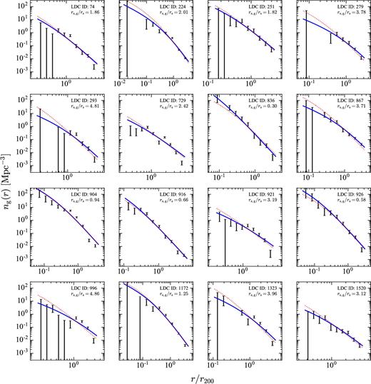
The best-fitting values for the ratio of the scale radius of galaxies to that of dark matter rg, s/rs vary across clusters. We use the mass–concentration relation of Sánchez-Conde & Prada (2014) to compute rs as a function of halo masses, which are inferred from dynamical analysis of the member galaxies in each cluster (Crook et al. 2007, 2008). The solid curves in Fig. 3 show NFW profiles with the best-fitting rs, g/rs from unbinned likelihood analysis. Since the parameter rs, g/rs varies from cluster to cluster, and the cluster mass estimates as well as intrinsic scatter in the mass–concentration relation are uncertain, we shall treat it as a free parameter.
3.2 Halo occupation distribution
We do not vary the HOD parameters as a function of z. In principle, this approximation may break down for a magnitude-limited sample such as the 2MRS, as the dominant galaxy population may change depending on z. As the 2MRS is nearly volume-limited up to z ≈ 0.02, it is safe to use the HOD up to that redshift; however, we need to be careful when interpreting the HOD parameters derived from the whole sample. We shall come back to this point later.
4 RESULTS AND INTERPRETATION
4.1 Posterior distribution of the model parameters
Medians and 1σ credible intervals of the posterior distributions of the model parameters, for three independent runs of computing the angular power spectrum. The second row shows the prior range, within which each parameter was drawn from a flat distribution. The last column shows |$\chi _{\rm min}^2$| compared with a degree of freedom (dof).
| Catalogue . | rmax, g/r200 . | rs, g/rs . | log (Mmin/M⊙) . | log (M1/M⊙) . | α . | |$\chi _{\rm min}^2 / {\rm dof}$| . |
|---|---|---|---|---|---|---|
| Prior | 0–15 | 0–15 | 9–14 | 9–14 | 0–2 | |
| Run 1 | |$6.9^{+3.0}_{-1.7}$| | |$0.62^{+0.13}_{-0.12}$| | |$11.84^{+0.17}_{-0.14}$| | |$11.98^{+0.18}_{-0.24}$| | |$0.849^{+0.073}_{-0.088}$| | 33.3/16 |
| Run 2 | |$6.4^{+3.1}_{-1.6}$| | |$0.72^{+0.15}_{-0.14}$| | |$11.87^{+0.19}_{-0.17}$| | |$11.97^{+0.21}_{-0.27}$| | |$0.855^{+0.087}_{-0.096}$| | 29.7/16 |
| Run 3 | |$6.7^{+2.5}_{-1.5}$| | |$0.61^{+0.11}_{-0.10}$| | |$11.83^{+0.15}_{-0.13}$| | |$11.97^{+0.17}_{-0.21}$| | |$0.837^{+0.068}_{-0.074}$| | 47.2/16 |
We use the Markov chain Monte Carlo (MCMC) to explore the parameter space. To this end, we use the multinest (Feroz & Hobson 2008; Feroz, Hobson & Bridges 2009; Feroz et al. 2013) package for the MCMC and obtain the posterior distributions of the model parameters.
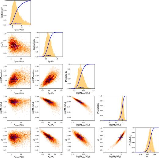
Since we estimate the noise contribution to the power spectrum by randomly dividing the 2MRS catalogue into two (see Section 2.2), the galaxy density field used for computing the power spectrum contains some randomness. To quantify the impacts of this randomness, we calculated three sets of density fields with different initial random seeds, and repeated the parameter estimation. The power spectrum shown in Fig. 2 is the first set ‘run 1’, whose posterior distribution of the parameters is shown in Fig. 4. The posterior distributions for ‘run 2’ and ‘run 3’ are similar. The parameter values are summarized in Table 2. We find that all runs give similar results.
Posterior distribution of the model parameters. The diagonal panels show the one-dimensional distribution marginalized over the other parameters as well as the cumulative distribution (line). The other panels show the two-dimensional marginalized joint distributions. The cross symbols show the mean and the 1σ uncertainty.
In the top panel of Fig. 2, we show the contributions from different ranges of halo masses. We find that the angular power spectrum is dominated by the one-halo term at ℓ ≳ 30. In other words, the 2MRS angular power spectrum is dominated by galaxies residing in nearby galaxy clusters and groups.
The derived HOD parameters (Table 2) are reasonable: the galaxy distribution extends out to several times r200; the galaxy and dark matter scale radii are similar on average, with a slight preference for rs, g/rs < 1, though this parameter varies significantly across individual haloes (see Fig. 3); the mass scales enter into the HOD are of the order of the Milky Way mass; and the number of satellite galaxies increases with the host halo mass slightly slower than a linear relation.
The best-fitting models give |$\chi _{\rm min}^2 = -2 \ln \mathcal {L}_{\rm max}=33.3$|, 29.7 and 47.2 for 16 degrees of freedom (i.e. 21 data points and 5 parameters) for runs 1–3. Taken at the face values, the probabilities to exceed (PTE) these |$\chi ^2_{\rm min}$| are 6.7 × 10⁻³, 2.0 × 10⁻² and 6.3 × 10⁻⁵. These PTE are rather low, except for run 2. This may suggest that our HOD modelling is too simplistic, requiring more sophisticated ones instead. For example, as we stated in Section 3.2, the use of the HOD model for a magnitude-limited sample would introduce an error. (The 2MRS is nearly volume-limited up to z ≈ 0.02.) Such modelling error would not only affect the model power spectrum, but also the covariance matrix via the trispectrum term, potentially changing a χ2 value. None the less, the model presented here will probably be good enough for interpreting various cross-correlation results.
4.2 Contribution from the known galaxy groups and clusters
Fig. 2 shows contributions from the mass ranges relevant for clusters of galaxies: M > 1014 and >1015 M⊙. We find that most of the power at small angular scales can be attributed to galaxies residing in galaxy clusters. We can test this result directly by summing up the contributions from galaxy groups and clusters we see in the 2MRS. We use recent group catalogues of 2MRS by Tully (2015b) and Lu et al. (2016).
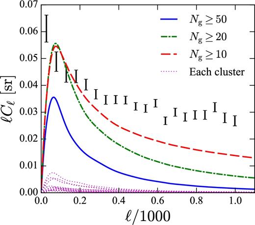
Angular power spectrum of galaxies residing in groups and clusters detected in the 2MRS. The cumulative contributions from groups and clusters above a certain size are shown as the solid (Ng ≥ 50), dot–dashed (Ng ≥ 20) and dashed (Ng ≥ 10) curves. There are 17, 78 and 299 groups and clusters containing 1578, 3376 and 6217 galaxies in these samples, respectively. The dotted curves show Cℓ from each of the 17 largest clusters.
We also show individual contributions from the 17 largest clusters. We find that about ten per cent of the power in sub-degree angular scales comes from these 17 clusters that host more than 50 member galaxies. The remaining power comes from hundreds of galaxy groups and clusters. For smaller groups, the approximation used in equation (18) becomes less valid, because one can no longer regard the galaxy distribution as given by the smooth NFW function. None the less, Fig. 5 provides a useful cross-check of our result.
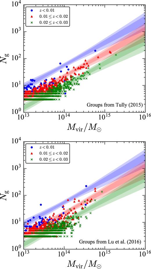
In the top panel of Fig. 6, we show the numbers of member galaxies found in each group or cluster in the Tully (2015b) catalogue as a function of its virial mass Mvir. We estimate the virial mass of the groups and clusters through equation (4) of Tully (2015a) and a proper conversion from M200 to Mvir afterwards. We also show the 68 per cent and 95 per cent credible intervals for the mean galaxy number, 〈Ng|M〉 ≡ 〈Ncen|M〉 + 〈Nsat|M〉, from the posterior distribution of the HOD parameters of ‘run 1’. The bottom panel of Fig. 6 shows the same, but for an independent 2MRS group catalogue by Lu et al. (2016).
Numbers of member galaxies in groups and clusters of galaxies in the Tully (2015b, top) and Lu et al. (2016, bottom panel) catalogues. Different symbols show different redshift ranges. The thick and thin bands are the 68 per cent and 95 per cent credible intervals for the mean galaxy number predicted by the HOD model, 〈Ng|M〉, after the selection effect has been corrected for each of these three subsamples (see the text).
The HOD parameters are intrinsic to the galaxies. To compare with the observation, we correct for the selection effect as follows. The number density of the observed galaxies is estimated from the redshift distribution [equation (2)] as |$n_{\rm 2MRS}(z) = (\text{d}N_{\rm g}/\text{d}z)(\text{d}\chi /\text{d}z)^{-1}/(4\pi f_{\rm sky} \chi ^2)$|, while the intrinsic density is given by nHOD(z) = 〈ng(z)〉 from equation (9). In Fig. 6, for each of the three subsamples (with mean redshifts of |$\bar{z} = 0.0065, 0.016$| and 0.025 for Tully 2015b and |$\bar{z} = 0.0067, 0.016$| and 0.025 for Lu et al. 2016), we re-scale the total number of member galaxies 〈Ng|M〉 by |$n_{\rm 2MRS}(\bar{z}) / n_{\rm HOD}(\bar{z})$|. We see very good agreement between the HOD model and the observation of the groups and clusters, justifying our model.
5 CONCLUSION
We have presented the measurement and interpretation of the angular power spectrum of the 2MRS. We found that the 2MRS galaxies are so highly clustered that the power spectrum at ℓ ≳ 30 is dominated by the one-halo term, i.e. galaxies residing in nearby galaxy groups and clusters. We demonstrated this by the HOD modelling of the power spectrum, as well as by directly summing up the contributions from groups and clusters identified in the 2MRS catalogue.
This property makes the 2MRS catalogue well suited for cross-correlation studies with other tracers of groups and clusters, for example, hot gas traced by the thermal Sunyaev–Zeldovich effect (Makiya et al., in preparation), gamma-rays from annihilation of dark matter particles in sub-haloes of groups and clusters (Ando et al. 2014), and so on. Properly interpreting such cross-correlation measurements requires accurate information of clustering statistics of the 2MRS galaxies, and our measurement and HOD model provide the required information.
Acknowledgements
We thank Lucas Macri for providing us with the 2MRS catalogue. This work was supported by the Netherlands Organization for Scientific Research (NWO) through Vidi grant (SA), and also in part by JSPS KAKENHI Grants, JP15H05896 (EK) and JP17H04836 (SA). We acknowledge the use of healpix (Górski et al. 2005) and polspice (Szapudi, Prunet & Colombi 2001) packages.
The maximum radius rmax, g depends on how one defines galaxy clusters. In a more recent catalogue of Tully (2015b), clusters are defined to be more compact than the LDC definition of Crook et al. (2007, 2008), yielding smaller values of rmax, g/r200. In order to accommodate this ambiguity, we shall treat rmax, g/r200 as a free parameter.
REFERENCES


