


Abstract
The extremely regular, periodic radio emission from millisecond pulsars makes them useful tools for studying neutron star astrophysics, general relativity, and low-frequency gravitational waves. These studies require that the observed pulse times of arrival be fitted to complex timing models that describe numerous effects such as the astrometry of the source, the evolution of the pulsar's spin, the presence of a binary companion, and the propagation of the pulses through the interstellar medium. In this paper, we discuss the benefits of using Bayesian inference to obtain pulsar-timing solutions. These benefits include the validation of linearized least-squares model fits when they are correct, and the proper characterization of parameter uncertainties when they are not; the incorporation of prior parameter information and of models of correlated noise; and the Bayesian comparison of alternative timing models. We describe our computational setup, which combines the timing models of tempo2 with the nested-sampling integrator multinest. We compare the timing solutions generated using Bayesian inference and linearized least-squares for three pulsars: B1953+29, J2317+1439, and J1640+2224, which demonstrate a variety of the benefits that we posit.
INTRODUCTION
With spin periods as stable as a part in 1015 over years, millisecond pulsars are exceedingly regular rotators, and their periodic radio pulses can be timed with sub-μs accuracy (Verbiest et al. 2008), making pulsars great laboratories to study neutron star astrophysics, to test general relativity (Kramer et al. 2006; Antoniadis et al. 2013; for a review, see Stairs 2003), and to serve as quasi-ideal clocks in searches for gravitational waves (GWs; Sazhin 1978; Detweiler 1979). The most sensitive GW searches proceed by correlating the unexplained residuals in the timing series of multiple pulsars in a pulsar-timing array (PTA; Hellings & Downs 1983). Recent years have seen a renewed interest in this effort, with the formation of three major regional programmes [the EPTA (van Haasteren et al. 2011), NANOGrav (Demorest et al. 2013), and the PPTA (Shannon et al. 2013)], which have now joined into a global collaboration to share data and expertise (Hobbs et al. 2010).
A large part of the science enabled by pulsars unfolds through a rather pure instance of model fitting: pulsar astronomers build complex, many-parameter mathematical models of pulsar-spin evolution and radio-pulse propagation out of the pulsar system (which is often a close binary), through interstellar space, across the Solar system, and into our large radio dishes and broad-band receivers. These timing models must include not only the basic geometry of light propagation, but also the effects of gravity, relativity, binary companions, and more. They must also predict the times of arrival (TOAs) of every single pulse (out of hundreds of millions across years of observation, although only a subset of pulses are actually timed) within a fraction of a period (Edwards, Hobbs & Manchester 2006; Lommen & Demorest 2013). It is no wonder then that such a painstaking, all-encompassing effort should yield physical measurements of great precision, although one may wonder that nature would be so kind to gift such excellent toys to astronomers!
In practice, model fitting must be preceded by the proper calibration of the data and by the mitigation of systematic effects, both of which are major areas of research (see Lommen & Demorest 2013 for some references). One interesting twist is that timing models must be bootstrapped, since pulses from millisecond pulsars are not detectable individually, but must be ‘folded’ in batches of hundreds or thousands, requiring a basic (but already accurate) model to align the folding. Another twist is that for arguably the most promising GW source for PTAs, the stochastic background from the ensemble of massive black hole binaries at the centres of galaxies (Sesana 2013), the signal of interest is the noise-like residual that is left after subtracting the deterministic timing model, which can only be characterized statistically. Luckily, the GW background is distinguished from other sources of noise by appearing in correlated fashion for all the pulsars in the array (Hellings & Downs 1983).
After the pulsar data sets are distilled (by way of rather sophisticated processing) into sets of TOAs, the estimation of pulsar parameters is routinely performed by solving for the maximum-likelihood timing model using linear least squares (Press et al. 1992, ch. 15), as implemented in the widely adopted pulsar-timing software packages tempo (Manchester et al. 1998) and tempo2 (Edwards et al. 2006; Hobbs & Edwards 2006, Hobbs, Edwards & Manchester 2006; Hobbs et al. 2009). These packages are impressive accomplishments in the complexity and precision of their timing models, but they offer only rather straightforward fitting options.
The main limitation of linear least-squares maximum-likelihood estimation is that it is a local technique that relies on linearizing the model of interest with respect to a vector of parameter corrections. This does not keep the technique, in most practical cases, from finding global maxima by chaining a sequence of local corrections. It does however mean that the linear approximation must be accurate at least across the parameter ranges returned as uncertainties by the least-squares process itself – otherwise, the reported uncertainties are certain to be unreliable. Thus, the risk is that the impressive accuracy claimed in some pulsar-timing ephemerides could be overstated, especially for poorly constrained parameters.
The other limitation of the standard approach does not concern the mathematical technique itself, but rather its physical boundary conditions. Least-squares timing-model fits are usually set up by assuming that the only source of error in the TOAs is radiometer noise, which can be estimated directly from the raw data (more in Section 2), and which is taken to be Gaussian and uncorrelated. However, for certain pulsars, these errors appear to be too large or too small (i.e. within the logic of least-squares estimation, they lead to very small or very large χ2 values), thus, skewing uncertainty estimates. Other pulsars show hints of residual correlated noise with ‘red’ spectra dominated by low-frequency components (Cordes & Shannon 2010; Shannon & Cordes 2010; Coles et al. 2011; van Haasteren & Levin 2013), which is not taken into account in the standard estimation process. Even the very presence of GWs could conceivably bias parameter estimation.1
In this paper, we argue that all these concerns can be addressed by a fully non-linear Bayesian-inference approach (Gregory 2010) that derives distributions (rather than point estimates) for the pulsar-timing parameters by sampling freely across parameter space, and computing the full timing model at each point. Furthermore, we argue that this approach offers additional scientific opportunities (listed below), and that it is both practical and computationally feasible with current hardware resources and software components. As an example, in Section 4, we present Bayesian analyses of three NANOGrav pulsars (Demorest et al. 2013), which we performed by using tempo2 as a library to form timing residuals for arbitrary pulsar parameter sets, and by calling it from a popular stochastic sampler [the nested-sampling (Skilling 2004) package multinest (Feroz, Hobson & Bridges 2009)].
Our experience leads us to advocate for a broad use of full Bayesian inference in timing-model studies, because of the following benefits.
Uncertainties. Bayesian inference offers reliable estimates of parameter uncertainties (as the moments or quantiles of marginalized posteriors) and parameter correlations (as the joint marginalized posteriors). These estimates fully take into account the non-linear functional dependence of the model on the parameters. The least-squares formalism can reproduce these estimates only in the infinite signal-to-noise limit where all parameters have normal error distributions around their maximum-likelihood values.
Priors. Bayesian inference allows the statistically principled incorporation of prior knowledge about some of the parameters. For instance, Madison, Chatterjee & Cordes (2013) argue that pulsar positions and proper motions determined from VLBI astrometry can substantially improve timing-model determinations. In our worked-out examples of Section 4, we use estimates of distance from dispersion measurements as priors for the parallax, a poorly determined parameter that can even take unphysical negative values in least-squares estimation.
Noise. Bayesian inference lets us solve simultaneously for the timing-model parameters and for the noise parameters that describe the errors in the timing data, obtaining joint probability distributions for both. As discussed by van Haasteren & Levin (2013), we may model the errors as containing a white, uncorrelated noise component (perhaps with extra parameters that modulate the empirical estimates of radiometer noise) but also any number of red, correlated Gaussian processes (Rasmussen & Williams 2005).
Model comparison. Bayesian inference lets us compare and choose between alternative timing+noise models with different parameter ranges or components, by evaluating the relative model evidence (Gregory 2010). The comparison may be, for instance, between a white-noise and white+red-noise model, two different descriptions of binary dynamics, or even the dynamics of general relativity and that of a modified theory of gravity [as advocated by Del Pozzo, Veitch & Vecchio (2011) for GW measurements].
We note one last benefit: we can use non-linear Bayesian inference to validate the results of least-squares, maximum-likelihood estimation, which by itself does not offer the means for such a validation, but which will undoubtedly remain the workhorse in this field. Such validation is necessary also for the noise-estimation and GW-search methods that marginalize the posterior over the timing-model parameters by assuming that the residuals can be accurately represented as linearized functions (van Haasteren et al. 2011); we shall say more about these methods in Section 2.
We are not the first to suggest that Bayesian methods can be applied to pulsar timing. Messenger et al. (2011) propose two Bayesian methods to generate TOAs from raw and folded radio data – that is, to perform the data-analysis step prior to timing-model fitting. They also discuss the possibility of an end-to-end Bayesian analysis. Independently from and simultaneously with our work, Lentati et al. (2014) developed a software package, based on the very same two components that we use, to perform a joint Bayesian analysis of the non-linear pulsar-timing model and of any stochastic components. They emphasize that the concurrent modelling of correlated noise (in addition to uncorrelated time-of-arrival errors) can change the estimates and uncertainties of timing-model parameters very significantly; working with simulated and real pulsar data, they show examples of non-normal parameter posteriors in observations with low signal-to-noise ratio, and they compare the Bayesian evidence of different noise models and different subsets of timing-model parameters. We agree with most of the theoretical framework laid out in Lentati et al. (2014), but we differ on the proper treatment of Bayesian-model comparison, as we discuss in greater detail in Section 5.
The rest of this paper is organized as follows. In Section 2, we present an overview of pulsar-timing-model fitting of both least squares and Bayesian flavours, and explain how the latter overcomes the shortcomings of the former. In Section 3, we describe our computational setup and in Section 4, we recount our three case studies of Bayesian-model fitting. Lastly, in Section 5, we offer our conclusions and recommendations.
AN OVERVIEW OF PULSAR TIMING AND MODEL FITTING
While it is useful to think of pulsars as ideal clocks for the purpose of GW detection, there are actually several experimental steps that separate the emission of radio pulses from the analyses that can determine pulsar parameters and to search for GWs. Lorimer (2008) and Lommen & Demorest (2013) give thorough accountings of all the steps involved, which we summarize in this section to provide context for our later discussion. In this section, we also develop the basic mathematical formalism needed for standard (i.e. least squares) and Bayesian-model fitting.
Times of arrival
After the pulses are emitted, they traverse the interstellar medium and are received at the radio telescope, where they are usually observed at central frequencies ∼1 GHz, with bandwidths of tens to hundreds of MHz. The radio signals are then de-dispersed and folded: that is, because the pulses are too weak to be analysed individually, they are aligned (requiring a basic fiducial set of pulsar parameters) and added together. For many pulsars, the resulting average pulse shapes have remarkably stable profiles across observing epochs, so they allow the accurate determination of pulse TOAs. These are defined as the timestamps of a fiducial point on the profile, such as its maximum, referred to a (notional) individual pulse at the beginning or at the mid-point of each observation (Lommen & Demorest 2013). In effect, TOAs are determined by cross-correlating the observed profiles with an analytical or empirical ‘template.’
TOA errors
The resulting TOA uncertainty is roughly the width of the profile, divided by signal-to-noise ratio (SNR) of the observation. These errors are usually idealized as Gaussian, uncorrelated noise (known as radiometer noise), although the variation of profiles with time and across the observation bandwidth has the potential of introducing systematic components. Furthermore, for some pulsars and observations, the correlation uncertainties appear to be systematically over- or underestimated; as a result, observers introduce ad hoc corrections to multiply the uncertainties by a constant factor (EFAC) or to postulate additional uncorrelated noise (EQUAD; Lommen & Demorest 2013).
Timing model
The regularity of pulsar emission becomes evident only after the topocentric TOAs |$t_i^\mathrm{obs}$| are transformed to the pulsar frame by subtracting a number of systematic propagation delays (Edwards et al. 2006). Working back from the observatory to the pulsar, these delays include:
the transformation from the observatory frame to the Solar system-barycentre (SSB) frame, which involves clock corrections to a fiducial terrestrial time standard, the motion of the Earth, dispersion in the Earth's atmosphere and in the interplanetary medium, as well as special- and general-relativistic effects;
the transformation from the SSB to the emitting system, which involves the secular motion of the pulsar and dispersion in the interstellar medium;
for pulsars in a binary, the delays due to the massive companion, which involve Newtonian and post-Newtonian orbital dynamics, aberration, and again special- and general-relativistic effects.
Timing residuals
Least-squares minimization
Obtaining |$\hat{\theta }^\alpha$| may seem problematic, since equation (2) makes sense only if the timing model can keep track of which turn the pulsar is performing, so that the ‘right’ Ni is subtracted from each |$\phi (t_i^\mathrm{psr};\theta ^\alpha )$|; such a solution is said to be ‘phase connected’. In practice, accurate models are obtained by beginning from a subset of data and from those parameters that have the strongest effect on the timing model (setting extra parameters to arbitrary values, or omitting the corresponding terms in the model), so that it is easier to maintain phase connection, and then progressively extending both sets. One may worry that such a procedure, which requires an experienced guiding hand, may not always converge to the globally optimal solution, but such concerns have usually been allayed by the smallness of the final residuals over long observation times.
Convergence and statistical interpretation
The timing-model solution is repeatedly corrected until it converges to the maximum-likelihood estimator (Hobbs et al. 2006), where (under high-SNR conditions that we will discuss below) the standard uncertainties of the estimated parameters are described by the covariance matrix (|${\bf M}^T {\bf N}^{-1} {\bf M}$|)−1, and where the χ2 itself is drawn from the eponymous distribution with n − m degrees of freedom, with n being the number of residuals and m the number of parameters (Press et al. 1992, ch. 15). In practice, checking whether χ2 ∼ n − m (the expected value for the distribution) is the main quantitative criterion to decide whether a solution is reasonable. Likewise, the progressive reduction in a related quantity, the weighted rms residual |$\bar{R} = \big (\sum _i R_i^2 \sigma _i^{-2} / \sum _i \sigma _i^{-2}\big )^{1/2}$|, is used as heuristic to decide whether to add extra fine-tuning parameters to a model. If the χ2 is large but the model is trusted to be correct, one possible conclusion is that the estimated TOA uncertainties are too small; it is then a standard practice to assume that the σi are really smaller by a factor of [χ2/(n − m)]1/2, which has also the effect of reducing the parameter uncertainties proportionally (this is for instance the standard behaviour of the tempo2 package).
Underdetermined problems
We note that the linear system of equation (5) is ill-defined if the columns of |${\bf M}$| are not orthogonal (i.e. if there are combinations of pulsar parameters that can be changed together without any effect on the residuals). In that case, the least-squares problem can still be solved using the singular-value decomposition (Hobbs et al. 2006) if we impose the additional requirement of minimizing |$||\boldsymbol {\delta \theta }||$| in addition to χ2 (Press et al. 1992, p. 676). In an iterative-improvement scheme, this may have the effect of discouraging movement from possibly arbitrary initial values of spurious or weakly acting parameters.
Bayesian inference: formulation
Bayesian inference: motivation
In this paper, we advocate the Bayesian approach even in cases where the noise parameters are assumed to be known in advance, because it allows us to include prior information about the timing-model parameters, and to obtain reliable parameter uncertainties (as the moments or quantiles of the posterior distribution2) even when the linearized residual approximation that underlies equation (5) is not valid throughout the region of parameter space where the likelihood has its support. While common lore is that this should never be the case in high-SNR observations such as pulsar timing, it may yet happen when the timing model includes parameters [or combinations of parameters, as witnessed by their very high correlation (Hobbs et al. 2006)] that have very weak but non-negligible effects on the residuals; the corresponding uncertainties can be so large that they take the parameters outside the ranges where their effects on the residuals can be approximated by the first derivative alone, or even outside their physical ranges.
As argued by one of us (Vallisneri 2008), the consequence is not just that the fit includes a bad parameter that should be ignored: the badness can be contagious by way of parameter correlations and affect even well-determined parameters with strong effects on the residuals. In short, the worry is that the many digits of accuracy claimed for certain parameters in some pulsar ephemerides may be only apparent; in practice, however, this seems to be the exception. Vallisneri (2008) proposes a test (formulated in the language of Fisher matrices and GW observations, but applicable to this context) to verify empirically that the least-squares parameter uncertainties for an observation are compatible with the high-SNR, linearized-signal regime that they assume. If that is not so, fully non-linear Bayesian inference is the only cure.
As we mentioned in the Introduction, there are two more applications where a Bayesian approach can be useful: choosing between competing timing-model types by way of Bayesian-model comparison (Gregory 2010), which relies on evaluating marginal likelihoods; and validating the linearized-residual approximation used in pulsar-noise- and GW-estimation methods that marginalize the posterior over the timing-model parameters, which we discuss next.
Timing-model marginalization
For our purpose of seeking posterior distributions for the θα subject to non-trivial priors, we note that it is possible to compute the integral of equation (9) over an m1-dimensional subset |$\theta ^{\alpha _1}$| of ‘boring’ timing-model parameters (for which we trust that the linearized-parameter approximation is accurate), obtaining a marginalized posterior that is a function of ηA and of the remaining ‘interesting’ timing-model parameters |$\theta ^{\alpha _2}$|. For that, we simply replace |$\hat{{\bf M}}$| with the smaller matrix |${\bf M}_1([\hat{\theta }^{\alpha _1},\theta ^{\alpha _2}])$| obtained by taking only the columns of |${\bf M}$| that correspond to the |$\theta ^{\alpha _1}$|.
COMPUTATIONAL SETUP
We perform our tests of Bayesian inference and compare them with linearized least-squares results using the following computational setup.
Likelihood
We use G. Hobbs and R. Edwards’ software package tempo2 (Edwards et al. 2006; Hobbs & Edwards 2006; Hobbs et al. 2006, 2009) to compute residuals and design matrices as a function of pulsar parameters. Whereas the standard mode of operation for tempo2 is to compute the residuals and their derivatives once, and then perform least-squares fitting, we instead call tempo2 repeatedly over many parameter sets to evaluate exact likelihoods across parameter space. To do so, we employ the python wrapper libstempo (Vallisneri 2012b), written by one of us, which uses tempo2 as a library, avoiding the overhead of repeated initialization for the same data set.
Sampling
Using the residuals and the nominal TOA uncertainties (multiplied by the noise parameter EFAC), we can evaluate the likelihood of the data. We let EFAC vary as one of our search parameters, but we do not include any other noise parameters. We sample the posterior parameter distributions using the nested-sampling (Skilling 2004) integrator multinest (Feroz et al. 2009), which can be run in parallel over a moderate number of CPUs, and which returns an ‘equal-weight’ sampling of the posteriors – that is, a population of pulsar parameter sets that can be immediately histogrammed to display marginalized distributions and averaged to provide conditional-mean parameter estimates.
The primary multinest product is actually the integrated evidence as a function of the data, likelihood, and of a set a parameter priors. The technique of nested sampling consists of evolving a cloud of ‘live points’ in parameter space so that it climbs towards higher and higher likelihoods. The corresponding change in the ‘prior mass’ at a certain likelihood value can be characterized statistically, yielding a Monte Carlo estimate of the evidence integral. We access multinest using the python wrapper pymultinest (Buchner 2013).
Driver
Our code bayesfit (Vallisneri & Vigeland 2013), a single python command-line application, pulls together the tempo2 and multinest components, providing additional functionality such as the specification of priors; the Nelder–Mead optimization (Nelder & Mead 1965), post-sampling, of the maximum-posterior point in the final nested-sampling cloud; and the capability of computing the partially marginalized likelihood (equation 9) for a given subset of timing-model parameters. Indeed, we find it convenient to integrate analytically over the tempo2 dispersion-measure (DM) corrections and multifrequency jump parameters. The former fit for the time dependence of dispersion (the 1/f2 delay incurred by pulse components of different frequencies as they travel through the interstellar medium); the latter fit for misalignments between the pulse-profile templates used to build TOAs from observations at different frequencies.
Performance
On our workstation (a dual quad-core 2.93 GHz Intel Xeon Mac Pro), a single evaluation of the likelihood, including the construction of residuals, takes 6 ms on a single core for a data set of ∼200 TOAs. Adding partial analytical marginalization, including the required recomputation of the design matrix at each point, results in a single-likelihood cost of 60 ms, again for a data set of ∼200 TOAs. A full multinest run routinely samples tens of thousands of parameter sets, yielding total execution times of the order of minutes to hours.
tempo2
To provide a comparison with linear least squares, we also run tempo2 in its default mode, which weights the TOAs by the nominal errors. This produces best-fitting estimates of timing-model parameters with uncertainties that are divided by the square root of the reduced χ2. It also produces the noise-weighted rms residual |$\bar{R}$|, which is usually slightly smaller than the same quantity for the best-fitting bayesfit solution. The reason is that the smallest |$\bar{R}$| corresponds to the maximum likelihood, but not necessarily maximum-posterior solution; furthermore, tempo2 computes |$\bar{R}$| using linear least-squares updates of the input residuals, whereas bayesfit recomputes the residuals at the maximum-posterior location, which can lead to small numerical differences.
THREE CASE STUDIES OF BAYESIAN-MODEL FITTING
As a test of our method, we ran bayesfit on the pulsars included in the NANOGrav 2012 data set (Demorest et al. 2013) and compared our timing solutions to the best-fitting values, errors, and timing residuals obtained with linear least-squares fits (i.e. by tempo2). In most cases, the solutions were consistent, but in a few cases we found interesting discrepancies. In this section, we describe the results of Bayesian inference for three pulsars (B1953+29, J2317+1439, and J1640+2224), which we selected to demonstrate different benefits of Bayesian inference. In the case of B1953+29, we see that Bayesian analysis confirms and validates the least-squares result. In the case of J2317+1439, we show that incorporating prior information about a poorly determined parameter (the parallax) fixes the overall parameter-estimation bias engendered by excluding it from the model, or by accepting its unphysical least-squares estimate. In the case of J1640+2224, we show that a full Bayesian analysis produces a timing solution that is rather different from the linear least-squares estimate, especially for the binary parameters. Suggestively, the posterior distribution for the mass M2 of the pulsar companion, which has been identified optically as a white dwarf (Lundgren, Foster & Camilo 1996a; Lundgren et al. 1996b), attributes ∼35 per cent probability to M2 above the Chandrasekhar limit. Using the optical observations to place a prior on M2 changes the picture considerably.
The TOAs used here are part of a set of NANOGrav observations made between 2005 and 2010 in a programme to measure or constrain the GW stochastic background (Demorest et al. 2013). The pulsars considered here were all observed using the 305 m NAIC Arecibo Observatory. Table 1 summarizes the timing results. All of the timing solutions include the position, proper motion, spin frequency, and spin frequency derivative. All three pulsars are in binary systems, so the timing models include the five Keplerian binary parameters [fitted using either the ‘DD’ (Damour & Deruelle 1985) or ‘ELL1’ (Lange et al. 2001) timing models], plus additional post-Keplerian parameters if they improve the fit. In addition, the timing models include parameters describing time variations in the DM and frequency-dependent changes in the pulse-profile shape, which are implemented as jumps between frequencies.
Summary of observing properties and timing-model fits.
| Pulsar | Model | # of parameters | DM | DM dist.a | Best-fitting Res. rms (μs) | Best-fitting χ2 | |||
|---|---|---|---|---|---|---|---|---|---|
| DM | Profile | Otherb | (pc cm−3) | (kpc) | tempo2 | bayesfit | tempo2 | ||
| J1640+2224 | DD | 23 | 26 | 12 | 18.426 | 1.16 | 0.562 | 0.565 | 4.35 |
| B1953+29 | DD | 0 | 27 | 12 | 104.5 | 4.64 | 3.980 | 4.015 | 0.98 |
| J2317+1439 | ELL1 | 30 | 12 | 15 | 21.9 | 0.83 | 0.496 | 0.508 | 3.03 |
aDM distance is calculated using the NE2001 map of electron density (Cordes & Lazio 2002).
b‘Other’ includes the spin, astrometric, and binary parameters.
PSR B1953+29
The observed TOAs for B1953+29 are fitted using the DD binary pulsar model with 12 spin, astrometric, and binary parameters. We also fit the parameter log10EFAC, which rescales the TOA errors. Additionally, the timing solution includes 27 parameters describing pulse-profile variations: the linearized residual approximation is very accurate for these, so we marginalize the posterior over them using equation (9). As described in equation (11), the prior on the parallax is defined on the basis of the DM distance of 4.64 kpc. For all of the other parameters, we assume a uniform prior centred around the best-fitting value given by tempo2, with width chosen to include the entire posterior.
Fig. 1 shows the posterior probability distributions (the solid step lines) for the spin, astrometric, and binary parameters and for log10EFAC, as well as the corresponding tempo2 distributions (the dashed curves). The best-fitting parameter values found with tempo2 are listed in Table 2. The most significant difference in the tempo2 and bayesfit solutions is in the value of the parallax. In the tempo2 timing solution, the parallax is given as π = −2.7 ± 2.4 mas, which is obviously unphysical. (In these units, the parallax is equal to the reciprocal of the conventional ‘parallax distance’, given in kiloparsecs.) In the bayesfit solution, the posterior for the parallax is identical to the prior; in other words, the timing observations do not provide any additional information about the parallax. The posteriors for the other parameters agree well with the tempo2 values. The rms of the residuals is slightly larger, 4.015 μs with bayesfit (using the posterior mode) versus 3.980 μs with tempo2.
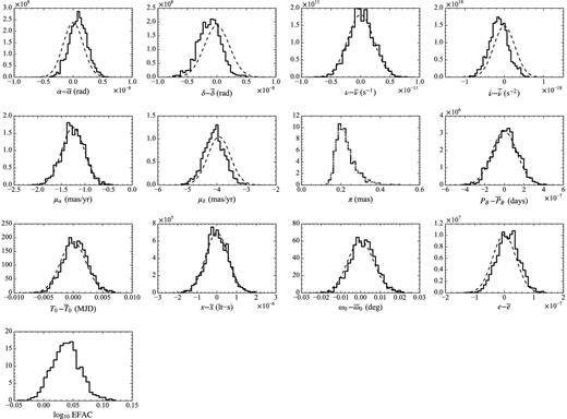
Posterior probability distributions (solid step lines) of the timing parameters for PSR B1953+29. The TOAs were fitted using the DD model. A bar over a parameter refers to the parameter value obtained using tempo2, which are listed in Table 2. The dashed curves show the best-fitting values and errors obtained using tempo2 and the light dotted curve in the parallax plot shows the prior probability distribution, which was derived from the DM distance. The posterior distribution for the parallax is the same as the prior, indicating that the timing observations do not provide any additional information. The posterior distributions for the other parameters agree with the tempo2 timing solution. The tempo2 solution for the parallax is π = −2.7 ± 2.4 mas; we do not plot the corresponding distribution because most of it lies outside of the bayesfit prior and posterior distributions.
Timing solutions for J1640+2224, B1953+29, and J2317+1439 from tempo2.
| Parameter | J1640+2224 | B1953+29 | J2317+1439 |
|---|---|---|---|
| Right ascension, α (J2000.0) | 16:40:16.743 50(6) | 19:55:27.875 96(3) | 23:17:09.237 01(1) |
| Declination, δ (J2000.0) | +22:24:08.9433(7) | +29:08:43.4656(5) | +14:39:31.2449(3) |
| Spin frequency, ν (s−1) | 316.123 984 313 62(3) | 163.047 913 069 140(3) | 290.254 608 187 112(3) |
| Spin frequency derivative, |$\dot{\nu }$| (s−2) | −2.812(1) × 10−16 | −7.907(3) × 10−16 | −2.0475(6) × 10−16 |
| Proper motion, μα (mas yr−1) | 2.2(1) | −1.3(3) | −0.8(2) |
| Proper motion, μδ (mas yr−1) | −11.0(1) | −3.9(4) | 3.1(3) |
| Parallax, π (mas) | −3(2) | −0.7(4) | |
| Orbital period, Pb (d) | 175.460 662 25(7) | 117.349 0971(1) | 2.459 331 4628(3) |
| Orbital period derivative, |$\dot{P_b}$| | 6.4(9) × 10−12 | ||
| Epoch of periastron, T0 (MJD) | 516 26.1796(4) | 461 12.477(3) | |
| Epoch of ascending node, Tasc (MJD) | 540 00.254 766 94(5) | ||
| Projected semimajor axis, x (light-second) | 55.329 7183(7) | 31.412 6902(6) | 2.313 9480(3) |
| Longitude of periastron, ω (deg) | 50.7330(9) | 29.474(7) | |
| Eccentricity, e | 7.9712(3) × 10−4 | 3.3016(4) × 10−4 | |
| ϵ1 ≡ esin ω | 6(2) × 10−7 | ||
| ϵ2 ≡ ecos ω | 1(3) × 10−7 | ||
| |$\dot{\epsilon _1}$| | −2(4) × 10−15 | ||
| |$\dot{\epsilon _2}$| | 2.0(7) × 10−14 | ||
| Orbital inclination, sin i | 0.99a | ||
| Companion mass, m2 (M⊙) | 0.25(4) |
aInclination angle is held fixed at sin i = 0.99.
We conclude that in this case including a prior on the parallax does not change the timing solution. Using bayesfit allows us to validate the linear least-squares solution found with tempo2 and confirms that the parameters’ posterior probability distributions have a Gaussian distribution.
PSR J2317+1439
The observed TOAs for J2317+1439 are fitted using the ELL1 timing model with 15 spin, astrometric, and binary parameters. We also fit the parameter log10EFAC and marginalize posteriors analytically over 42 parameters describing DM variations and pulse-profile variations. The tempo2 timing solution gives a small (and unphysically negative) value of the parallax, π = −0.74 ± 0.38 mas; however, the low DM of 21.9 pc cm−3 implies that this pulsar has a DM distance of only 0.83 kpc and a parallax of 1.2 mas. To explore the timing-model effects of the parallax, we run two variants of our Bayesian analysis: one in which we impose a DM–distance prior on π and another in which we omit π from the timing model (which is equivalent to setting it to zero). For all of the other parameters, we assume a uniform prior centred around the best-fitting value given by tempo2, with width chosen to include the entire posterior.
Fig. 2 compares the bayesfit posterior probability distributions (where the darker solid lines correspond to the DM–distance prior on π and the lighter solid lines to setting π = 0) with the best-fitting normal distributions found with tempo2 (which include π = −0.74 ± 0.38, and are shown as dashed lines). In the prior-on-π analysis, the combination of the prior and of the timing data produces a posterior that favours smaller values of the parallax than the prior. A number of the other parameters are shifted with respect to the tempo2 analysis, particularly the spin frequency and spin frequency derivative. The timing residuals are only slightly different for the two solutions, with an rms of 0.500 μs for the bayesfit posterior-mode solution and 0.496 μs for the tempo2 best-fitting solution. The posterior-mode value of the EFAC parameter is 1.77, which is in good agreement with the reduced χ2 value from the tempo2 analysis (EFAC2 = 3.12, compared with χ2 = 3.03). In the setting-π-to-zero analysis, the timing parameters are again shifted; in fact, their distributions are entirely consistent with a tempo2 run where π is set to zero (not shown here).
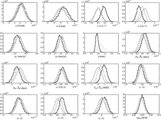
Posterior probability distributions (solid step lines) of the timing parameters for PSR J2317+1439. The TOAs were fitted using the ELL1 model. A bar over a parameter refers to the parameter value obtained using tempo2, which are listed in Table 2. The darker step lines show the posteriors obtained by placing a DM–distance prior (the dotted curve) on π; the lighter step lines show the posteriors obtained by setting π to zero. The dashed curves show the tempo2 normal distributions with π = −0.74 ± 0.38 (which here lies outside the π plot). A tempo2 solution with π set to 0 would lie exactly along the corresponding Bayesian solution. The three timing solutions show significant differences in several parameters.
Thus, we see that either accepting an unphysical best-fitting value for π or excluding it from the timing model leads to a slight but non-negligible bias in a number of other parameters; the bias is corrected in the Bayesian-inference analysis by imposing a physically motivated prior on the parallax. Indeed, in this case, it would be useful to measure the parallax more reliably and accurately using VLBI.
PSR J1640+2224
J1640+2224 deserves special consideration as one of the few systems where it was possible to measure the Shapiro delay (Löhmer et al. 2005). Löhmer and colleagues report a companion mass |$M_2 = 0.15^{+0.08}_{-0.05} \, \mathrm{M}_{\odot }$| and a Shapiro-delay shape sin i ≳ 0.98 (where i is the orbital inclination). Furthermore, Lundgren et al. (1996a,b) identify an optical counterpart to J1640+2224 with properties consistent with a white dwarf of mass ≃ 0.3 M⊙.
The DD timing solution for J1640+2224 adopted by Demorest et al. (2013) fits for 13 parameters describing the spin, astrometric, and binary properties of the system (including M2 but not sin i), and for 49 parameters describing the DM variations and pulse-profile variations with frequency. The parameter sin i cannot be fitted by linear least squares, which would report an unphysical value of i for which the timing model cannot be evaluated, so Demorest and colleagues fix sin i to 0.99, which yields a best fit M2 ≃ 0.3 M⊙. In our analysis, we fit for the 14 spin, astrometric, and binary parameters (including both M2 and sin i) plus the parallax, which is not included in the Demorest et al. (2013) timing solution.
To explore the timing-model effects of incorporating information from optical observations, we run two variants of our Bayesian analysis, one in which we impose physical constraints on i and M2 (with uniform priors cos i ∈ [0, 1] and M2 ∈ [0, 10] M⊙), and another in which we further constrain M2 with a ‘white-dwarf’ prior (a normal distribution centred on 0.3 M⊙ with standard deviation 0.1 M⊙). As in the previous examples, we integrate over the parameters describing the DM variations and pulse-profile shape, and we use a prior distribution for the parallax derived from the DM, which corresponds to a DM distance of 1.16 kpc and a parallax of 0.63 mas. For all of the other parameters, we assume a uniform prior centred around the tempo2 best-fitting values with a sufficiently wide range to encompass the entire posterior.
Fig. 3 compares the posterior probability distributions calculated with bayesfit (the darker solid step lines for the uniform-M2 run and the lighter set for the white-dwarf–prior run) and the tempo2 normal distributions (the dashed curves). The posteriors for the parallax are very close to the prior (the dotted curve). There is significant disagreement between the bayesfit uniform-M2 and the tempo2 timing solutions in the values of the binary parameters, some of which have non-Gaussian distributions. By contrast, the bayesfit white-dwarf–prior distributions are closer to the tempo2 solutions. The residuals however are very similar: for the uniform-M2 solution, the mode of the bayesfit posterior corresponds to residual rms of 0.565 μs compared to the 0.562 μs obtained with the tempo2 solution, and the posterior for EFAC is in good agreement with the best-fitting tempo2 value of reduced χ2 (EFAC2 = 4.47 versus χ2 = 4.35).
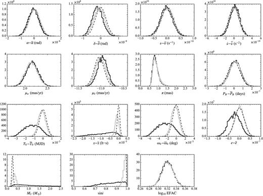
Posterior probability distributions (solid step lines) of the timing parameters for PSR J1640+2224. The TOAs were fitted using the DD model. A bar over a parameter refers to the parameter value obtained using tempo2, which are listed in Table 2. The darker step lines show the posteriors obtained by placing a uniform prior on M2; the lighter step lines show the posteriors obtained by adopting a ‘white-dwarf’ prior for M2 (a normal distribution centred on 0.3 M⊙ with 0.1 M⊙ standard deviation). The dashed curves show the tempo2 normal distributions (and the dashed vertical line shows the fixed tempo2 value for sin i), while the dotted curve traces the DM-distance prior for the parallax. There are significant differences between the three timing solutions in the values of the binary parameters.
In the uniform-M2 solution, the sin i posterior prefers smaller values than reported by Löhmer et al. (2005), corresponding to rather larger companion masses M2. Indeed, the cumulative probability distribution for M2 places only 5 per cent probability below 0.3 M⊙ and 35 per cent probability above the Chandrasekhar limit of 1.44 M⊙, so the timing data alone are not fully compatible with the identification of the counterpart as a low-mass white dwarf. We plot the joint posterior distributions of M2 and sin i in Fig. 4 (where again the darker lines correspond to the uniform-M2 solution, and the lighter lines to the white-dwarf–prior solution). Clearly M2 and sin i are poorly determined and rather correlated, which is not surprising since the measurement of both comes from the Shapiro delay, a weak effect in the timing solution. The white-dwarf–prior distribution is much more constrained, as expected.
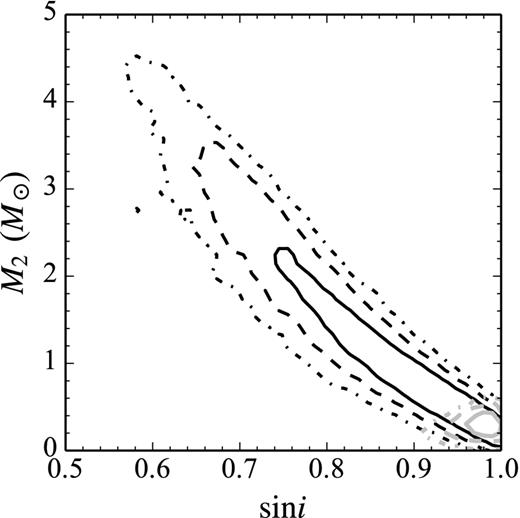
Joint posterior probability distributions of the timing parameters M2 and sin i for PSR J1640+2224. The darker and lighter lines show the posteriors obtained with uniform and ‘white-dwarf’ M2 priors, respectively. The solid, dashed, and dash–dotted lines trace the 68, 95, and 99 per cent confidence intervals, respectively.
This case demonstrates that a non-linear Bayesian analysis can properly characterize timing solutions where a few parameters have weak but non-negligible effects, so both their non-linear behaviour and their acceptable physical ranges come into play, and a linear least-squares approach is insufficient. This case demonstrates also the potential impact of parameter priors from non-timing observations, which are accounted properly in the Bayesian framework. In the light of our reanalysis (especially when we allow for intrinsic pulsar noise, as we do in a forthcoming paper), it would be interesting to revisit the question whether the identification of the J1640+2224 companion is truly definitive.
CONCLUSIONS
In this paper, we have advocated the use of fully non-linear Bayesian inference to derive pulsar-timing solutions, and we have shown that doing so is already practical with current hardware and software. To wit, we have used python wrappers [pymultinest by Johannes Buchner (Buchner 2013) and libstempo by one of us (Vallisneri 2012b)] to connect a powerful stochastic sampler [multinest (Feroz et al. 2009)] with a state-of-the-art pulsar-timing application [tempo2 (Hobbs & Edwards 2006)]. Our code, bayesfit, is available on GitHub for inspection, inspiration, and reuse (Vallisneri & Vigeland 2013).
In Section 2, we have surveyed the mathematical formulation of timing-model fitting and in Section 4, we have shown three practical examples where the non-linear Bayesian analysis provides different benefits: for PSR B1953+29, it validates the linearized least-squares estimates; for PSR J2317+1439, it corrects for parameter-estimation bias by incorporating prior information about the pulsar distance; for PSR J1640+2224, it provides the proper characterization of non-Gaussian posterior parameter distributions, and it accounts for a strong parameter prior from optical observations.
In Section 1, we have suggested two additional applications of Bayesian inference, which may be even more compelling, but which we did not explore practically in this paper.
First, the Bayesian framework is the appropriate formulation for simultaneously inferring the pulsar parameters that have deterministic effects on the timing model and the statistical properties of noise from the pulsar and the detector. Indeed, it is not possible to study noise without simultaneously revisiting the timing model, a point made forcefully by van Haasteren & Levin (2013). Furthermore, unmodelled noise and conceivably GWs will certainly skew the estimates of timing-model uncertainties and even the best-fitting parameters (Lentati et al. 2014).
Secondly, Bayesian-model comparison can provide a quantitative way to choose between alternative timing models, such as one that includes modified-gravity corrections [or even planets (Wolszczan & Frail 1992)] versus one that does not. Such a comparison is most significant when there is a physically well-defined way to attribute prior probabilities to the competing hypotheses, but in the absence of that it is possible to perform a frequentist analysis of a detection scheme (i.e. detection of modified gravity, or planets) based on Bayesian evidence (Vallisneri 2012a).
Lentati et al. (2014) compute the evidence for different noise models and subsets of timing-model parameters, and use its relative values to select a preferred model. The way that they do so raises difficult issues that are typical of Bayesian inference problems for weak signals immersed in noise. For instance, some of the Lentati et al. (2014) noise models include an ‘optimal’ set of lines selected with an iterative procedure. The line-frequency priors should then (but do not) reflect all other sets that could have resulted from the process, and thus penalize the optimal set, a very fine-tuned choice that will perforce fit (or overfit) the data.
Furthermore, the procedure used by Lentati et al. (2014), whereby additional timing parameters are added to the model and retained only if the evidence improves, seems ill-suited to physical parameters such as the first derivatives of the eccentricity and orbital periods. Doing so amounts to comparing models in which some of the physical consequences of general relativity are ‘turned off’. Omitting parameters from a model (which in tempo2 equates to fixing them to zero) should be a question of approximation, not model comparison: it should be done only when it is determined that the corresponding timing-model terms are negligibly small.5 Even if we accepted that such model comparisons are meaningful, they remain ill-defined in the absence of strongly motivated priors for the extra parameters. These priors affect the Occam-factor penalty incurred by the higher dimensional models,6 so they can make the difference between winning or losing a comparison.
We plan to explore these issues in future work.
We are grateful to Paul Demorest, Joe Lazio, Sarah Burke-Spolaor, Rutger van Haasteren, Lindley Lentati, Tom Prince, and to all NANOGrav colleagues for helpful discussions. SV was supported by an appointment to the National Aeronautics and Space Administration (NASA) Postdoctoral Programme at the Jet Propulsion Laboratory administered by Oak Ridge Associated Universities through a contract with NASA. MV was supported by the Jet Propulsion Laboratory RTD Programme. This work was carried out at the Jet Propulsion Laboratory, California Institute of Technology, under contract to the NASA. Copyright 2014 California Institute of Technology.
Although this would be a welcome annoyance, because it would imply rather large GW amplitudes and imminent detections.
The least-squares errors can be construed either as frequentist errors that describe the distribution of the maximum-likelihood estimator across noise realizations or as Bayesian uncertainties that describe the shape of the posterior probability when priors are negligible. Both kinds of errors are reliable only if the model of the data is linear in its parameters, or if its linearization is accurate throughout the region spanned by the predicted errors (Vallisneri 2008). Full Bayesian inference will of course provide exact Bayesian uncertainties; see Vallisneri (2011) for an approach to deriving exact frequentist errors.
Or rather, they rediscovered a well-known result in the theory of Gaussian processes for machine learning (Rasmussen & Williams 2005, section 2.7).
J1713+0747, from Chatterjee et al. (2009).
The same reasoning applies to the phase jumps applied between timings taken at different observatories. These jumps are always present, but could be deemed to be negligible on the basis of experimental considerations.
This is unless the extra parameters are determined so poorly that they populate the priors uniformly, in which case the evidence is unchanged.
