


Abstract
We present a simple toy model to understand what sets the scatter in star formation and metallicity of galaxies at fixed mass. According to this model, the scatter ultimately arises from the intrinsic scatter in the accretion rate, but may be substantially reduced depending on the time-scale on which the accretion varies compared to the time-scale on which the galaxy loses gas mass. This model naturally produces an anticorrelation between star formation and metallicity at a fixed mass, the basis of the fundamental metallicity relation. We show that observational constraints on the scatter in galaxy scaling relations can be translated into constraints on the galaxy-to-galaxy variation in the mass loading factor at fixed mass, and the time-scales and magnitude of a stochastic component of accretion on to star-forming galaxies. We find a remarkably small scatter in the mass loading factor, ≲ 0.1 dex, and that the scatter in accretion rates is smaller than that expected from N-body simulations.
1 INTRODUCTION
Large galaxy surveys in the past decade have taught us that star-forming galaxies fall on a main sequence (MS), a tight correlation between their stellar mass and star formation rates (SFRs; Daddi et al. 2007; Elbaz et al. 2007; Noeske et al. 2007). This correlation contains remarkably little scatter – the SFR varies by about ±0.34 dex at fixed stellar mass (Whitaker et al. 2012; Guo, Zheng & Fu 2013).
The existence of the star-forming MS and its small scatter has substantially affected our understanding of galaxy evolution. The cosmological paradigm of the past few decades, Λ cold dark matter, predicts that dark matter haloes, and hence the galaxies occupying them, form hierarchically – large haloes are built from mergers of smaller haloes. The expectation was therefore that mergers between galaxies would be a major driver of their evolution over cosmological times, frequently triggering starbursts. The small scatter in the MS at multiple redshifts has shown, however, that most galaxies are not in fact experiencing any dramatic effects of major mergers (Rodighiero et al. 2011), and most stars form in ‘normal’ galaxies lying along this relation.
In addition to the MS, galaxies follow other scaling relations. Practically, this means that at a given point in cosmic history many properties of galaxies are set by a single parameter associated with the galaxy's mass. This fact has led to the development of a series of models dubbed ‘equilibrium’, ‘regulator’, or ‘bathtub’ models (Dekel, Sari & Ceverino 2009; Bouché et al. 2010; Cacciato, Dekel & Genel 2012; Davé, Finlator & Oppenheimer 2012; Genel, Dekel & Cacciato 2012; Feldmann 2013; Lilly et al. 2013), in which the properties of a galaxy are self-regulated near a stable equilibrium between accretion of gas, star formation, and outflows. The fundamental ingredients are an SFR that increases with increasing gas mass in the galaxy, and a time-scale on which the gas reservoir returns to its equilibrium value much shorter than the time-scale on which bulk properties of the galaxy (mass, accretion rate, outflow efficiency, star formation time-scale, etc.) vary.
Equilibrium models have enjoyed success in heuristically reproducing the average trends in galaxy evolution. However, such models are inherently incapable of quantifying higher order effects, including scatter in individual scaling relations and various fundamental metallicity relations (FMRs), found by numerous groups (Mannucci et al. 2010; Mannucci, Salvaterra & Campisi 2011; Yates, Kauffmann & Guo 2012; Bothwell et al. 2013; Lara-López, López-Sánchez & Hopkins 2013; Stott et al. 2013; Dekel & Mandelker 2014), typically parametrized as a quadratic function Z(M*,SFR).
Many theoretical studies are focused on reproducing first-order relations, which is sufficiently difficult in and of itself that second-order relations are often neglected (however, for an exception, see Dutton, Bosch & Dekel 2010). In principle, however, to fully understand galaxy evolution we should be able to understand not only average or median galaxy properties, but their full distribution. A significant advantage of the equilibrium models is that fitting them to any first-order relation is trivial, so extending them to understand the higher order relations is easier than with any other method.
In this work, we take one step beyond equilibrium models, allowing the mass accretion rate to vary with a fixed lognormal scatter. Such a scatter is expected based on N-body simulations (e.g. Neistein & Dekel 2008) and hydrodynamic simulations (e.g. Dekel et al. 2013). Depending on the time-scale on which the accretion rate varies, a population of these galaxies may never be in equilibrium. That is, their masses and metallicities may change substantially. However, they may still reach a statistical equilibrium, in which the full joint distribution of all galaxy properties becomes time invariant.
In Section 2, we introduce the basic formulation of this model and explore the implications for the origin of the width of the star-forming MS. We add metallicity to the model in Section 3, allowing us to examine the FMR and the scatter in the mass–metallicity relation (MZR, the correlation between stellar mass and gas-phase metallicity). The model we construct in these sections is independent of the first-order effects considered by most equilibrium models, which allows us to avoid uncertainty in the numerical values of numerous important parameters in galaxy evolution (e.g. the mass loading factor). In Section 4, we re-dimensionalize our model, taking a guess at the correct scalings and normalizations to use, and demonstrate the ability of this model to understand unknown physics based solely on the scatter in galaxy scaling relations. We discuss the limitations of our model, quantitative constraints it can place on the accretion process, and alternative explanations for the intrinsic width of these relations in Section 5, and conclude in Section 6.
2 A MINIMAL MODEL FOR SCATTER IN THE MS
This equation has exactly the same structure as the radiative transfer equation where accretion acts as the source term, time in units of mass-loss time-scales is similar to the optical depth, and the instantaneous value of Ψ is analogous to the intensity of radiation.
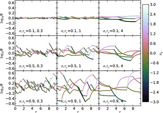
Ψ as a function of time. Recall that Ψ is the dimensionless mass-loss rate, which at fixed mass we take to be proportional to both gas mass and SFR. For each pair of σ (the intrinsic scatter, increasing top to bottom) and τc (the ratio of the coherence time to the mass-loss time, increasing left to right), we show the trajectories of five random galaxies over the course of a randomly selected 10 star formation times and coloured by the instantaneous value of x(t) – lighter colours mean higher accretion rates. The galaxies exponentially approach |$\Psi = {\rm e}^{\sigma x_k}$|, so when τc is large, the scatter in Ψ reflects the intrinsic scatter σ, but when τc is short, the many changes in the accretion rate never allow the galaxies’ mass-loss rates, Ψ, to reach the accretion rate |${\rm e}^{\sigma x_k}$| – instead they remain near the average value.
In the limit that τc ≫ 1, only the most recent draw from the distribution matters and all previous draws are exponentially suppressed. In the opposite limit, τc ≪ 1, the leading factor |$1-{\rm e}^{-\tau _{\rm c}} \rightarrow \tau _{\rm c} \approx N_\mathrm{loss}^{-1}$|, where Nloss is the number of draws from the accretion rate distribution in a given mass-loss time. For very short coherence times, Ψk becomes an average of the lognormal accretion rates over the most recent mass-loss time-scale, with more recent accretion rates weighted somewhat more heavily. The full probability distributions of Ψ and Ψk (which serves as an approximation to Ψ) for various values of τc and σ are shown in Fig. 2, along with the probability distributions of the five most recent draws from the appropriate lognormal distributions which are added together to give Ψk. As the coherence times grow longer (panels from left to right), fewer draws from the accretion rate contribute to the current mass-loss rate. As the intrinsic scatter in the accretion rate increases (top to bottom), the probability densities of the draws from the accretion rate overlap more, meaning that it is increasingly likely that the most recent accretion rate is not the largest contributor to the current mass-loss rate.
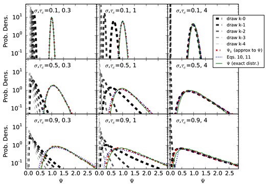
The construction of the distribution of Ψ, the dimensionless mass-loss rate. The red, blue, and green lines show the probability density of a galaxy with a given combination of σ and τc having, at a randomly selected time, a given value of Ψ. Green shows the full distribution, red shows the distribution of Ψk, namely Ψ at a switch in the accretion rate, and blue shows the analytic approximation to Ψk. These approximations are remarkably good, at least for this selection of σ and τc. The dashed grey lines show the lognormal distributions from which numbers are drawn and added together to compute Ψk. As τc increases, fewer draws from the accretion distribution contribute to Ψ, until eventually only the last draw matters and all the others are exponentially suppressed (rightmost panel). As the intrinsic width of the accretion distribution increases (top to bottom), the accretion rate distributions increasingly overlap, increasing the chances that the most recent accretion rate does not dominate in determining the current value of Ψ.
In the limit of short τc, the fraction |$(1-{\rm e}^{-\tau _{\rm c}})/(1+{\rm e}^{-\tau _{\rm c}})$| reduces to τc/2. Thus, when σ is also sufficiently small (namely σ2 ≪ 1), the variance of Ψk reduces to σ2τc/2. Physically, when the accretion rate varies rapidly compared to the mass-loss time, any individual draw from the accretion rate distribution becomes unimportant and all that matters is the long-term average. The exception is when σ is large, in which case extremely large accretion rates become common and |$\sigma _{\Psi _k}$| again approaches σ, though we caution that the distribution becomes less lognormal as σ increases with small τc. Fig. 3 shows |$\sigma _{\Psi _k}$| computed with a Monte Carlo simulation (for details see Appendix A).
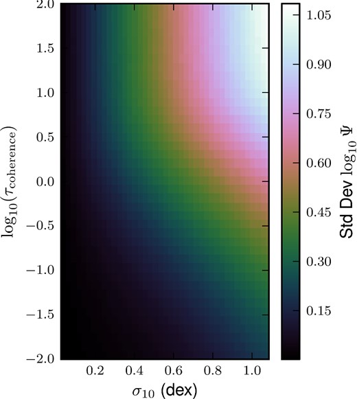
The width of the ‘MS’. Each pixel represents an ensemble of galaxies with fixed τc and σ, wherein the mass-loss rate Ψ was measured for each galaxy at a random time. The standard deviation of log10Ψ in each bin is plotted above. Longer coherence times (upwards in the plot) allow the galaxies to equilibrate so that Ψ approaches the accretion rate, so the scatter in Ψ approaches σ. More precisely, the standard deviation of log10Ψ approaches σ10 = σ/ln (10), the standard deviation of |$\log _{10} \dot{M}_\mathrm{ext}$|. Coherence times shorter than the mass-loss time-scale, i.e. log 10τc ≲ 1, lead to a reduction in the scatter roughly in proportion to τc – individual draws from the accretion rate matter increasingly less, and the galaxies do not have enough time for Ψ to approach the accretion rate before it changes.
From this discussion, we see that τc and σ compete in setting the width of the MS – recall that |$\Psi \propto \dot{M}_\mathrm{SF}$| at fixed mass, so the logarithmic scatter in Ψ is the logarithmic scatter in the MS, modulo some complications that will be addressed in Section 5. Even after |$\sigma _{\Psi _k}$| has been scaled by the intrinsic accretion rate, both σ and τc enter the expression for the MS scatter. This suggests that σ may be interpreted as a third time-scale in the problem, namely the number of mass-loss times necessary to forget a typical accretion event.
3 INCLUDING METALLICITY
The SFR, taking into account galactic winds and stellar evolution (see equation 2), is |$\dot{M}_\mathrm{SF} =(f_{\rm R}+\eta )^{-1} M_{\rm g}/t_\mathrm{loss}$|. The yield y is defined as the mass of metals produced during the course of stellar evolution per unit mass of gas locked in stellar remnants – if 1000 M⊙ of gas forms stars, a total of yfR1000 M⊙ of metals will be produced by these stars and returned to the interstellar medium (ISM). For the galactic wind metallicity, the usual assumption throughout the literature on chemical evolution is that Zw = Z, i.e. before gas is ejected from a galaxy by stellar feedback, it is assumed to be perfectly well mixed with the ambient ISM (for recent exceptions, see Recchi et al. 2008; Peeples & Shankar 2011; Krumholz & Dekel 2012; Vogelsberger et al. 2013). This is a strong assumption because galactic winds are likely to be preferentially metal enriched. Physically, this is because metals are produced in the same places, sometimes by the same events, which are likely to cause galactic-scale outflows, namely sites of recent star formation, where massive stars emit ionizing radiation and end their lives as supernovae.
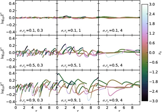
Z† as a function of time. For each pair of σ (the intrinsic scatter in the accretion rate, increasing top to bottom) and τc (the ratio of the coherence time to the mass-loss time, increasing left to right), we show the trajectories of five random galaxies over the course of a randomly selected 10 star formation times and coloured by the instantaneous value of x(t) – lighter colours mean higher accretion rates. We can immediately see that high accretion rates tend to lead to low metallicities. We also see that for large coherence times (rightwards), each galaxy reaches an extremum in metallicity before returning to its equilibrium value (Z† = 1). Short coherence times mean that the accretion rate changes when the galaxy is near this extremum or before, meaning the ensemble width of log10Z† will tend to peak near τc ∼ 1, and the relationship between metallicity and SFR will be strongest (most anticorrelated) for τc ≲ 1.
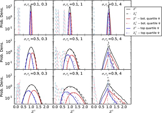
The construction of the distribution of the normalized metallicity, Z†. For the same parameters shown in the previous figures, we plot the PDF of Z† (solid line), the approximation to it using |$Z^\dagger _k$| (equation 23), and we also split the probability distribution into galaxies with high (low) SFRs in blue (red). We can immediately see that high-metallicity galaxies tend to have low SFRs, though the probabilities do overlap substantially. Light blue and red lines show the PDF of the contributions to |$Z^\dagger _k$|, split into the top and bottom quartiles in SFR, from old terms in the summation of equation (23). As with Ψ, the probability distribution of Z† may be thought of as the sum of a series of random draws wherein the influence of older draws is exponentially forgotten, although galaxies which end up in the blue (red) bin at the present time are likely to have had preferentially higher (lower) SFRs in the past, at least for τc ≲ 1. Unlike with Ψ, Z† becomes noticeably non-lognormal for larger values of τc, since galaxies sampled at a random time are likely to be near the equilibrium value Z† = 1, regardless of the accretion rate.
We can also see that in this regime the distribution of Z† is not lognormal. We can none the less compute the standard deviation of log Z†, shown in Fig. 6, for different fixed values of σ and τc. This has an observational counterpart in the scatter in the MZR, so we will use these predictions as a guide to understand how the observed scatter can constrain this model. The contours in Fig. 6 are substantially different from those in Fig. 3, so the scatter in the MS and the MZR may provide complementary constraints on the model. The physical reason is that for τc ≳ 1, galaxies’ metallicities are less and less affected by the intrinsic scatter σ for increasing τc, whereas for increasing τc the scatter in the SFR approaches the intrinsic scatter. The metallicities are unaffected because regardless of σ, Z → Zeq over a few mass-loss times.
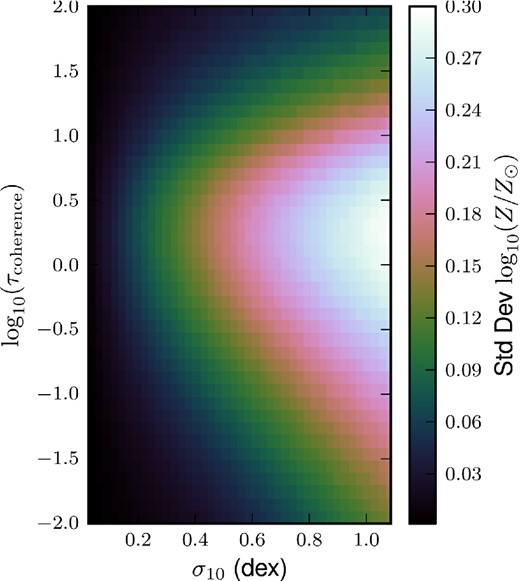
The width of the MZR. Each pixel represents an ensemble of galaxies with fixed τc and σ10 = σ/ln (10), wherein the metallicity Z was measured for each galaxy at a random time. The standard deviation of log 10Z/Z⊙ in each bin is plotted above. Longer coherence times (upwards in the plot) allow the galaxies to equilibrate so that Z approaches Zeq (a constant value regardless of the accretion rate). Coherence times shorter than the mass-loss time-scale, i.e. log 10τc ≲ 0, lead to a reduction in the scatter roughly in proportion to τc – individual draws from the accretion rate matter increasingly less. Larger intrinsic scatters (rightwards in the plot) negate this effect by making large accretion events typical.
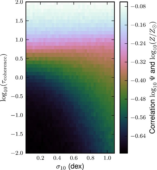
The correlation between Ψ and Z/Z⊙. For small scatters and rapid variability in the accretion rate, the SFR and metallicity are substantially anticorrelated. Increasing the coherence time allows galaxies to return to their equilibrium Z regardless of the accretion rate, wiping out the anticorrelation.
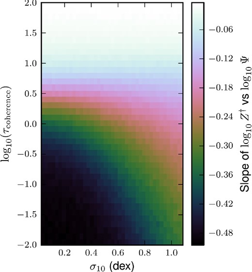
The ‘slope of the FMR’. For each τc and σ10 = σ/ln (10), we fit a linear model to the scatter plot of log10Ψ versus log 10(Z/Z⊙) of all galaxies drawn from the distribution, and plot the resulting slope here. We find uniformly that the slope is negative, though the slope flattens for large values of τc, and to a lesser degree, for large values of σ because the metallicity in each case becomes less sensitive to the current value of the accretion rate. Either it is approaching its fixed equilibrium value (large τc) or it is being more heavily influenced by past very dramatic accretion events (large σ10).
4 CONSTRUCTION OF GALAXY SCALING RELATIONS – AN INITIAL GUESS
The results we have derived thus far, namely the joint probability density of Ψ and Z†, are applicable only at fixed values of μ, σ, tcoherence, tloss, ZIGM, and q. We refer to an ensemble of galaxies with fixed values of these parameters as a simple (or stationary) galactic population (SGP). As we saw in the previous sections, the only variables which affect the joint distribution of Ψ and Z† are σ and |$\tau _{\rm c} = t_\mathrm{coherence}/t_\mathrm{loss}$|. However, to compute physical quantities, i.e. the SFR, the metallicity, etc., one must specify the other variables.
The power of our approach using SGPs is that, to a reasonable approximation, the properties of a star-forming galaxy are set by a single parameter having to do with the size of the galaxy (e.g., stellar mass, halo mass, or K-band luminosity). One could therefore hope that, at a fixed stellar mass, the population of galaxies may be well described by a single SGP. Essentially, all of the scalings of mass loading factor, accretion rate, etc. which account for the slope and zero-points of galaxy scaling relations would be taken out, leaving only the intrinsic scatter.
Here we make an educated guess as to how to map the dimensionless model presented in the first few sections of this paper to observable galaxy scaling relations. Although alternative assumptions may be preferred by other practitioners, we hope that this exercise will be at least illustrative. In Section 4.1, we use results from N-body-only dark matter simulations to make guesses for the parameters of the accretion process: μ, σ, and tcoherence. Each of these parameters thereby has a predicted scaling with halo mass and redshift. In this procedure, we leave one free parameter fϵ, a constant less than unity, to describe how much the accretion rate is reduced below this guess. We then adopt the assumptions that y = 0.054, fR = 0.54 [appropriate for a Chabrier (2005) initial mass function (IMF) with yields from solar-metallicity stars Maeder (1992) – see appendix A of Krumholz & Dekel (2012)], ZIGM ≪ 0.02, and ξ = 0. To fully specify the SGP model, the only remaining parameters are η, tdep, and fϵ. In Section 4.2, we adopt a value of fϵ and power-law scalings of tdep and η with halo mass such that we fit three galaxy scaling relations: M* versus SFR, Z, and Mg/M*. To do so, we need to assign a value of M* to each halo mass, for which we take the Behroozi, Wechsler & Conroy (2013a,b) relations with a fixed lognormal scatter of 0.19, consistent with various observational constraints (Behroozi et al. 2013b; Reddick et al. 2013).
With all of these parameters specified as a function of halo mass and redshift, we can construct synthetic versions of these galaxy scaling relations, including their intrinsic scatter, and the higher order FMR, Z(M*, SFR). Section 4.3 describes how we take the synthetic relations and extract three higher order quantities which we will use to constrain our model: the scatter in the MS, the scatter in the MZR, and the ‘slope’ of the FMR, namely the logarithmic derivative of the metallicity with respect to the SFR at fixed stellar mass. These three quantities can then be compared directly to observations, which allows us to rule out our initial guess, and non-trivially constrain σ, tcoherence, and other potential sources of scatter (Section 5.1). The parameters used throughout the paper are summarized in Table 1.
Important parameters used in this study.
| Parameter | Equations | Description |
|---|---|---|
| The accretion process | ||
| μ | 3, 28 | The log base e of the median baryonic accretion rate |
| σ | 3, 28 | The lognormal scatter in the (DM and baryonic) and accretion rate |
| Δω | 30 | The scale-free time step taken to generate accretion histories |
| tcoherence | 3, 30 | The time over which the accretion rate is constant before a new random value is drawn |
| ϵ | 28, 29 | The fraction of |$f_{\rm b} \dot{M}_{\rm DM}$| which reaches the gas reservoir |
| fϵ | 29 | A fixed fraction by which the baryonic accretion rate may be reduced – fixed by first-order scaling relations |
| ZIGM | 12 | Metallicity of infalling baryons, fixed at 2 × 10⁻⁴ |
| Star formation | ||
| |$\dot{M}_\mathrm{SF}$| | 2 | The star formation rate |
| Mg | 1, 2 | The gas mass available to form stars |
| η | 2 | The ratio of mass lost in galactic winds to stars formed – fixed by first-order scaling relations |
| tdep | 2 | The depletion time, |$M_{\rm g}/\dot{M}_\mathrm{SF}$| – fixed by first-order scaling relations |
| fR | 2 | The remnant fraction – fraction of mass not returned to the ISM from a simple stellar population, fixed at 0.54 |
| tloss | 1, 2 | The loss time, i.e. the time-scale on which the reservoir is depleted, tdep/(η + fR) |
| y | 12 | Mass of metals returned to the ISM per mass locked in stellar remnants, fixed at 0.054 |
| ξ | 13 | Metallicity enhancement of galactic winds, fixed at 0 (perfect mixing) |
| q | 15 | A combination of y, fR, ξ, and η we call the effective yield |
| SGP parameters | ||
| τc | 5 | tcoherence/tloss – an input to the SGP |
| σ10 | 3, 28 | This is the same σ as above, but divided by ln 10 – an input to the SGP |
| Ψ | 4, 5 | The ratio of the mass-loss rate (Mg/tloss) to the median accretion rate eμ – an output of the SGP |
| Z† | 18, 19 | The metallicity of the gas reservoir, subtracting out ZIGM and normalizing to q – an output of the SGP |
| xk | 3 | For a given galaxy, the kth draw from a standard Gaussian, which sets the accretion rate |
| Other sources of scatter (see especially Section 5.1) | ||
| |$\sigma _{\log _{10} M_*}$| | – | Lognormal scatter added to M*(Mh), assumed uncorrelated with anything else |
| |$\sigma _{\log _{10} t_{\rm dep}}$| | – | Lognormal scatter added to the depletion time |
| |$\sigma _{\log _{10} \eta }$| | – | Lognormal scatter added to the mass loading factor η |
| σμ | – | Gaussian scatter in μ. This is like including a stochastic component whose coherence time ≫tloss |
4.1 Baryonic accretion
4.2 Fitting the first-order relations
To compute τc and re-dimensionalize the SGP, we still need to know the mass-loss time-scale, i.e. the depletion time and η, as well as ξ. These values are sufficiently uncertain that it is worth digressing to discuss how they may be chosen to fit the first-order galaxy scaling relations, namely the star-forming MS, the MZR, and the stellar mass–gas mass relation.
To compare our model with many galaxy scaling relations, computed as a function of stellar mass M*, we must pick an M*. Since our model is purely equilibrium based, we have no way to compute integrated quantities like M* besides appealing to other empirical relations. We employ the Behroozi et al. (2013a,b) model of the relation between stellar mass and halo mass, including a scatter in stellar mass at a fixed halo mass of 0.19 dex (Reddick et al. 2013). Another common approach is to simply use M* rather than Mh (Lilly et al. 2013) as the parameter by which to scale the SGP parameters (η, ξ, etc.).
Given these equilibrium relations, we attempt to find power-law scalings of η and tdep, and a constant value of fϵ, which will roughly fit the observed galaxy scaling relations. This leads us to take fϵ = 0.5, η = (Mh/1012 M⊙)− 2/3, and tdep = 3 Gyr (Mh/1012 M⊙)− 1/2, as described below. These fits were done by hand, which is reasonable given the uncertainties in the mean relations.
For the mean relations themselves, we take the summaries of this data from Peeples & Shankar (2011) – these are plotted as the coloured lines and the points with error bars in Fig. 9. The data themselves largely come from the Sloan Digital Sky Survey (SDSS), with the exception of the gas masses. The fits use stellar masses from Tremonti et al. (2004) and Kauffmann et al. (2003), and SFRs from Brinchmann et al. (2004), both of which include aperture corrections. Metallicities are estimated by Kewley & Ellison (2008) using a variety of strong line metal calibrations from the literature, and then corrected by Peeples & Shankar (2011) to use a Chabrier (2003) IMF. The gas fraction data come from McGaugh (2005), Leroy et al. (2008), and Garcia-Appadoo et al. (2009).
![Scaling relations. We compare observed galaxy scaling relations and their scatters (coloured lines) with scaling relations (black lines) calculated by drawing galaxies (coloured points) from a sequence of SGPs using reasonable guesses of how the SGP parameters scale with halo mass. The left-hand panel is our initial guess, while the right-hand panel shows an improved guess which better fits the observational constraints on the scatter in these relations. In particular, the initial guess yields a model MS with intrinsic width wider than the observed scatter, while the improved guess has a much small intrinsic scatter. The colours indicate offset from the MS, namely the black dashed line fitted in the top panel. PS11 refers to Peeples & Shankar (2011), and T+04 and PP04 refer to metallicity calibrations used by Tremonti et al. (2004), and the [N ii]/Hα calibration from Pettini & Pagel (2004).](https://oup.silverchair-cdn.com/oup/backfile/Content_public/Journal/mnras/443/1/10.1093/mnras/stu1142/2/m_stu1142fig9.jpeg?Expires=1716592590&Signature=lR0JuoBnpJcQp2sUj07AIM6zGKX6Q4w3SxYq4UV6G0YPR0QUmTkqgt6Xr-joVyJgTUDpWv-GHKhOS3kwkWCrf7Oq-IV9rZzxAN65dFILMr6B14SCC35ezLusadDGyOM6bGG0Dtca4UevZF4CofWSdsAGxxIfdrqAwSLGpJLlOQ9f-4Rb8tLM5DEFhnd7CmIaKZebvScVYZ7DWJ9TelMqLPL4xYJt0sEGzcAxqZ3l-rSZEwF2ZJz5ehay8G0VSBYL~zYk2yPaYWuis-WVr9OKZGGyT0MIAP9lISbFB4MfuAoSXAVSvZQAPigh~6GOw1heZyjCOV0hFpxG7ydswq8pWQ__&Key-Pair-Id=APKAIE5G5CRDK6RD3PGA)
Scaling relations. We compare observed galaxy scaling relations and their scatters (coloured lines) with scaling relations (black lines) calculated by drawing galaxies (coloured points) from a sequence of SGPs using reasonable guesses of how the SGP parameters scale with halo mass. The left-hand panel is our initial guess, while the right-hand panel shows an improved guess which better fits the observational constraints on the scatter in these relations. In particular, the initial guess yields a model MS with intrinsic width wider than the observed scatter, while the improved guess has a much small intrinsic scatter. The colours indicate offset from the MS, namely the black dashed line fitted in the top panel. PS11 refers to Peeples & Shankar (2011), and T+04 and PP04 refer to metallicity calibrations used by Tremonti et al. (2004), and the [N ii]/Hα calibration from Pettini & Pagel (2004).
To approximately fit the centres of the observed z = 0 MS, we had to use a steep scaling of the mass loading factor with halo mass, namely η = (Mh/1012 M⊙)− 2/3. This is a result of the short cooling times and/or cold streams in low-mass haloes which efficiently supply cold gas at a rate proportional to the dark matter accretion rate, which is much larger than the observed SFR in these galaxies. That is, ϵ is large for low-mass galaxies in our initial guess. If low-mass galaxies are in statistical equilibrium, these large values of η are necessary. It is possible that some other physical process is decreasing ϵ at these masses, or that the galaxies are not in equilibrium (Krumholz & Dekel 2012; Kuhlen et al. 2012; Kuhlen, Madau & Krumholz 2013). In the latter scenario, η may vary quite weakly, leaving the mass-loss time-scales at low masses to be comparable to the depletion times, themselves comparable to or much longer than the age of the Universe. We discuss this possibility further in Section 5.2, but for now we adopt |$\eta \propto M_{\rm h}^{-2/3}$|.
We do not fit the MZR particularly well in this simple model (see Fig. 9). That is, most calibrations of the MZR are not well described by the power law in Mh we assume here. This is not extremely concerning given the systematic uncertainties in the observations. The scaling of η needed to fit the star-forming MS does leave the MZR in the right neighbourhood, without adjusting the fiducial values of ZIGM = 2 × 10⁻⁴ ≈ Z⊙/100, ξ = 0, or fϵ and η.
In contrast, the gas fraction data are fitted remarkably well by our fiducial scalings. Given the reasonable fit of the SFR–M* relation, we were left with one parameter to vary to fit Mg/M*-M*, namely tdep. Despite the (lack of) trends from the GASS (Schiminovich et al. 2010) and COLD GASS (Saintonge et al. 2011) surveys in the total gas depletion time with mass, we find that we need tdep = 3 Gyr (Mh/1012 M⊙)− 1/2. Since η scales even more steeply, the mass-loss time-scale actually shortens with decreasing halo mass in this scenario, scaling as |$t_\mathrm{loss} \propto M_{\rm h}^{1/6}$|.
The two reference models we use to generate synthetic galaxy scaling relations and FMRs.
| Initial guessa | Improved guessb | |
|---|---|---|
| σ10 (dex) | 0.45 | 0.225 |
| Δω | 0.5 | 0.2 |
| |$\sigma _{\log _{10} M_*}$| (dex) | 0.19 | 0.07 |
| |$\sigma _{\log _{10} t_{\rm dep}}$| (dex) | 0 | 0 |
| |$\sigma _{\log _{10} \eta }$| (dex) | 0 | 0 |
| σμ (dex) | 0 | 0.08 |
| Initial guessa | Improved guessb | |
|---|---|---|
| σ10 (dex) | 0.45 | 0.225 |
| Δω | 0.5 | 0.2 |
| |$\sigma _{\log _{10} M_*}$| (dex) | 0.19 | 0.07 |
| |$\sigma _{\log _{10} t_{\rm dep}}$| (dex) | 0 | 0 |
| |$\sigma _{\log _{10} \eta }$| (dex) | 0 | 0 |
| σμ (dex) | 0 | 0.08 |
aBased on N-body simulations.
bAdjusted to fit both the conservative observational constraints and the much tighter |$-2 < \mathrm{\partial} \log Z/\mathrm{\partial} \log \dot{M}_\mathrm{SF} < -1$|.
The result of applying these scalings is shown in Fig. 9. For each Mh below 1012.3 M⊙ provided in the Behroozi et al. (2013a,b) M*(Mh) relation, we apply the scalings above to compute the necessary physical parameters to specify the SGP, draw 300 samples from the SGP, and assign each one a stellar mass according to M*(Mh), plus a fixed scatter, |$\sigma _{\log _{10} M_*} = 0.19$| dex. The resultant population of galaxies, as designed, fits various observational constraints at z = 0, represented in each figure by the various coloured lines (which include representative scatters) from Peeples & Shankar (2011). The black lines show power-law fits and the computed ±1σ scatter of the population. The observational fits are not necessarily precise, and in particular the MZR famously has many different fits depending on which calibration is used (Kewley & Ellison 2008). The two columns in Fig. 9 have the same scalings of tdep, η, and q, but different values of σ, Δω, and |$\sigma _{\log _{10} M_*}$|. The left column shows the initial guess discussed here and in the previous section, while the right column has values of the accretion process parameters more in line with observations (the ‘improved guess’ model – see Table 2 and Sections 4.3 and 5.1). We have chosen the range of M* to extend somewhat below the minimum stellar masses used in the various summaries of the SDSS data from Peeples & Shankar (2011), up to the stellar mass associated with the quenching of star-forming galaxies and hence their departure from the star-forming MS (Cheung et al. 2012).
It is worth emphasizing that fitting or not fitting the observed relations should be construed neither as success nor failure for our model – the equilibrium relations (equations 31, 32, and 33) have enough free parameters that fitting the observations is not challenging. However, it is encouraging that relatively little tuning was required for reasonable fits, and that we end up with models with a reasonable physical basis: energy-driven winds for |$\eta \propto M_{\rm h}^{-2/3}$| (see Murray, Quataert & Thompson 2005 for the basics of energy- versus momentum-driven winds), long depletion times at low masses owing to low H2 fractions, η of order unity, and tdep of the order of 3 Gyr at high masses.
4.3 Information in the scatter
Now that we have a reasonable fit for the redshift zero–median relations, we can return to our main goal – understanding the higher order relationships in the data. In particular, we would like to understand the scatter in the MS and the MZR, and the (negative) slope implied by the FMR of metallicity with respect to SFR at fixed stellar mass. Now that we have synthetic data, we can follow a simple procedure to fit a synthetic MS, MZR, and FMR. For the former two, we simply fit a linear model with least-squares regression to (the log base 10) of SFR versus M* and Z versus M*. For each synthetic galaxy, we can then subtract off the linear fit for SFR or Z at that galaxy's M* to find its residual. Finally, the scatter is calculated as the sample standard deviation of the residuals.
For all three of these quantities – the two scatters and the (logarithmic) slope of Z versus |$\dot{M}_\mathrm{SF}$| at fixed stellar mass – we can compare both to observations and to predictions from the full joint distribution of Ψ and Z† by a single SGP (Figs 3, 6, and 8). The scatters in the MS, MZR, and FMR are not identical to that in an SGP because the relationship between stellar and halo mass also has some scatter. Thus, a population of galaxies at fixed M* represents a weighted sum of SGPs.
Thus, there will be additional scatter in these synthetic observations, as compared to the SGP predictions. This is illustrated in Fig. 10 – we compare the input values of τc and σ10 (the coloured points, nearly on top of each other) to the values of τc and σ10 the SGP model would predict given the values of the synthetic scatters. That is, we construct a synthetic scaling relation, measure its scatter, and then plot the appropriate contour from Fig. 3, 6, or 8. When we artificially set |$\sigma _{\log _{10} M_*} = 0$|, these contours converge at the input values, but including the scatter in M* flattens the FMR slope and increases the scatter in the MS and MZR, leaving a general region in τc–σ10 space where the contours are close to each other, but no trivial way to recover the input values.
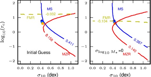
Information in the scatter of the MS and MZR. The coloured points near (0.45, 0.8) represent the values of τc and σ10 in the ‘initial guess’ model as a function of a wide range of halo masses. With a random realization of the initial guess model, we extract the scatter in the MS and MZR (quoted in fig. 9), and the linear slope |$\mathrm{\partial} \log Z/\mathrm{\partial} \log \dot{M}_{\rm SF}$| of the FMR. We can then find the contours in Figs 3, 6, and 12 corresponding to these values, i.e. the set of σ10 and τc the SGP would predict if we provide it with these two scatters and the FMR slope. These contours are shown as the coloured lines – the numbers for each contour are the scatters in the MS and MZR (blue, red), and the slope in the FMR (yellow) which we feed to the contour maps. When we do not include any uncorrelated scatter in the stellar mass (right-hand panel), the lines intersect at the input value, but including a reasonable scatter in M* (left-hand panel) increases the scatters in the MS and MZR and flattens the FMR slope.
This at once shows both the promise and the difficulty of using observed second-order relations to predict these parameters. The constraints are largely independent of each other, so one could hope to non-trivially constrain the acceptable values of σ10 and τc. However, additional sources of scatter not included in the simple dimensionless SGP predictions can make it difficult to recover the values of these parameters simply by reading off where the contours intersect in this diagram.
None the less, this diagram (Fig. 10) and the associated SGP predictions (Figs 3, 6, and 8) provide some heuristic guidance. We see that in this parameter space, the input values of σ10 and τc are nearly independent of halo mass. This means that the fiducial model would predict no change in the scatters of the MS or MZR, nor any change in the slope of the FMR, which is roughly consistent with observations (Whitaker et al. 2012; Zahid et al. 2013). We also see that to reduce the synthetic scatter to below the observed scatter, ≲ ±0.34 dex for the MS and ≲ ± 0.1 dex (Kewley & Ellison 2008, both of which may be regarded as upper limits on the intrinsic scatters), we could reduce the input accretion scatter, σ, or dramatically reduce the coherence time (and therefore τc). Our ‘improved guess’ model adjusts the initial guess to reduce the two scatters and steepen the FMR slope. In particular, we reduce σ by a factor of 2 and Δω in our estimate of tcoherence to 0.25 (see the next section).
5 DISCUSSION
In the previous section, we set up a fiducial set of assumptions to map the SGPs of Sections 2 and 3 into observable parameters. We were easily able to match the first-order relations, but our first guess produced scatters in our synthetic MS and MZR that were too large. In this section, we examine in more detail the full range of SGP-based models that are consistent with the observed constraints on the scatters in the MS and MZR and the slope of the FMR, and the range of halo masses and redshifts over which SGP-based models are valid in principle.
5.1 A more general model – do all galaxies at a fixed Mh correspond to one SGP?
The analysis of SGPs in Sections 2 and 3 explicitly assumes that a given galaxy has had the same values of μ, σ, tloss, tcoherence, ZIGM, and q for eternity. This is clearly false – galaxies increase their mass over time, moving them along any presumed scaling relations in e.g. tdep or η, while other quantities likely depend explicitly on time, e.g. μ and tcoherence. The statistical equilibrium model we have proposed here, and other simpler models, may still be successful in describing galaxies because these quantities plausibly vary slowly relative to the internal time-scales of the galaxy, i.e. the loss time. Whereas the typical equilibrium model assumes this of the accretion rate, our model relaxes that particular assumption and allows the accretion rate to vary, possibly very quickly, relative to other time-scales.
Our model was constructed with the goal of understanding the scatter in galaxy scaling relations by examining the role of a known (and significant) scatter in dark matter accretion rates among galaxies at a given mass. However, it is also plausible that the mass loading factor, the depletion time, or some other quantity may vary between galaxies near a fixed mass, or within a given galaxy on relatively short time-scales. The former situation may be handled by our model by having multiple SGPs with different values of e.g. η at the same mass. The latter situation cannot be handled by SGPs as we have formulated them.
The scenario in which scatter in η, tdep, or μ is responsible for the scatter in galaxy scaling relations has several distinct predictions compared to the stochastic accretion model we have presented. In particular, the scatter, rather than being stochastic, would be constructed from several nearly parallel, slightly offset, equilibrium relations. One could likely find acceptable values for the scatter in the SGP parameters which reproduced the observed scatters, since each equilibrium relation depends on a different combination of the SGP parameters. Thus, one might expect to be able to have eμ vary by ∼0.34 dex and ZIGM to vary by ∼0.1 dex.
This model would indeed produce, more or less, the observed scatters in the MS and MZR, but it would not account for the decreasing metallicity with increasing SFR at fixed stellar mass (see Fig. 11), i.e. what we call the ‘slope’ of the FMR. In particular, the equilibrium metallicity is independent of the accretion rate, and the SFR is independent of ZIGM (at least in this simple model), so there would be no slope in the FMR. The situation gets even worse with a scatter in η, since both the equilibrium SFR and Z are inversely related to η, which would tend to create a positive slope in the FMR. Similarly, a scatter in M* at fixed halo mass tends to induce a positive slope – at a given M*, galaxies from higher halo mass and lower halo mass will be present, and because both the MS and MZR have positive slopes, the higher (lower) halo mass galaxies will have higher (lower) SFRs and Zs, again leading to a positive slope in the FMR.
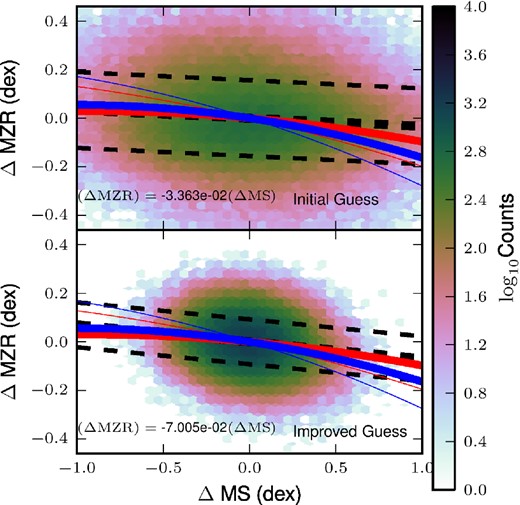
Displacements from first-order scaling relations. Here we show the offset of galaxies, in both our initial guess and improved guess models, from fits to their MS and MZR. The black lines show a linear fit to these data points, and the 1σ scatter of galaxies in Δ MZR around this fit. The coloured lines show predictions of these quantities from two different fits to the z = 0 FMR using different metallicity calibrations, with the thin lines corresponding to M* = 108 M⊙ and the thick to 1011 M⊙. Here we can see the slight, but significant observed and predicted anticorrelation between SFR and metallicity. Note that to fill out this histogram we drew a sample of 100 times the number of galaxies shown in Fig. 9.
Given the difficulty in obtaining a negative FMR by adding scatters in the parameters which enter the equilibrium relations, compared with the natural way the negative slope arises in our statistical equilibrium model, via a time-varying accretion rate, it certainly seems that no alternative model is needed. In fact, by enforcing the requirement that |$\mathrm{\partial} \log Z/\mathrm{\partial} \log \dot{M}_\mathrm{SF} <0$|, we may be able to obtain limits on the scatter in parameters (M*, η) which tend to make the slope in the FMR positive. We caution, however, that the uncertainty in the metallicity determinations is great enough that for some methods of computing the metallicity, the slope becomes positive at high masses (Yates et al. 2012). For now we keep the weak, but perhaps not weak enough, restriction that |$\mathrm{\partial} \log Z/\mathrm{\partial} \log \dot{M}_\mathrm{SF}<0$| and see what constraints we can derive.
To accomplish this, we set up a six-dimensional grid of models. Each point in the grid corresponds to a choice of σ10, log10Δω, scatter in M*, scatter in tdep, scatter in η, and scatter in eμ. For each point in the grid, we simulate a full set of galaxies – 200 per value of Mh < 1012.3 M⊙, and compute the scatter in the MS and MZR and the slope in Z versus SFR at fixed M*. We then compare each of these pieces of information to the observations in a maximally conservative way. We treat the observed scatters in the MS and MZR as upper limits on the intrinsic scatters, and make no assumptions about the purely observational scatter. Although there is an observationally known value of the slope of Z versus SFR at fixed M*, we make no strong assumptions about the probability distribution function (PDF) of that parameter – we merely require that it is negative (see Fig. 12). Thus, for each point in the grid, we can say how many constraints that model violates: 0, 1, 2, or 3.
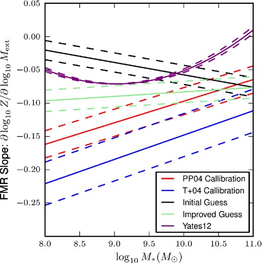
Slope in the FMR. For both our improved and initial guesses, as well as three fits to the z = 0 FMR using different metallicity calibrations, we show the slope in the metallicity with respect to the SFR, as a function of stellar mass. Since the FMR fits depend explicitly on |$\dot{M}_\mathrm{SF}^2$|, we must also choose an SFR at which to evaluate this quantity. We choose the MS value at that mass (as determined by our fit to the MS of our initial guess model), which we plot as the solid lines, and ±0.3 dex, the dashed lines. The three different calibrations predict substantially different values, so to be somewhat conservative we have chosen to interpret the observational constraint as |$\mathrm{\partial} \log Z/\mathrm{\partial} \log \dot{M}_\mathrm{SF} < 0$|, a fact on which most calibrations agree most of the time.
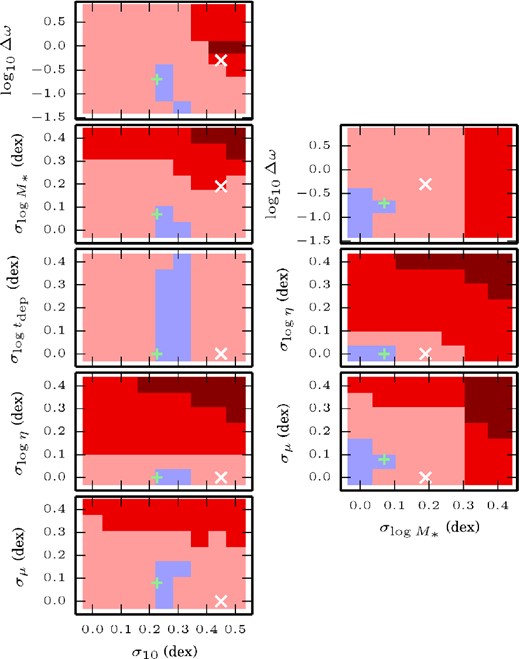
In Fig. 13, we project these scores, again in a maximally conservative way. For each point in the 2D projection, we look up all models in the full 6D space which have the two values under consideration in our projection, and we find the model which violated the fewest constraints. Thus, the figure shows the minimum number of constraints violated by any model with that combination of values. If any model with those coordinates is allowed by the constraints, the pixel is shown in blue. Each darker shade of red means every model with those coordinates violated at least one more constraint, up to all three.
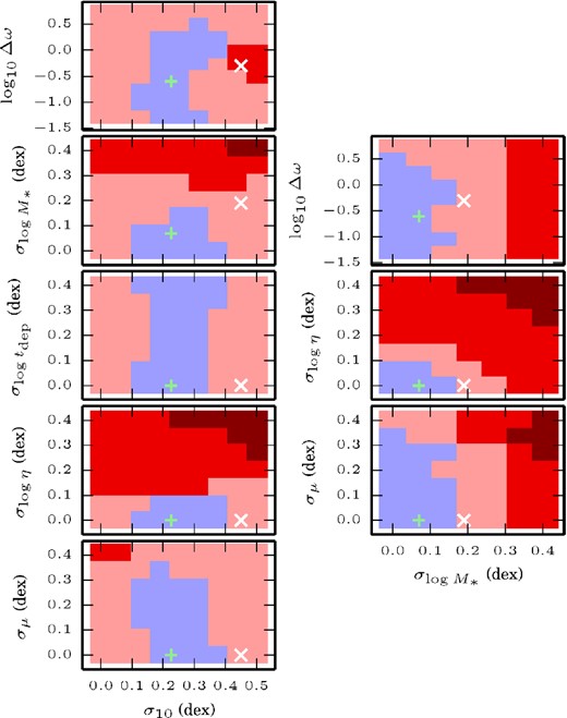
The set of parameters conservatively allowed by the observations. In addition to the parameters of the accretion process (σ10 and Δω), we include a variable lognormal scatter in η, M*, tdep, and the median accretion rate eμ. These lognormal scatters have medians equal to the values used in Section 4.2 to fit the first-order relations. Blue pixels indicate that at least one model with that pair of parameters is consistent with the data. Each darker shade of red means the model which violates the fewest constraints for that pair of parameters violates one more constraint, up to all three. The white cross shows our initial guess, while the green ‘+’ shows our ‘improved guess’.
This exercise demonstrates that even this conservative interpretation of the observed scatters as upper limits, combined with the weak requirement that Z decrease with increasing SFR at fixed stellar mass, yields non-trivial constraints on the parameters. In particular, σ10 ≲ 0.35 dex, smaller than that in our fiducial model. This may point to a smoothing out of the baryonic accretion rate relative to the scatter in dark matter accretion rates implied by the Neistein et al. (2010) formula. Perhaps even more interesting is that there is a minimum σ10 implied by our observational restrictions, σ10 ≳ 0.1 dex, which comes from the requirement that the FMR have a negative slope. In particular, if σ10 is too small, the subtle feature in the M*(Mh) relation causes both the SFR and metallicity of galaxies with M* ∼ 109 M⊙ to be higher than the MS and MZR, and galaxies at other masses to be below those relations, generating a positive correlation between SFR and Z. However, other versions of the M*–Mh relation do not necessarily included this feature.
The scatter in M* for a given SGP must be ≲ 0.1 dex. This is a bit at odds with the observational constraints from Reddick et al. (2013) (0.20 ± 0.03 dex at fixed maximum circular velocity), although we note that our constraint is on scatter in M* that is uncorrelated with everything else in the SGP, whereas in reality it is quite plausible (and in fact predicted by the SGP – see Appendix A) that, at a fixed halo mass, M* is correlated with both SFR and Z. This number can also be comparable to the 0.09 dex uncertainty in stellar mass reported by Tremonti et al. (2004), though again our constraint is only on the scatter in M* that is uncorrelated with all other observables.
Another interesting constraint is that the scatter in η must be ≲ 0.1 dex. This is surprisingly small, considering the great deal of theoretical uncertainty as to the actual values and scalings of η in the first place. In our models, this comes from the aforementioned effect that in the equilibrium relations, both Z and |$\dot{M}_\mathrm{SF}$| are inversely related to η, so scatter in η tends to reverse the negative slope in the FMR.
Unsurprisingly, there is virtually no constraint on the scatter in tdep. This is simply because the equilibrium relations for |$\dot{M}_\mathrm{SF}$| and Z are independent of tdep – to constrain this scatter one would need constraints on the scatter in the M*–Mg/M* relation, although if such galaxies also had SFR measurements, they would have directly measured depletion times anyway. There is also relatively little constraint on scatter in the median accretion rate, eμ. Essentially this is because, in the equilibrium relations, only the SFR is affected by this scatter, so as long as the scatter in eμ is smaller than the scatter in the MS, there is no problem.
With these constraints in mind, we have altered our initial guess, simply by reducing σ10, Δω, and |$\sigma _{\log _{10}M_*}$|, and slightly increasing σμ (see Table 2). We label this model the ‘improved guess’ model. Purely for demonstration, we have also computed scores for the grid of models where we include not only an upper limit on the scatters, but also a much narrower range of acceptable slopes of the FMR, namely |$-2 < \mathrm{\partial} \log Z/\mathrm{\partial} \log \dot{M}_\mathrm{SF} < -1$|. With these stronger restrictions, we get the projections shown in Fig. 14. Our ‘improved guess’ model is engineered to adhere to this much stronger constraint, though there are plenty of models which would be ruled out by this strict scoring that are still consistent with the observations. Unsurprisingly, the stronger constraint dramatically narrows the range of acceptable models in most of the projections. Particularly striking is that the allowed range of Δω ∼ Δz, the interval in redshift over which galaxies have constant accretion rates in our model, is narrowed substantially from Δω ≲ 3 to Δω ≲ 0.4.
A plausible set of constraints on model parameters. Here we make the plausible but uncertain assumption that the FMR slope, |$\mathrm{\partial} \log Z/\mathrm{\partial} \log \dot{M}_\mathrm{SF}$|, is between −2 and −1, in addition to the constraints on the widths of the MS and MZR. As one might expect, narrowing the allowed range of FMR slopes dramatically reduces the allowed regions of parameter space. One should not take these regions to be genuine constraints, but rather to demonstrate the power of the slope of the FMR in constraining these parameters.
5.2 Domain of applicability
Under what circumstances might a real population of galaxies be in statistical equilibrium? We know that for a constant accretion rate, the SFR and the metallicity will equilibrate on the mass-loss time-scale. A standard equilibrium model therefore requires that tloss be much less than the time-scale on which any parameter entering into the equilibrium relations, namely q (i.e. η, ξ, and fR), ZIGM, tdep, and |$\dot{M}_\mathrm{ext}$|, changes. The success of these models in understanding the first-order trends in galaxy scaling relations suggests that these requirements, while seemingly numerous, are at least marginally satisfied.
Our statistical equilibrium model relaxes one of these restrictions by splitting |$\dot{M}_\mathrm{ext}$| into a (hopefully) slowly evolving median eμ and a (potentially) rapidly varying stochastic component eσx(t). Our formulation of this component introduces two time-scales, tcoherence – the time between new draws from the lognormal distribution, and σtloss – the time for a 1σ accretion event to be forgotten by the galaxy.
Figs 2 and 5 show graphically the exponential suppression of old draws of the accretion distribution in their influence on the full distribution of Ψ and Z†. In logarithmic space, the separation between the centres of the distribution of each draw is just |$\tau _{\rm c} = t_\mathrm{coherence}/t_{\rm loss}$|, while the width of each distribution is σ. When σ ≲ τc, the distributions are well separated, and we conclude that galaxies may be in statistical equilibrium so long as tloss is appreciably less than the time-scale on which any parameters of the SGP change (explicitly μ, σ, tcoherence, tloss, ZIGM, and q). Note that tcoherence itself may well be shorter than or comparable to tloss.
When σ ≳ τc, the contributions from previous draws begin to matter significantly for the distribution of Ψ. In this case, the number of draws which are important increases from ∼1 to ∼ σ/τc, so rather than tloss being short, we need σtloss to be short. At least in our initial guess, shown in the previous section, this is a minor effect since σ ∼ 1. Therefore, the region of Mh–z space where the statistical equilibrium model is valid should be comparable to the region where an ordinary equilibrium model is capable of reproducing the first-order galactic scaling relations, which in turn is set by the scaling of tloss with halo mass and redshift.
In our fiducial model presented in the previous section, star-forming galaxies at every halo mass were in equilibrium at z = 0. As we mentioned, this is not necessarily the case in the real Universe – the mass loading factor may well scale weakly with halo mass, in which case low-mass galaxies, with their long depletion times, would be unable to equilibrate to their baryonic accretion rate even in a Hubble time. Either scenario is currently perfectly consistent with observations, since the mass-loss time-scale is unknown, owing to its dependence on η. In Fig. 15, we show regions of Mh–z space where the equilibrium assumptions are valid – the bluer the colour, the better satisfied the condition that the Hubble time be much longer than teq, the maximum of the mass-loss time (tloss), the coherence time (tcoherence), and the burn-through time (σtloss).
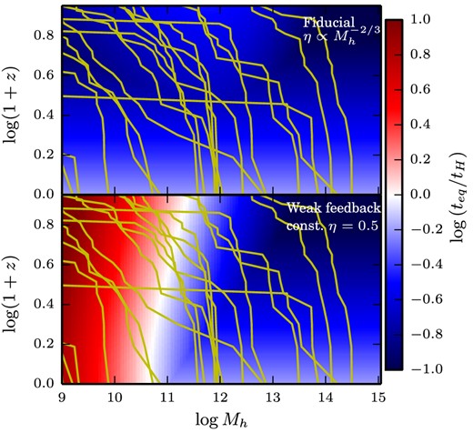
The validity of the statistical equilibrium model. Here we show the ratio of teq to the instantaneous Hubble time, as a function of halo mass and redshift. The bluer the colour, the more satisfied the condition that teq < tH, required for the statistical equilibrium model to be valid. We show two cases for the scaling of the mass loading factor with halo mass: |$\eta \propto M_{\rm h}^{-2/3}$|, which we use in our fiducial model, and η = 0.5. Both are consistent with direct observations of η. For reference, we overplot the trajectories of 20 haloes as they grow stochastically, as calculated by equations (25)–(27) with Δω = 0.5. With a strong scaling for η in halo mass and tdep in redshift, the model is reasonable for haloes probed in galaxy surveys, but it is certainly plausible that low-mass galaxies are not in equilibrium.
To construct these diagrams, we also need to make an assumption regarding how input parameters vary not only with halo mass, but with redshift. We assume that the mass loading factor and the factor by which we reduce the efficiency, fϵ, are independent of redshift, but that the depletion time-scales as tdep ∝ (1 + z)−1, a somewhat weaker scaling than if the depletion time scaled with the dynamical time (Davé et al. 2012). This scaling is consistent with recent observational results from CO observations at high redshift (Tacconi et al. 2010, 2013; Saintonge et al. 2013), though of course there are large uncertainties. Moreover, these observations span a very limited range of mass and redshift compared to that shown in these diagrams. We therefore emphasize that these plots represent plausible assumptions, not predictions.
5.3 Evolution with redshift
Since it is plausible that a statistical equilibrium model may be used successfully at higher redshift, one may consider extending our analysis beyond the z ≈ 0.1 data we have considered. There are however both theoretical and observational challenges. First, a great deal of poorly justified assumptions are required to scale the fiducial model to higher redshift, including the strong scaling of depletion time with redshift discussed in the previous section. Observationally, while there are measurements of the MS, MZR, and FMR at higher redshift, the metallicity measurements in particular are fraught with complications arising from the changing set of lines visible from ground-based telescopes and the uncertainty of converting line characteristics to physical metallicities in the substantially different environments of high-redshift galaxies (see Kewley et al. 2013a,b). The high-order quantities we discuss in this paper are therefore both difficult to predict and measure.
We can none the less make the basic point under the assumption that the SFR and metallicity have reached their equilibrium values, the metallicity will be Zeq = ZIGM + q, where q is a combination of fR, η, and ξ, none of which are expected to change dramatically with redshift. Thus, the MZR should not change with redshift if galaxies are in equilibrium. Observational studies tend to find at least some evolution (e.g. Mannucci et al. 2009; Yuan, Kewley & Richard 2013). However, given the difficulty in calibrating the zero-point of the MZR even at low redshift, and the possibility that samples of high-redshift galaxies are biased high in SFR and therefore low in Z (Stott et al. 2013), we do not believe that equilibrium models have been ruled out at higher redshifts.
We can also describe how the fiducial model, which does not quite fit the data at z = 0, would scale to higher redshift. The predicted value of σ is not dependent on redshift, at least for the dark matter. Given our results suggesting that baryonic processes likely play an important role in smoothing the accretion, it is unclear how this smoothing process would evolve, so this constant value of σ is highly uncertain. Meanwhile tcoherence will evolve strongly with redshift, but the quantity which sets the second-order scatter we consider is |$\tau _{\rm c} = t_\mathrm{coherence}/t_\mathrm{loss}$|. If we assume that η at fixed halo mass does not change, then tloss simply scales as the depletion time, which likely does decrease significantly towards higher redshift. If they decrease at a similar rate, near 1/(1 + z), then τc is unlikely to evolve very much. In this scenario, we would predict that the scatter in the MS and MZR, and the slope in the FMR at fixed stellar mass would be roughly independent of redshift (and as evidenced in Fig. 10, independent of halo mass).
5.4 Relationship to other work
Our model bears a resemblance to several recent papers on equilibrium models (Davé et al. 2012; Lilly et al. 2013). Our model reduces to a slightly simpler version of the Davé et al. (2012) model when τc → ∞ and σ → 0, i.e. the upper left of the σ10-τc diagrams we showed in Sections 2 and 3.
One of the criticisms of the Davé et al. (2012) model has been its explicit assumption that dMg/dt = 0. Simple toy models of the growth of galaxies under various star formation laws, (e.g. Feldmann 2013), point out that for many galaxies at redshift zero, dMg/dt < 0. Indeed, in our recent work on the radially resolved evolution of disc galaxies since z = 2 (Forbes et al. 2014), we find that much of the galactic disc for many galaxies tends to be moderately out of equilibrium between local sources and sinks, with star formation being somewhat higher than the (local) accretion rate.
The equilibrium model of Lilly et al. (2013) attempts to address this issue by allowing part of the incoming accretion to build up in the gas reservoir. The price they pay is that the SFR becomes an input to their model rather than an output. Perhaps even more worrying is that they assume dZ/dt = 0 always, even when |$\mathrm{d} M_{\rm g}/\mathrm{d}t \ne 0$|. Note that Feldmann (2013) makes a similar argument. As shown by our sample trajectories in Section 3, it actually takes Z longer to equilibrate than the SFR, since the metallicity can only equilibrate once the SFR catches up (or falls off) to the accretion rate. It is therefore odd that they assume that the metallicity is in equilibrium while the SFR is not. It is only through this oddity that they are able to fit a second-order relation, i.e. the FMR, with their model. We consider our model to be both more self-consistent and more powerful, in that we can generate a scatter in the SFR and metallicity, and about the FMR itself. Pipino, Lilly & Carollo (2014) have recently examined the validity of the equilibrium approximations made in these models and the resulting relationship between specific SFR and metallicity, and find reasonable agreement between their numerical model and Lilly et al. (2013)'s approximation.
Another important result, and to our knowledge the only previous theoretical attempt to address the scatter in the MS, is Dutton et al. (2010). They use a rather sophisticated semi-analytic model, including cooling from virial shock-heated gas in a dark matter halo and star formation as a function of specific angular momentum (i.e. radius) in the disc, although they do not include any way for the gas to change its angular momentum (as we do in Forbes, Krumholz & Burkert 2012; Forbes et al. 2014). They find a significant but small scatter in their model star-forming MS arising from variation in halo concentration, which in turn causes differences in the mass accretion histories between different galaxies of the same halo mass. Their model therefore resembles ours in the limit that τc → ∞, but σ ≠ 0. Our model's more flexible treatment of the accretion process and other model parameters (e.g. the mass loading factor) gives us somewhat more insight on the problem of scatter not only in the MS but also in the MZR and FMR, although of course our model is far simpler in terms of its treatment of star formation, and we can make no predictions regarding other important and interesting quantities (Dutton 2012, i.e. galaxy sizes and rotation curves).
6 CONCLUSION
In the past few years, a new view has emerged as a useful way of understanding galaxies. In this picture, galaxies are in a slowly evolving equilibrium between accretion, star formation, and galactic winds regulated by the mass of cold gas in their ISM. To the degree that the parameters controlling this balance are well-defined functions of the mass of a galaxy and its redshift, this sort of model may be used to understand the connection between galaxy scaling relations and these physical parameters, which are not known from first principles.
In the spirit of these equilibrium models, we have presented a simple model which relaxes a key assumption in the equilibrium model, namely that the rate at which baryons enter the gas reservoir varies slowly. A population of galaxies in our model has been fed by the same stochastic accretion process for eternity, or at least long enough that the full joint distribution of all galaxy properties has become time invariant. We therefore refer to our picture as a statistical equilibrium model, since the individual galaxies are not in equilibrium, but the population is.
With this model, we study a number of second-order relationships about the well-known galaxy scaling relations between the stellar mass and the SFR (the star-forming MS), and the stellar mass and metallicity (the MZR). We look at the scatter at fixed stellar mass in both of these quantities, as well as the (anti)correlation between star formation and metallicity at fixed stellar mass. Our main conclusions are as follows.
Including a stochastic scatter in the accretion rate at the level expected from N-body cosmological simulations naturally produces an anticorrelation between SFRs and metallicities at fixed stellar mass, as observed, and a scatter in both the star-forming MS and MZR somewhat larger than the observed scatters.
Neglecting the scatter in model parameters (i.e. the mass loading factor, the depletion time, the scatter in stellar mass at fixed halo mass, etc.), all second-order quantities (the scatter in the MS, the scatter in the MZR, and the slope in metallicity with respect to the SFR at fixed stellar mass) are determined by only two parameters: the scatter in the accretion rate and the ratio of the time-scale on which the accretion varies to the time-scale on which the galaxy loses gas mass.
Using a maximally conservative interpretation of the available data, we are able to constrain these two parameters as well as a number of additional parameters, namely the scatter in the mass loading factor at fixed halo mass and the uncorrelated scatter in M* at fixed halo mass. We find that the lognormal scatter in the baryonic accretion rate σ10 is between about 0.1 and 0.4 dex, moderately smaller than what we would have predicted based on N-body simulations and assuming that the baryons follow the dark matter. This may point to some process in the haloes of galaxies which smoothes out variations in the baryonic accretion rate, or a substantial amount of baryon cycling, which has the effect of averaging out the accretion rate over a longer time period. We find that the scatter in the mass loading factor at fixed halo mass is less than 0.1 dex, remarkably small considering the theoretical uncertainty in the details of the physics of feedback. Our constraint on the time-scale over which the accretion rate varies is much weaker, with the allowed time period exceeding a change in redshift of 1, but it could be narrowed considerably by stronger constraints on the FMR.
The statistical equilibrium framework we have presented here is a novel approach to understanding higher order properties of galaxy scaling relations analytically. This sort of analysis may be plausibly extended to other galaxy properties beyond what we have considered here, or to other astrophysical applications involving a self-regulated process being driven stochastically. For our particular application of this method, we hope that our analysis motivates new development in both theory and observation.
On the theory side, tcoherence (or a more sophisticated quantity describing the time-scales on which accretion varies) and σ may be measured with some confidence in both dark-matter-only and baryonic cosmological simulations. Semi-analytic models may be altered to include the appropriate level of variability in baryonic accretion rates. Meanwhile, we have shown that observable quantities, e.g., the scatter in the star-forming MS, can provide significant constraints on properties of the baryonic accretion process and the galaxy-to-galaxy variability of the mass loading factor. Our inferences are, however, limited by our limited certainty on the intrinsic scatter in the scaling relations we have considered and the true parameters of the FMR. Pinning down these quantities observationally at a variety of masses and redshifts may substantially improve our understanding of the details of baryonic accretion and feedback.
JCF is supported by the National Science Foundation Graduate Research Fellowship under Grant Nos DGE0809125 and DGE1339067. MRK acknowledges support from the NSF through CAREER grant AST-0955300 and by NASA through ATFP grant NNX13AB84G. AB acknowledges support from the Cluster of Excellence ‘Origin and Structure of the Universe’. AD was supported by ISF grant 24/12, by GIF grant G-1052-104.7/2009, by a DIP grant, and by the I-CORE programme of the PBC and the ISF grant 1829/12. The Monte Carlo simulations detailed in Appendix A were carried out on the UCSC supercomputer Hyades, which is supported by NSF grant AST-1229745. We would like to thank Erica Nelson, Pieter van Dokkum, Peter Behroozi, and Eyal Neistein for helpful conversations, and the anonymous referee for a helpful report.
Max Planck Fellow.
Note that the quadratic fits reported in the literature are typically fits to 12 + log 10(O/H), whereas here we are fitting to the metallicity. This only makes a difference in the a0 term, and not to the slope with respect to the SFR at fixed stellar mass, on which we will concentrate.
REFERENCES
APPENDIX A: DETAILS OF THE MONTE CARLO SIMULATIONS
Throughout this paper, we have presented heatmaps of various quantities as a function of |$\tau _{\rm c} = t_\mathrm{coherence}/t_\mathrm{loss}$|, and σ10 = σlog 10(e). Computing each of these quantities for the model is typically a non-trivial task which requires a Monte Carlo simulation, in which a large ensemble of galaxies are sampled at random times to sample the underlying true distribution of the quantity in question for galaxies in this model. Here we describe the details of these simulations.
For each pixel in these grids of τc versus σ10, we sample an ensemble of 30 000 galaxies. Each galaxy is started at a time τ = 0 with initial values Ψ = Z† = 1, the equilibrium values for those quantities in the limit σ → 0 and τc → ∞. The galaxies are then evolved for long enough that, for all practical purposes, they forget their initial conditions (formally our model assumes that the galaxy population has been undergoing the same stochastic accretion process for eternity, but this is obviously impractical computationally). To determine ‘long enough’, we use the analytic results derived in Sections 2 and 3 which show that galaxies forget their initial conditions with an e-folding time of tloss. We also note that for our distribution to represent the true long-term steady-state distribution, as discussed in Section 5.2, galaxies with large scatters in their accretion rate need to experience enough draws from the accretion rate distribution that even the tail of the probability distribution of past events has no influence on the present distribution.
We therefore define a time-scale |$\tau _\mathrm{long} = 1 + \tau _{\rm c} + \sigma$|, i.e. a time guaranteed to be of the order of the longest time-scale in the problem for any choice of τc and σ. We then calculate the number of draws from the accretion distribution necessary to simulate each galaxy out to 15τlong, namely |$k = 15 \tau _\mathrm{long} / \tau _{\rm c}$|. We then draw a pseudo-random number uniformly distributed between 0 and 1, and compute the galaxy's properties (Ψ, Z†) at the time |$\tau _\mathrm{obs} = (k+r) \tau _{\rm c}$|, where r is the random number. This samples the full distribution of these quantities for the population of galaxies in steady state. In general, the computational cost is just proportional to k, since to compute Ψ and Z†, we must first draw k random numbers and compute the sequence Ψ1, …, Ψk and |$Z^\dagger _1,\ldots ,Z^\dagger _k$| before we can calculate those quantities at τobs. Thus, the models with short coherence times, i.e. τc ≪ 1, are the most expensive.
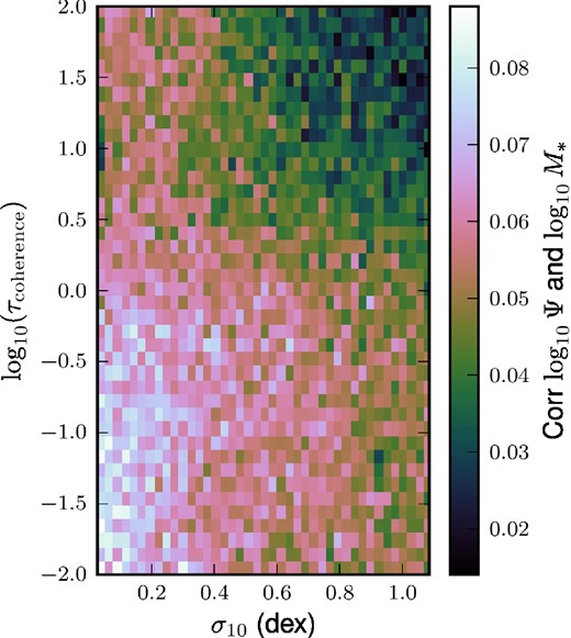
The correlation between SGP versions of the SFR and stellar mass. The non-zero correlation shows that scatter in stellar mass at fixed halo mass can drive galaxies along the MS, rather than being merely uncorrelated.
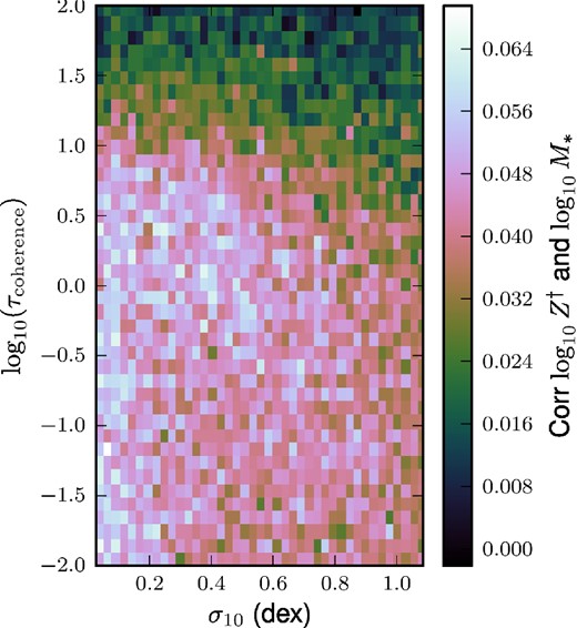
The correlation between SGP versions of the metallicity and the stellar mass. Just as with the SFR, the correlation is positive everywhere, meaning again that scatter in stellar mass at fixed halo mass scatters galaxies along the MZR.
