


Abstract
We develop a novel abundance matching method to construct a mock catalogue of luminous red galaxies (LRGs) in the Sloan Digital Sky Survey (SDSS), using catalogues of haloes and subhaloes in N-body simulations for a Λ-dominated cold dark matter model. Motivated by observations suggesting that LRGs are passively evolving, massive early-type galaxies with a typical age ≳5 Gyr, we assume that simulated haloes at z = 2 (z2-halo) are progenitors for LRG-host subhaloes observed today, and we label the most tightly bound particles in each progenitor z2-halo as LRG ‘stars’. We then identify the subhaloes containing these stars to z = 0.3 (SDSS redshift) in descending order of the masses of z2-haloes until the comoving number density of the matched subhaloes becomes comparable to the measured number density of SDSS LRGs, |$\bar{n}_{\rm LRG}=10^{-4} \,h^3\, {\rm Mpc}^{-3}$|. Once the above prescription is determined, our only free parameter is the number density of haloes identified at z = 2 and this parameter is fixed to match the observed number density at z = 0.3. By tracing subsequent merging and assembly histories of each progenitor z2-halo, we can directly compute, from the mock catalogue, the distributions of central and satellite LRGs and their internal motions in each host halo at z = 0.3. While the SDSS LRGs are galaxies selected by the magnitude and colour cuts from the SDSS images and are not necessarily a stellar-mass-selected sample, our mock catalogue reproduces a host of SDSS measurements: the halo occupation distribution for central and satellite LRGs, the projected autocorrelation function of LRGs, the cross-correlation of LRGs with shapes of background galaxies (LRG–galaxy weak lensing) and the non-linear redshift-space distortion effect, the Finger-of-God effect, in the angle-averaged redshift-space power spectrum. The mock catalogue generated based on our method can be used for removing or calibrating systematic errors in the cosmological interpretation of LRG clustering measurements as well as for understanding the nature of LRGs such as their formation and assembly histories.
1 INTRODUCTION
Galaxy redshift surveys are one of the primary tools for studying the large-scale structure in the Universe (Davis & Huchra 1982; de Lapparent, Geller & Huchra 1986; Kirshner et al. 1987; York et al. 2000; Peacock et al. 2001). Over the coming decade, astronomers will have even larger surveys including Baryon Oscillation Spectroscopic Survey1 (BOSS; Dawson et al. 2013), WiggleZ2 (Blake et al. 2011), VIMOS Public Extragalactic Redshift Survey (VIPERS),3 Fibre Multi Object Spectrograph (FMOS),4 Hobby-Eberly Telescope Dark Energy Experiment (HETDEX),5 BigBOSS6 (Schlegel et al. 2009), Subaru Prime Focus Spectrograph (PFS;7 Ellis et al. 2012), Euclid8 and Wide Field Infrared Survey Telescope (WFIRST).9 The upcoming generation of galaxy redshift surveys is aimed at understanding cosmic acceleration as well as measuring the composition of the Universe via measurements of both the geometry and the dynamics of structure formation (Eisenstein, Hu & Tegmark 1999; Wang, Spergel & Strauss 1999; Tegmark et al. 2004; Cole et al. 2005).
On large scales, galaxies trace the underlying distribution of dark matter, and their clustering correlation is a standard tool to extract cosmological information from the measurement. Because of their relatively high spatial densities and their intrinsic bright luminosities, luminous red galaxies (LRGs) are one of the most useful tracers (Eisenstein et al. 2001; Wake et al. 2006). Measurements of the clustering properties of LRGs have been used to measure the baryon acoustic oscillation (BAO) scale (Eisenstein et al. 2005; Percival et al. 2007; Anderson et al. 2012) as well as to constrain cosmological parameters (Tegmark et al. 2004; Cole et al. 2005; Reid et al. 2010; Saito, Takada & Taruya 2011).
Our lack of a detailed understanding of the relationship between galaxies and their host haloes complicates the analysis of large-scale clustering data. The halo occupation distribution (HOD) approach or the halo model approach has provided a useful, albeit empirical, approach to relating galaxies to dark matter (see e.g. Peacock & Smith 2000; Seljak 2000; Scoccimarro et al. 2001, for the pioneer works). In these approaches, the distribution of haloes is first modelled for a given cosmological model, e.g. by using N-body simulations, and then galaxies of interest are populated into dark matter haloes. The previous works have shown that, by adjusting the model parameters, the HOD-based model well reproduces the autocorrelation functions of LRGs measured from the Sloan Digital Sky Survey10 (SDSS; Zehavi et al. 2005; Zheng, Coil & Zehavi 2007; Wake et al. 2008; Reid & Spergel 2009; White et al. 2011). It has been shown that LRGs reside in massive haloes with a typical mass of a few times 1013 h−1 M⊙. However, the HOD method employs several simplified assumptions. For instance, the distribution of galaxies is assumed to follow that of dark matter in their host halo and the model assumes a simple functional form for the HOD.
An alternative approach is the so-called abundance matching method. The abundance matching method directly connects target galaxies to simulated subhaloes assuming a tight and physically motivated relation between their properties, e.g. galaxy luminosity and subhalo circular velocity, without employing any free fitting parameters (e.g. Kravtsov et al. 2004; Conroy, Wechsler & Kravtsov 2006; Trujillo-Gomez et al. 2011; Reddick et al. 2012; Masaki, Lin & Yoshida 2013; Nuza et al. 2013). However, it is not still clear whether the method can simultaneously reproduce different clustering measurements such as the autocorrelation function and the galaxy–galaxy weak lensing (Neistein & Khochfar 2012). Most of the previous studies use only the autocorrelation function to test their abundance matching model.
In this paper, we develop an alternative approach to the abundance matching method for constructing a mock catalogue of LRGs. Motivated by observations suggesting that LRGs are passive, massive early-type galaxies, which are believed to have formed at z > 1 (Masjedi, Hogg & Blanton 2008; Carson & Nichol 2010; Tojeiro et al. 2012), we assume that the progenitor haloes for LRG-host subhaloes are formed at z = 2. We identify massive haloes at this redshift, define the innermost particles of each progenitor halo as hypothetical ‘LRG-star’ particles, follow the star particles to lower redshifts and then identify subhaloes at z = 0.3 containing these star particles. We adjust the number of haloes identified as LRG progenitors at z = 2 to match the observed number density of the SDSS LRGs, |$\bar{n}_{\rm LRG}\simeq 10^{-4}\,h^3\,{\rm Mpc}^{-3}$| (also see Conroy et al. 2008; Seo, Eisenstein & Zehavi 2008, for a similar-idea-based approach when connecting galaxies to haloes). With this method, we can directly trace, from the simulations, how each progenitor halo at z = 2 experiences merger(s) is destroyed or survives at lower redshift as well as which progenitor haloes become central or satellite subhaloes (galaxies) in each host halo at z = 0.3. Thus, our method allows us to include assembly/merging histories of the LRG-progenitor haloes. Our method is solely based on a mass-selected sample of progenitor haloes at z = 2 and does not have any free fitting parameter because the mass threshold is fixed by matching to the number density of SDSS LRGs. We compare statistical quantities computed from our mock catalogue with the SDSS measurements: the HOD, the projected autocorrelation function of LRGs, the LRG–galaxy weak lensing and the redshift-space power spectrum of LRGs. Even though our method is rather simple, we show that our mock catalogue remarkably well reproduces the different measurements simultaneously.
The structure of this paper is as follows. In Section 2, we describe our method to generate a mock catalogue of LRGs by using N-body simulations for a Λ-dominated cold dark matter (ΛCDM) model as well as the catalogues of haloes and subhaloes at z = 2 and 0.3. In Section 3, we show the model predictions on the relation between LRGs and dark matter, and compare with the SDSS measurements. Section 4 is devoted to discussion and conclusion.
2 METHODS
2.1 Cosmological N-body simulations
Throughout this paper we use two realizations of cosmological N-body simulations generated using the publicly available gadget-2 code (Springel, Yoshida & White 2001b; Springel 2005). For each run, we employ a flat ΛCDM cosmology with |$\Omega _{\rm m}=0.272,\ \Omega _{\rm b}=0.0441,\ \Omega _\Lambda =0.728,\ H_0=100\,h=70.2\,{\rm km\,s^{-1}\,Mpc^{-1}},\ \sigma _8=0.807$| and ns = 0.961 using the same parameters and notation as in the Wilkinson Microwave Anisotropy Probe (WMAP) 7-yr analysis (Komatsu et al. 2011). Our simulation of larger size box, which we hereafter call ‘L1000’, employs 10243 dark matter particles in a box of 1 h−1 Gpc on a side. The L1000 simulation allows for a higher statistical precision in measuring the correlation functions from the mock catalogue. To test the effect of numerical resolution on our results, we also use a higher resolution simulation that employs 10243 particles in a box of 300 h−1 Mpc. We call the smaller box simulation ‘L300’. The mass resolution for the simulations (mass of an N-body particle) is 7 × 10¹⁰ h−1 M⊙ or 1.9 × 10⁹ h−1 M⊙ for L1000 or L300, respectively. The initial conditions for both the simulation runs are generated using the second-order Lagrangian perturbation theory (Crocce, Pueblas & Scoccimarro 2006; Nishimichi et al. 2009) and an initial matter power spectrum at z = 65, computed from the camb code (Lewis, Challinor & Lasenby 2000). We set the gravitational softening parameter to be 30 and 8 h−1 kpc for the L1000 and L300 runs, respectively.
We use the friends-of-friends (FoF) group finder (e.g. Davis et al. 1985) with a linking length of 0.2 in units of the mean interparticle spacing to create a catalogue of haloes from the simulation output and use the subfind algorithm (Springel et al. 2001a) to identify subhaloes within each halo. In this paper, we use haloes and subhaloes that contain more than 20 particles. Each particle in a halo region is assigned to either a smooth component of the parent halo or to a satellite subhalo, where the smooth component contains the majority of N-body particles in the halo region. Hereafter we call the smooth component a central subhalo and call the subhalo(es) satellite subhalo(es). For each subhalo, we estimate its mass by counting the bounded particles, which we call the subhalo mass (Msub). We store the position and velocity data of particles in haloes and subhaloes at different redshifts. To estimate the virial mass (Mvir) for each parent halo, we apply the spherical overdensity method to the FoF halo, where the spherical boundary region is determined by the interior virial overdensity, Δvir, relative to the mean mass density (Bryan & Norman 1998). The overdensity Δvir ≃ 268 at z = 0.3 for the assumed cosmological model. The virial radius is estimated from the estimated mass as |$R_{\rm vir}=(3M_{\rm vir}/4\pi \bar{\rho }_{{\rm m0}}\Delta _{\rm vir})^{1/3}$|, where |$\bar{\rho }_{{\rm m0}}$| is the comoving matter density.
2.2 Mock catalogue of LRGs: connecting haloes at z = 2 to central and satellite subhaloes at z = 0.3
LRGs are very useful tracers of large-scale structure as they can reach a higher redshift, thereby enabling to cover a larger volume with the spectroscopic survey (Eisenstein et al. 2001, 2005). LRGs are passively evolving, early-type massive galaxies, and their typical ages are estimated as ∼5 Gyr (Kauffmann 1996; Wake et al. 2006; Masjedi et al. 2008; Carson & Nichol 2010). This implies that LRGs, at least a majority of the stellar components, were formed at z ≳ 1 (Masjedi et al. 2008). Motivated by this fact, we here propose a simplest abundance matching method for connecting LRGs to dark matter distribution in large-scale structure as follows.
Our method rests on an assumption that progenitor haloes for LRG-host subhaloes today are formed at z = 2, which is closer to the peak redshift of cosmic star formation rate (Hopkins & Beacom 2006). Our choice of z = 2 is just the first attempt, and a formation redshift can be further explored so as to have a better agreement with the SDSS measurements (see Section 4 and Appendix A for a further discussion). (1) We select haloes from the simulation output at z = 2 as candidates of the progenitor haloes (hereafter sometimes called z2-halo). In doing this, we select the z2-haloes in descending order of their masses (from more massive to less massive) until the comoving number density becomes close to that of SDSS LRGs at z = 0.3, which we set to |$\bar{n}_{\rm LRG}=10^{-4}\,h^3\,{\rm Mpc}^{-3}$|. More precisely, we need to identify more haloes having the number density of ≃1.3 × 10⁻⁴ h3 Mpc−3 at least, because about 30 per cent of z2-haloes, preferentially in massive halo regions at z = 0.3, experience mergers from z = 2 to 0.3 for the assumed ΛCDM model (see below for details). (2) We trace the 30 per cent innermost particles of each z2-halo particles to lower redshift simulation outputs until z = 0.3, where the innermost particles are considered as ‘LRG star’ particles and defined by particles within a spherical boundary around the mass peak of each z2-halo (see Fig. 1). (3) We perform a matching of the star particles of each z2-halo to central and satellite subhaloes at z = 0.3 (hereafter z0.3-subhalo). If more than 50 per cent of the star particles are contained in a z0.3-subhalo, we define the subhalo as a subhalo hosting LRG at z = 0.3. (4) We repeat this procedure in descending order of masses of z2-haloes until the comoving number density of the matched z0.3-subhaloes (LRG-host subhaloes) is closest to the target value, |$\bar{n}_{\rm LRG}=10^{-4}\,h^3\,{\rm Mpc}^{-3}$|. The minimum mass of LRG-progenitor haloes at z = 2 is about 6 × 10¹² h−1 M⊙ for the L1000 run (which contains about 90 N-body particles).
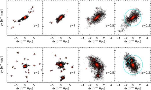
Evolution of dark matter (N-body) particle distribution around the region of subhaloes hosting mock LRGs at z = 0.3, taken from our L1000 simulation run. The upper row panels are for the region around the host halo of the brightest LRG among single-LRG systems (the host halo mass Mvir = 8.42 × 10¹⁴ h−1 M⊙), systems which host only single LRG inside in the z = 0.3 output, while the lower row panels are the most massive host halo among systems hosting one central and three satellite LRGs (Mvir = 1.44 × 10¹⁵ h−1 M⊙). The dot symbols in each panel are member particles in the halo regions at z = 2 or the subhalo region(s) at lower redshifts. The red colour particles are 30 per cent innermost particles of each halo at z = 2 and selected based on our abundance matching method between the progenitor haloes and the LRG-host subhaloes at z = 0.3 to reproduce the observed number density of SDSS LRGs (see text for details). Then we trace where the red colour particles are distributed in each subhalo region at lower redshift. By matching the red colour particles to central and satellite subhaloes in each host halo of z = 0.3 output, we can define locations of each LRG in a host halo at z = 0.3; if a subhalo at z = 0.3 contains more than 50 per cent of the red colour particles of a progenitor halo, we define it as an LRG-host subhalo. The upper row panels show the case that 11 progenitor haloes of LRGs are formed at z = 2, and then are merged at lower redshift, forming one central LRG in the host halo at z = 0.3. The lower row panels show that 24 progenitor haloes at z = 2 form one central LRG and three satellite LRGs in the host halo at z = 0.3. The blue circles in the panel of z = 0.3 show the positions of mock LRGs. The size of each circle is proportional to |$M_{\rm sub}^{1/3}$|, where Msub is the subhalo mass.
However, we need to a priori determine some model parameters before implementing to the simulation halo/subhalo catalogues: the formation redshift of LRG-progenitor haloes, zform = 2, and the fractions ‘30’ or ‘50 per cent’ for the star particles or the matching particles, respectively. Rather than exploring different combinations of the model parameters to have a better fit to the SDSS measurements, we will below study the ability of our mock catalogue to predict various statistical quantities of LRGs, by employing our fiducial choices of the parameters (zform = 2, fstar = 0.3 and fmatch = 0.5). In Appendix A, we study how variations of the model parameters change the mock catalogue. The brief summary of the results is the change of each parameter affects only the small-scale clustering signals, which are sensitive to the fraction of satellite LRGs, and does not largely change the clustering signals at large scales in the two-halo regime.
In our method, central and satellite subhaloes are populated with LRG galaxies under a single criterion: if a subhalo at z = 0.3 is a descendant of the z2-halo, the subhalo is included in the matched sample. On the other hand, the standard abundance matching method often uses different mass proxies of central and satellite subhaloes when matching subhaloes to the target galaxies (in the order of their stellar masses or luminosities). For instance, the mass of a central subhalo is assigned by a maximum circular velocity of the bounded N-body particles, computed from the output at the target redshift (z = 0.3 in the LRG case), while the mass of a satellite subhalo is assigned by the maximum circular velocity from the simulation output at the ‘accretion’ epoch before the subhalo started to accrete on to the main host halo (Conroy et al. 2006), which allows one to estimate the mass of each satellite subhalo before being affected by the tidal stripping during penetrating the main halo. Thus the standard abundance matching method is computationally more expensive in a sense that it requires many simulation outputs at different redshifts in order to trace the accretion/assembly history of each subhalo. To be fair, we below compare our method with the standard abundance matching method for some statistical quantities of LRGs.
Some of the LRG-host haloes at z = 0.3, especially massive haloes, contain multiple LRG subhaloes in our mock catalogue (see the example in the lower panel of Fig. 1). We often call such systems ‘multiple-LRG systems’ in the following discussion (also see Reid & Spergel 2009; Hikage et al. 2012b). We refer to the LRG-host haloes, which host only one LRG inside, as ‘single-LRG systems’. The average halo masses for the single- and multiple-LRG systems are found from the L1000 run to be |$\bar{M}_{\rm vir}=4.8\times 10^{13}$| and 1.5 × 10¹⁴ h−1 M⊙, respectively. The fraction of the multiple-LRG systems among all the LRG-host haloes is about 8 per cent in the L1000 run. Because we assumed that most stars of each LRG are formed until z = 2 and the total stellar mass scales with the mass of z2-halo, we define the brightest LRG (BLRG) in each multiple-LRG system by the LRG subhalo that corresponds to the most massive z2-halo among all the progenitor z2-haloes in the system, while we call the smallest z2-halo the faintest LRG (FLRG). Note that we also refer to an LRG in a single-LRG system as BLRG. A BLRG in a single-LRG system is not necessarily a central galaxy in the parent halo at z = 0.3 (in other words, the central subhalo does not correspond to any LRG-progenitor halo at z = 2). Similarly, a central LRG in a multiple-LRG system is not necessarily a BLRG, i.e. the most massive z2-halo, although the central subhalo is the most massive subhalo in the parent halo by definition.
Table 1 summarizes properties of the LRG-host haloes computed from the L1000 and L300 mock catalogues. To estimate statistical uncertainties of each quantity, we divided the L1000 catalogue into 27 subvolumes (the side length of each subvolume is 333 h−1 Mpc) and computed the mean and rms of the quantity.11 Hence the error quoted for each entry of the L1000 run corresponds to the sample variance scatter for a volume of [333 h−1 Mpc]3. The L1000 result with the error bar can be compared with the L300 result, because of the similar volumes of the subdivided L1000 catalogue and L300 run (3333 and 3003 [h−1 Mpc]3, respectively). The L1000 and L300 results agree with each other to within 2σ for the quantities except for the fraction of satellite LRGs for all the LRG-host haloes. The disagreement for the satellite LRG fraction is probably due to the numerical resolution, because the L1000 simulation may miss some less-massive LRG-progenitor haloes at z = 2, which are identified in the L300 run, due to lack of the numerical resolution and such small z = 2 haloes preferentially become satellite LRGs at z = 0.3 (also see below and Appendix A).
Summary of properties of LRG-host haloes, computed from the mock LRG catalogue in the L1000 and L300 runs (see text for details). Here we consider all LRG-host haloes and the single- and multiple-LRG haloes that host only one or multiple LRG(s) inside, respectively. |$\bar{M}_{\rm vir}$| and |$\bar{R}_{\rm vir}$| are the average virial mass and radius of the host haloes (without any weight). fsat-LRG is the fraction of haloes that have satellite LRG(s) among all the LRG-host haloes in either single- or multiple-LRG haloes (each row). Note that fsat-LRG for multiple-LRG systems is unity by definition since the haloes have satellite LRG(s). |$q_{\rm cen}^{\rm BLRG}$| is the fraction of haloes that host its BLRG as a central galaxy among all the host haloes, where BLRG is the brightest LRG, the most massive LRG-progenitor halo at z = 2, compared to other LRG subhalo(es) in the same host halo at z = 0.3. Note that, for the single-LRG hosts, we call the LRG as the BLRG. |$q_{\rm cen}^{\rm FLRG}$| is the fraction of haloes that host FLRG as a central LRG, where FLRG is the faintest LRG, the smallest LRG-progenitor halo, in each multiple-LRG halo. The error bars quoted for the L1000 mock are the standard deviation computed from the 27 divided subvolumes of L1000 mock each of which has volume of 3333 [h−1 Mpc]3. Hence, the L1000 results with the errors in each row can be compared with the L300 mock results, which has comparable volume of 3003 [h−1 Mpc]3. For comparison, we also quote the measurement results derived from the SDSS DR7 LRG catalogue in Hikage et al. (2012b), where the error bars are ±68 per cent confidence ranges (see text for details).
| Type of LRG-host haloes | Total number | |$\bar{M}_{\rm vir}\,(10^{13}h^{-1}\,\mathrm{M}_{\odot })$| | |$\bar{R}_{\rm vir}\, (h^{-1}\,{\rm Mpc})$| | fsat-LRG | |$q_{\rm cen}^{\rm BLRG}$| | |$q_{\rm cen}^{\rm FLRG}$| |
|---|---|---|---|---|---|---|
| All LRG-host haloes | ||||||
| L1000 | 91 090 | 5.64 ± 0.11 | 0.804 ± 0.004 | 0.0988 ± 0.0054 | 0.959 ± 0.004 | – |
| L300 | 2403 | 5.66 | 0.806 | 0.119 | 0.956 | – |
| Single-LRG haloes | ||||||
| L1000 | 83 891 | 4.81 ± 0.08 | 0.776 ± 0.004 | 0.0215 ± 0.0028 | 0.979 ± 0.003 | – |
| L300 | 2166 | 4.74 | 0.772 | 0.0226 | 0.977 | – |
| Hikage et al. (2012a) | 87 889 | 3.7 ± 0.4 | 0.77 ± 0.03 | 0.24 ± 0.18 | 0.76 ± 0.18 | – |
| Multiple-LRG haloes | ||||||
| L1000 | 7199 | 15.2 ± 0.8 | 1.13 ± 0.02 | 1.00 | 0.735 ± 0.025 | 0.207 ± 0.023 |
| L300 | 237 | 14.0 | 1.11 | 1.00 | 0.764 | 0.186 |
| Hikage et al. (2012a) | 4157 | 14.6 ± 1.1 | 1.21 ± 0.03 | 1.00 | 0.63 ± 0.21 | 0.24 ± 0.13 |
In Table 1, we also compare the mock results with the measurement results from the SDSS DR7 LRG catalogue in Hikage et al. (2012b). The SDSS results were derived using the different clustering measurements, the LRG–galaxy lensing, the LRG redshift-space power spectrum and the LRG-photometric galaxy cross-correlation to constrain the properties of LRG-host haloes. To be conservative, we here quote the measurement result that has largest uncertainties among the three measurements. The table shows that the mock catalogue fairly well reproduces the SDSS results within the error bars. Although one may notice sizable disagreement for the single-LRG systems, especially for the fraction of haloes hosting satellite LRGs (fsat-LRG) or the fraction of central BLRGs (|$q_{\rm cen}^{\rm BLRG}$|), the SDSS measurements are not yet reliable for the single-LRG systems, as reflected by the large error bars and stressed in Hikage et al. (2012b). Hence, this requires a further careful study.
Fig. 1 shows snapshots of the N-body particle distribution in the L1000 run outputs at different redshifts, for the regions where multiple- or single-LRG systems are formed at z = 0.3. The figure illustrates how each LRG-progenitor halo is defined at z = 2, how the innermost particles are assigned as ‘star’ particles and how the star particles are traced to lower redshifts and how LRG-progenitor haloes merge with each other and become to reside in central and satellite subhaloes at the final redshift z = 0.3. Our method allows us to directly include the merging and assembly histories of LRG-progenitor haloes. Although the number density of LRG-host subhaloes is set to the density of LRGs as we described above, the figure shows that more LRG-progenitor haloes or subhaloes survive at higher redshift than at z = 0.3. Hence our method has a capability to study what kinds of haloes or subhaloes at higher redshift are progenitors for the SDSS LRGs (see Section 4 for a further discussion).
Fig. 2 shows how each LRG-progenitor halo at z = 2 loses or gains its mass due to mass accretion, merger and/or tidal stripping when it becomes an LRG-host subhalo at z = 0.3, computed using the catalogues of haloes and subhaloes in the z = 2 and 0.3 outputs of L1000 run. Note that the halo mass shown in the x-axis, MFoF(z = 2), is the FoF mass, the sum of FoF particles in each halo region at z = 2. First, the figure shows that we need to select the LRG-progenitor haloes at z = 2 down to a mass scale of about 6 × 10¹² h−1 M⊙. Some subhaloes for satellite LRGs lose their masses due to tidal stripping as implied in Fig. 1, while subhaloes for central LRGs gain their masses due to mass accretion and/or merger. Comparing the left- and right-hand panels manifests that multiple-LRG systems tend to reside in more massive LRG-progenitor haloes at z = 2 and become more massive LRG-host haloes at z = 0.3, and that the mass difference between subhaloes for central and satellite LRGs is larger in multiple-LRG systems, implying a larger difference between their luminosities (see Hikage et al. 2012b, for a similar discussion).
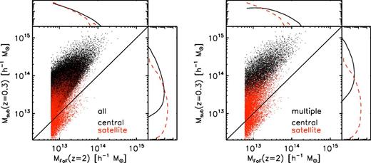
Comparison between masses of the LRG-progenitor haloes at z = 2 and the LRG-host subhaloes at z = 0.3, computed from the L1000 run, where each progenitor halo and subhalo are matched based on our method (see Fig. 1). The left- and right-hand panels show the results for all the LRG-host haloes and the multiple-LRG systems, respectively. The black and red points are for central and satellite LRGs, respectively. Note that the central LRG subhalo is a smooth component of the parent halo at z = 0.3. The line in each panel shows the case that the progenitor halo does not either gain or lose its mass at z = 0.3: Msub(z = 0.3) = MFoF(z = 2). The figure shows that satellite LRGs preferentially reside in less massive progenitor haloes at z = 2, some subhaloes for satellite LRGs lose their masses due to tidal stripping when accreting into more massive haloes and subhaloes for central LRGs gain their masses due to merger. The upper and right-hand side panels in each plot are the projected distributions for central and satellite LRGs along the y- or x-axis direction, respectively.
Thus our method is primarily based on the masses of LRG-progenitor haloes at z = 2 (see Fig. 2) and the connection with central and satellite subhaloes in the parent haloes at z = 0.3. On the other hand, LRGs in the SDSS catalogue are selected based on the magnitude and colour cuts from the SDSS imaging data (primarily gri), and are not necessarily a stellar-mass-selected sample, although their stellar masses are believed to have a tight relation with the host halo masses. Nevertheless, we will show below that the mock catalogue perhaps surprisingly well reproduces the different SDSS measurements.
Since LRGs in our mock catalogue reside in relatively massive haloes at z = 2, with masses MFoF ≳ 6 × 10¹² h−1 M⊙ (Fig. 2), as well as in massive parent haloes at z = 0.3, our method does not necessarily require a high-resolution simulation. A simulation with 10243 particles and 1 h−1 Gpc size on a side seems sufficient, which allows for a relatively fast computation of the N-body simulation as well as an accurate estimation of statistical quantities of LRGs. This is not the case if one wants to work on the abundance matching method for less massive galaxies or more general types of galaxies (e.g. Trujillo-Gomez et al. 2011; Reddick et al. 2012; Masaki et al. 2013).
3 RESULTS: COMPARISON WITH THE SDSS LRG MEASUREMENTS
3.1 Halo occupation distribution and properties of satellite LRGs
First, we study the HOD for LRGs in Fig. 3, where the HOD gives the average number of LRGs that the haloes at z = 0.3 host as a function of host-halo mass. Here we consider the HODs for central and satellite LRGs which reside in central and satellite subhaloes in the LRG-host haloes, respectively. Again we should emphasize that our method does not assume any functional forms for the HODs, unlike done in the standard HOD method, and rather allows us to directly compute the HODs from the mock catalogue. Even if LRG-progenitor haloes are selected from haloes at z = 2 by a sharp mass threshold, our mock catalogue naturally predicts that the central HOD has a smoother shape around a minimum halo mass, as a result of their merging and assembly histories from z = 2 to 0.3. To be more precise, the central HOD is smaller than unity (〈Ncen〉 < 1) for host haloes with Mvir ≲ 1014 h−1 M⊙, meaning that only some fraction of the haloes host a central LRG. On the other hand, most of massive haloes host at least one LRG and can host multiple LRGs inside. Conversely, the fraction of massive haloes, which do not host any LRG, is 1.3 per cent for haloes with masses Mvir ≥ 1 × 10¹⁴ h−1 M⊙, while all haloes with Mvir ≥ 2 × 10¹⁴ h−1 M⊙ have at least one LRG inside.
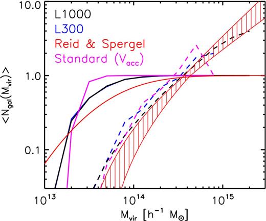
The HOD for LRGs as a function of parent halo mass, measured from our mock catalogue. Our mock catalogue has an assignment of each LRG to central or satellite subhaloes in a parent halo at z = 0.3 (see Fig. 1), thereby allowing us to compute the HODs for central (solid curve) and satellite (dashed) LRGs. The black and blue curves are the results from the L1000 and L300 runs, respectively, where the L300 run is a higher resolution run with a small box size, 300 h−1 Mpc (see text for details). The red curves show the SDSS measurements, taken from RS09. RS09 fixed the function form of central HOD, and then constrained the satellite HOD from the SDSS LRG catalogue using the CiC technique. The hatched region is the range allowed by varying each model parameter of the satellite HOD within its 1σ confidence range. The mock catalogue well reproduces the SDSS measurements, including the shape of central HOD around the cut-off mass scale as well as the slope and amplitude of satellite HOD, without employing any free parameter to adjust after the abundance matching. The magenta lines show the HODs from the LRG mock catalogue generated using the standard abundance matching method in Conroy et al. (2006) (also see text for the details).
On the other hand, the satellite HOD in RS09 is almost perfectly recovered by our mock catalogue, where RS09 assumed the functional form for the satellite HOD to be given by 〈Nsat(M)〉 = 〈Ncen(M)〉[(M − Mcut)/M1]α and then constrained the parameters (Mcut, M1, α) from the SDSS LRG catalogue. The hatched region is the range at each host-halo mass bin that is allowed by varying the model parameters within the 1σ confidence regions. Our results confirm that parent haloes of ∼1015 h−1 M⊙ have up to several LRGs inside, as first pointed out in RS09. The L300 result, the simulation result with higher spatial resolution, gives similar results to the L1000 results, showing that the numerical resolution is not an issue in studying the satellite HOD. Even though SDSS LRGs are selected by the magnitude and colour cut, not by their masses, our method seems to capture the origin of SDSS LRGs; mass-selected haloes at z ∼ 2 are main progenitors of LRGs, and their subsequent assembly and merging histories determine where LRGs are distributed within the host haloes at lower redshift.
Furthermore, to be comprehensive, we also compare our method with the standard abundance matching method in Conroy et al. (2006). In this method, the mass proxy of each subhalo is assigned by the maximum circular velocity Vcir computed from the member N-body particles. More specifically, the central subhalo mass is assigned by Vcir at the LRG redshift z = 0.3, while the satellite subhalo mass is estimated by Vcir from the simulation output at its ‘accretion’ epoch when the subhalo started to accrete on to the parent halo at z = 0.3 (more exactly, the circular velocity is estimated from the last output when the ‘subhalo’ was identified as an ‘isolated’ halo before the accretion; see also Masaki et al. 2013). This prescription for satellite subhaloes allows for a better assignment of the subhalo mass so that it avoids the effect by tidal stripping during accreting on to the parent halo. We use the L300 run outputs at 44 different redshifts from z = 10 to trace the merging and assembly history of each subhalo till z = 0.3. Then, assuming that the stellar masses of LRGs trace the subhalo masses, we match the z = 0.3 subhaloes to LRGs in descending order of the mass proxies (Vcir) until the number density is closest to the target value, |$\bar{n}_{\rm LRG}=10^{-4}\,(h\,{\rm Mpc}^{-1})^3$|. The curves labelled as ‘Standard (Vacc)’ show the central and satellite HODs measured from the mock catalogue of the Vcir-based abundance matching method. The satellite HOD is in a nice agreement with our method, while the central HOD from the abundance matching method displays a sharper cut-off than in our method. Again we do not yet know the genuine cut-off feature of the central HOD due to lack of the measurement constraints. We will below further compare our method with the abundance matching method for other statistical quantities of LRGs.
One motivation of this paper is to understand the physics of the non-linear redshift-space distortion, i.e. the Finger-of-God (FoG) effect, in the redshift-space power spectrum of LRGs. The FoG effect is caused by internal motion of satellite LRG(s) in LRG-host haloes (Hikage, Takada & Spergel 2012a; Hikage et al. 2012b). In the following, we study several quantities relevant for the FoG effect: the fraction of satellite LRGs, the radial profile of satellite LRGs inside the parent haloes and the internal velocities of satellite LRGs (see Hikage et al. 2012a, for details of the theoretical modelling).
Fig. 4 shows how much fraction of LRG-host haloes at z = 0.3 host satellite LRG(s) inside, as a function of the halo mass. Note that we excluded haloes that do not host any LRG in this statistics, but included the single-LRG systems hosting one LRG as a satellite galaxy when computing the numerator of the fraction (in this case, the central subhalo of the parent halo does not correspond to any LRG-progenitor halo at z = 2). The error bars around the solid curve are Poisson errors, estimated using the number of haloes in each mass bin. The figure shows that more massive haloes have a higher probability to host satellite LRG(s). About 20 per cent of parent haloes with Mvir ≃ 1014 h−1 M⊙ host satellite LRG(s).
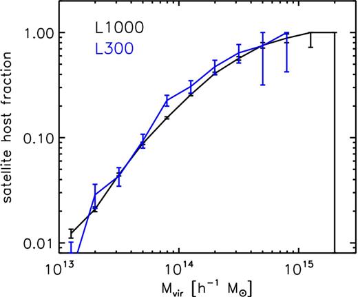
The fraction of haloes hosting satellite LRG(s) inside as a function of halo mass, computed by using all the LRG-host haloes at z = 0.3 in the L1000 and L300 runs.
We naively expect that BLRG, the most massive LRG-progenitor halo at z = 2 among LRG-progenitor halo(es) accreting on to the same parent halo at z = 0.3, becomes a central galaxy. The solid curves in Fig. 5 show the fraction of BLRGs to be a satellite galaxy in LRG-host haloes at z = 0.3 as a function of the halo mass, computed using all the LRG-host haloes. For haloes with Mvir ≳ 1014 h−1 M⊙, there is up to 10 per cent probability for its BLRG to be a satellite galaxy.
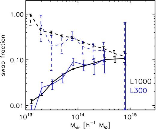
The solid curves show the fraction of the parent haloes hosting the BLRG as a satellite galaxy, among all the LRG-host haloes. Here the BLRG is the most massive LRG-progenitor halo at z = 2 among all the progenitor haloes which become to reside in the same LRG-host halo at z = 0.3. The dashed curves are the similar fraction of LRG-host haloes with satellite BLRG, but computed using only the multiple-LRG systems. The error bars are computed from the number of haloes in each mass bin assuming Poisson statistics.
The dashed curves are the similar fraction, but computed using only the multiple-LRG systems. This sample is intended to compare with the recent result in Hikage et al. (2012b) (also see Table 1). In this case, the fraction of satellite BLRGs is higher for host haloes with smaller masses, with larger error bars. This can be explained as follows. Most of low-mass host haloes with masses ≲1014 h−1 M⊙ are single-LRG systems as can be found from Fig. 3, and only a small number of such haloes are multiple-LRG systems, causing larger Poisson error bars at each mass bin. We have found from the simulation outputs that such low-mass haloes of multiple-LRG systems (mostly the systems with two LRGs) tend to display a bimodal mass distribution due to ongoing or past major merger, where the BLRG and other (mostly central) LRG tend to have the small mass difference. As a result, such low-mass multiple-LRG systems have a higher chance to host the BLRG as a satellite LRG. On the other hand, the fraction of haloes with satellite BLRG converge to the solid curve with increasing the host-halo mass, because most of such massive haloes are multiple-LRG systems. For multiple-LRG systems with mass of Mvir ≃ 1014 h−1 M⊙, about 30 per cent of BLRGs are satellite galaxies.
Recently, Hikage et al. (2012b) studied the multiple-LRG systems defined from the SDSS DR7 catalogue by applying the CiC technique as well as the FoF group finder method to the distribution of LRGs in redshift space. Then they used the different correlation measurements, the redshift-space power spectrum, the LRG–galaxy lensing and the cross-correlation of LRGs with photometric galaxies, to study properties of satellite LRGs. From the lensing analysis, they found that the multiple-LRG systems has a typical halo mass of Mvir ≃ 1.5 × 10¹⁴ h−1 M⊙ (with a roughly 10 per cent statistical error), and that 37 ± 21 per cent of BLRGs in the multiple-LRG systems appear to be satellite galaxies.12 Our mock catalogue shows a fairly good agreement with the SDSS results, for the average halo mass and the fraction of satellite BLRGs (also see Table 1).
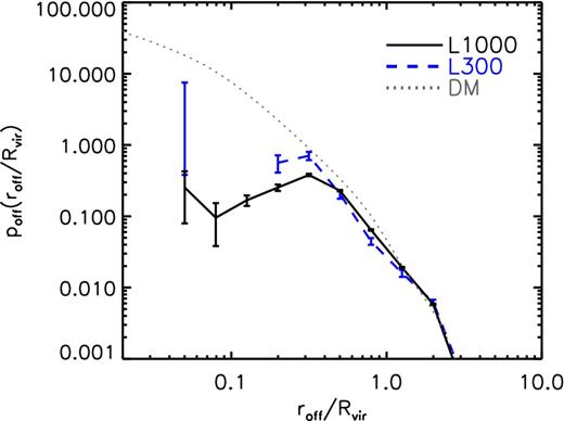
The average radial profile of satellite LRG host subhaloes, obtained by stacking the positions of satellite LRGs in all the LRG-host haloes with satellite LRG(s), as a function of radius relative to the virial radius of each parent halo. The mean mass of the LRG-haloes used in this calculation is Mvir ≃ 1.31 or 1.24 × 10¹⁴ h−1 M⊙ for the L1000 or L300 runs, while the mean virial radius is Rvir ≃ 1.07 or 1.06 h−1 Mpc, respectively. For comparison, the upper dotted curve shows the profile of dark matter averaged for the same host haloes with an arbitrary amplitude. The error bars at each radial bin are estimated by first dividing LRG-host haloes into 27 subsamples (27 subvolumes) and then computing variance of the number of satellite LRGs at the radial bin. The typical off-centre radius for satellite LRGs appears to be about 400 h−1 kpc.
Fig. 7 shows the average radial profile of internal motions of satellite LRGs in the parent haloes, where the bulk motion of each parent halo (the average velocity of N-body particles belonging to the smooth component of the halo) is subtracted from the velocity of each LRG-host subhalo. We considered only the host haloes with satellite LRG(s) as in Fig. 6. The curves, labelled as 〈voff, r〉, are the average radial velocities for all the satellite LRGs with respect to the halo centre. The average velocity is negative, reflecting the coherent infall motion towards the halo centre, and the infall velocity is larger with increasing radius up to the virial radius. The average radial velocity becomes zero on average at the halo centre. These support that the LRG-host subhalo approaches to the halo centre due to dynamical friction. On the other hand, the curves, labelled as σoff, r, are the average velocity dispersions of satellite LRGs. The velocity dispersion has greater amplitudes with decreasing the radius, reaching to σoff, r ≃ 500 km s−1. For comparison, the horizontal dotted line shows the average virial velocity dispersion, |$\sigma _{\rm vir}\equiv \sqrt{GM_{\rm vir}/2R_{\rm vir}}=521\,{\rm km\,s^{-1}}$|, among the satellite LRG-host haloes in the L1000 run. The combination of 〈voff, r〉 and σoff, r implies that satellite LRGs gradually approach to the halo centre due to dynamical friction and have an oscillating motion around the halo centre. Again the amplitude of the velocity dispersion, σoff, r ≃ 500 km s−1, is in nice agreement with the recent measurement in Hikage et al. (2012b), where they found the velocity dispersion of about 500 km s−1 for satellite LRGs in the multiple-LRG systems by combining the different correlation measurements from the SDSS DR7 LRGs. In Section 3.4 we will further discuss how satellite LRG subhaloes affect the redshift-space power spectrum due to the FoG effect.
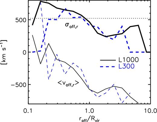
The average radial velocity of satellite LRGs, 〈voff, r〉, with respect to the halo centre in each LRG-host halo, computed by using all the LRG-host haloes with satellite LRG(s) as in the previous figure. The negative 〈voff, r〉 means a coherent infall towards the halo centre. The upper curves show the average radial velocity dispersion around the coherent infall, σoff, r. For the comparison, the dotted line shows the average velocity dispersion expected from virial theorem, |$\sigma _{\rm vir}=\sqrt{GM_{\rm vir}/2R_{\rm vir}}$|. The combination of 〈voff, r〉 and σoff, r implies that satellite LRG(s) sink towards the halo centre due to dynamical friction, and then have an oscillating motion around the halo centre with the velocity dispersion of ≃500 km s−1.
3.2 Projected correlation function
In Fig. 8, we compare the projected correlation function measured from our LRG mock catalogue with the SDSS measurements (Zehavi et al. 2005; Masjedi et al. 2006). In the SDSS measurements, Zehavi et al. (2005) used an LRG sample in the magnitude range of −23.2 < Mg < −21.2 and with the mean redshift 〈z〉 ≃ 0.3. Masjedi et al. (2006) used the same sample to extend the measurement down to very small scale, below R = 500 h−1 kpc, by taking into account various observational effects such as the fibre collision. Note that the cosmological model employed in the measurement is slightly different from the model we assumed for our simulations. The figure shows that our mock catalogue remarkably well reproduces the projected correlation function of LRGs, to within 30 per cent accuracy in the amplitude, over a wide range of separation radii, which arise from correlations between LRGs within the same host halo and in different host haloes, the so-called one- and two-halo regimes, respectively.13 Comparing the results for the L1000 and L300 runs reveals that the correlation function for L1000 has a smaller amplitude at R < 0.7 h−1 Mpc than that for L300. Thus the L1000 run implies a systematic error due to the lack of numerical resolution at the small scales. The L300 result shows a better agreement with the SDSS measurement in Masjedi et al. (2006). The small-scale clustering arises mostly from correlation between LRGs in the same multiple-LRG system, so that numerical resolution seems important to resolve these small subhaloes (also see below for a further discussion).
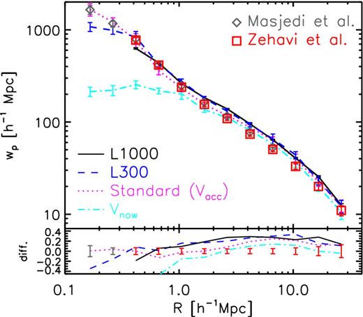
Top panel: projected autocorrelation function of LRGs, wp(R), as a function of the projected distance R. The solid and dashed curves show the results from our mock catalogues in the L1000 and L300 runs, respectively. The error bars are estimated using the measurements from eight subdivided volumes of each simulation volume, where the error bars are estimated by dividing the standard deviation by |$\sqrt{8}$|. Hence the error bars are the statistical scatters for a volume of (1 h−1 Gpc)3 or (300 h−1 Mpc)3, respectively. The square and diamond symbols are the correlation functions measured from the SDSS catalogue of LRGs at z ∼ 0.3, taken from Zehavi et al. (2005) and Masjedi et al. (2006), respectively. For comparison, the magenta, dotted curve shows the result from the standard abundance matching method as in Fig. 3. Furthermore, we also show the prediction obtained if we used the maximum circular velocity at the LRG redshift z = 0.3, instead of the accretion epoch, for the satellite subhaloes in the abundance matching method (see text for the details). Bottom panel: the fractional differences of the model predictions compared to the SDSS measurements.
As in Fig. 3, the dotted curve gives the result from the standard abundance matching method, which shows almost similar level agreement with the SDSS measurements to our method. Thus, since the abundance matching method rests on the higher resolution L300 outputs at 44 different redshifts (in our case), our method can provide a much computationally cheap, alternative approach to making a mock catalogue of LRGs. Furthermore, for comparison, the dot–dashed curve shows the correlation function, if the abundance matching is done by using the maximum circular velocity at the LRG redshift (z = 0.3) for each satellite subhalo as its mass proxy, instead of the velocity at the accretion epoch. The result shows a significant discrepancy with the SDSS measurements or our method and the standard abundance matching method, especially at small radii. The disagreement means that the circular velocity at z = 0.3 is not a good mass proxy for satellite subhaloes when matching the subhaloes to LRGs, because it misses satellite subhaloes in the multiple-LRG systems. To be more precise, mass (circular velocity) of each satellite subhalo tends to be underestimated due to the tidal stripping, then tends to be not selected by the abundance matching, and instead other isolated, less-massive haloes tend to be selected. This reduces the clustering signals at small scale due to less contribution from satellite subhaloes and also reduces the clustering signal at large scales due to a smaller bias for such low-mass haloes. Thus detailed features of the correlation functions at different scales are sensitive to the contribution of satellite LRGs as well as the low-mass threshold of central HOD in Fig. 3 (also see Appendix A). Note that an explicit implementation of the abundance matching method to LRGs is the first time, and the result in Fig. 8 highlights the importance of proper assignment of subhalo masses in the abundance matching method.
3.3 LRG–galaxy weak lensing
Fig. 9 shows that the average mass profile measured for all LRGs in the mock catalogue is in good agreement with the SDSS measurement in Mandelbaum et al. (2013), to within 30 per cent level in the amplitude. Note that, to obtain the average mass profile from our mock catalogue, we stacked all N-body particles around all the LRG-host subhalo in the simulation, including the particles outside dark matter haloes. The lensing signal at the radii smaller than about 1 h−1 Mpc arises from the mass distribution within the same halo, while the signal at the larger scale arises from the mass distribution surrounding the host haloes – the one- and two-halo terms, respectively (e.g. see Oguri & Takada 2011). The mock catalogue well reproduces both the signals of different scales. The average halo mass inferred from the SDSS measurement is |$\bar{M}_{\rm vir}\simeq 4.1\times 10^{13}\,h^{-1}\,\mathrm{M}_{\odot }$| (Hikage et al. 2012b) (see also Table 1). Furthermore, the standard abundance matching method shows a similar level agreement with the SDSS measurement, similarly to Fig. 8. Hikage et al. (2012b) also used the SDSS LRG catalogue to study the weak lensing for the multiple-LRG systems. When making the lensing measurements, they used three different proxies for the halo centre of each multiple-LRG system, the BLRG, FLRG and the arithmetic mean position of member LRGs (hereafter ‘Mean’). By comparing the lensing signals for the different centres, they constrained the average radial profiles of satellite BLRGs and FLRGs, finding about 400 h−1 kpc for a typical offset radius from the true centre. Fig. 10 shows that the mock catalogue predictions are in remarkably good agreement with the SDSS measurements for the different centres. Since these lensing signals are from the exactly same catalogue of the multiple-LRG systems, the differences between the different measurements should be due to the off-centring effects of the chosen centres. As nicely shown in Hikage et al. (2012b), the lensing signals for the BLRG and FLRG centres can be well explained by a mixture of the central and satellite BLRGs or FLRGs in the sample. The lensing signals for the FLRG centre have smaller amplitudes due to the larger dilution effect because of a larger fraction of satellite (off-centred) FLRGs than in the BLRG centres. On the other hand, the Mean centre does not have any galaxy (subhalo) at its position, and therefore the Mean centre always has an off-centring effect from the true centre in each LRG system. This causes decreasing powers of the lensing signal at the smaller radii than the typical off-centre radius. The lensing signals at some radii for the FLRG and Mean centres show some discrepancy from the mock catalogue, but we do not think that the disagreement is significant. The average masses inferred from the SDSS measurement and the mock catalogue for the multiple-LRG haloes agree within about 30 per cent; |$\bar{M}_{\rm vir}\simeq 1.46$| or 1.52 × 10¹⁴ h−1 M⊙, respectively (also see Table 1).
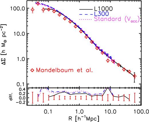
Top panel: the average surface mass density profile around LRGs, which is an observable of the LRG–galaxy weak lensing. The solid and dashed curves are the results of our mock catalogue, obtained by stacking N-body particles around all the LRG-host subhaloes in the L1000 and L300 runs, respectively. The error bars are estimated using the measurements from 27 subsamples of LRG-host subhaloes. The data with error bars show the SDSS measurements in Mandelbaum et al. (2013). As in Figs 3 and 8, we also show the result obtained from the standard abundance matching method (dotted curve). Bottom panel: the fractional differences of the model predictions compared to the measurement.
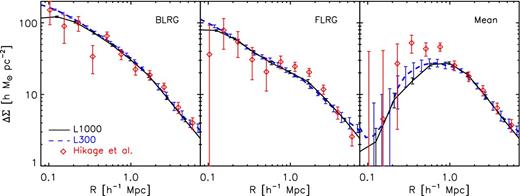
The average surface mass profiles for the multiple-LRG systems. The different panels show the results obtained by taking the different centres in each multiple-LRG halo: the BLRG, the FLRG and the centre-of-mass of different LRGs or the arithmetic mean positions of member LRGs (Mean) in the left-hand, middle and right-hand panels, respectively. The data with error bars show the SDSS measurements for the multiple-LRG systems in Hikage et al. (2012b).
As can be shown in Figs 8–10, our mock catalogue of LRGs well reproduces both the SDSS measurements for the autocorrelation function of LRGs and the LRG–galaxy weak lensing simultaneously. As recently discussed in Neistein & Khochfar (2012) (also see Neistein et al. 2011), the abundance matching method has a difficulty to reproduce these measurements with the same model, although they considered the spectroscopic sample of SDSS galaxies, rather than focused on LRGs. Thus the agreements of our mock catalogue show a capability of our method to predict different statistical quantities of LRGs by self-consistently modelling, rather than assuming, the fractions of satellite LRGs among different haloes and the radial distribution of satellite LRGs in the parent haloes (also see Masaki et al. 2013, for a recent development on the extended abundance matching method based on the similar motivation).
3.4 Redshift-space power spectrum of LRGs
Another observable we consider is the redshift-space power spectrum of LRGs. The FoG effect due to internal motion of galaxies is one of systematic errors to complicate the cosmological interpretation of the measured power spectrum. The FoG effect involves complicated physics inherent in the evolution and assembly processes of galaxies, so is very difficult to accurately model from the first principles. One way to reduce the FoG contamination is to remove satellite galaxies from the region of each multiple-LRG system, and to keep only one galaxy (LRG in our case), ideally the central galaxy, because the central galaxy is supposed to be at rest with respect to the parent halo centre and does not suffer from the FoG effect. For example, Reid et al. (2010) developed a useful method for this purpose; first, reconstruct the distribution of haloes from the measured distribution of LRGs by identifying multiple-LRG systems based on the CiC and FoF group finder method, and then keep only one LRG for each multiple-LRG system. However, the chosen LRG is not necessarily the central galaxy (more exactly, they used, as the halo centre proxy, the arithmetic mean of member LRGs or the centre-of-mass of different CiC groups without any luminosity or mass weighting), so there may generally remain a residual FoG contamination in the measured LRG power spectrum as pointed out in Hikage et al. (2012b).
In the left-hand panel of Fig. 11, we study the FoG effect on the redshift-space power spectrum, caused by the off-centring effect of LRGs in our mock catalogue. Following the method in Reid et al. (2010) and Hikage et al. (2012b), we study the redshift-space power spectrum for LRG-host haloes, instead of the power spectrum for LRGs. To compute the power spectrum of haloes, we need to specify the halo centre in each LRG-host halo. For single-LRG systems, we use the LRG position as the halo centre proxy. For multiple-LRG systems, we employ different proxies of halo centre for each system as done in Fig. 10 for the LRG–galaxy lensing; BLRG, FLRG or the arithmetic mean (Mean), where the Mean centre is computed in redshift space taking into account redshift-space distortion due to peculiar velocities of LRG subhaloes. The figure shows the angle-averaged redshift-space power spectra for the different centres, relative to the power spectrum for the mass centre of each LRG-host halo (the mass centre of N-body particles of the host halo). Note that, for the power spectrum measurement, we used the exactly same catalogue of LRG-host haloes, and the different power spectra differ in the chosen halo centre of each multiple-LRG system. Hence, the difference between the different spectra should be from the off-centring effects of the chosen centres in the multiple-LRG systems. Interestingly, the spectra for BLRG, FLRG and Mean centres all show smaller amplitudes with increasing wavenumber, as expected in the FoG effect. To be more precise, the power spectrum of FLRG centre shows the strongest FoG effect, because a larger fraction of FLRGs are satellite galaxies than BLRGs (see Table 1). These results can be compared with fig. 2 in Hikage et al. (2012b). It can be found that the mock catalogue qualitatively reproduces the SDSS measurements: the spectra of BLRG and Mean centres are similar, and the spectrum for FLRG shows the stronger FoG suppression.
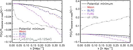
The angle-averaged redshift-space power spectra for the LRG-host haloes at z = 0.3, computed from the L1000 run. The different curves show the fractional differences of the power spectra using different proxies of each LRG-host halo position in the power spectrum estimation, relative to the power spectrum for the mass centre as the halo position. Left-hand panel: the dotted, dashed and dot–dashed curves are the results when using different halo centre proxies for each multiple-LRG system; the arithmetic mean position of the member LRGs in redshift space (Mean), BLRG or FLRG as in Fig. 10. Note that we use the LRG position as the halo centre for each single-LRG system. Thus the differences between the different spectra arise only from the different positions of multiple-LRG systems in redshift space, to be compared with Hikage et al. (2012b). The different power spectra show decreasing amplitudes with increasing wavenumber, which is caused by the non-linear redshift-space distortion, the so-called Finger-of-God effect, due to the internal motions of the chosen halo centres in LRG-host haloes. For comparison, we also show the power spectrum measured using the potential minimum of each LRG-host halo, where the potential minimum is the mass density peak of the smooth component of the halo that is likely to host the central galaxy. For comparison, the three dots–dashed curve shows the effect on the real-space matter power spectrum caused by massive neutrinos assuming the total neutrino mass mν, tot = 0.125 eV. Right-hand panel: similar to the left-hand panel, but the power spectrum using all the LRGs is added (the three dots–dashed curve). The power spectrum includes contributions from multiple LRGs in the same halo. The shot noise contamination due to the different number densities of the LRG-host haloes and the LRG-host subhaloes is properly subtracted to have a fair comparison.
Fig. 11 also shows the power spectrum using the potential minimum as the centre of each halo. We define the potential minimum as the mass density peak of smooth component: the central subhalo position, in each LRG-host halo. In this part of the analysis, the power spectrum is measured by using the position of a central galaxy in each host halo. Again note that BLRG is not necessarily a central subhalo (galaxy) as shown in Fig. 5. The power spectrum for the potential minimum has a smaller amplitude than that of the mass centre of host halo, implying that the potential minimum is moving around the mass centre in each halo. Comparing the spectra for the potential minimum and the BLRG centre shows that the BLRG spectrum has a smaller amplitude than the spectra for the potential minimum or the mass centre by a few per cent in the fractional amplitude up to k ≃ 0.3 h Mpc−1. The few per cent level FoG contamination would be okay for a current accuracy of the power spectrum measurement, but will need to be carefully taken into account for a higher precision measurement of upcoming redshift surveys. For comparison, the three dots–dashed curve shows the effect on the real-space matter power spectrum caused by massive neutrinos, where we assumed mν, tot ≃ 0.1 eV for the total mass of neutrinos, close to the lower limit on the neutrino mass for the inverted mass hierarchy. For the normal mass hierarchy, the lower limit on the total mass is about 0.05 eV, and the amount of the suppression is about half of the result of 0.1 eV in Fig. 11. The lowest curve in the figure shows the difference of the real-space matter power spectrum when taking account of massive neutrinos relative to the spectrum for the massless neutrino cosmology.
In the right-hand panel of Fig. 11, we also show the redshift-space power spectrum derived by using all the LRGs in the catalogue. Note that we properly subtracted the shot noise contamination from the measured power spectra by using the number densities of LRGs or LRG-host haloes. In this case, the power spectrum ratio shows greater amplitudes with increasing wavenumber rather than the FoG suppression. That is, the LRG power spectrum shows a greater clustering power or greater bias than in the LRG-host halo spectrum. The scales shown here, the scales greater than a few tens Mpc, are much larger than a virial radius of most massive host haloes and the one-halo term arising from clustering between two LRGs in the same host halo should not be significant at these scales. Hence, the greater amplitudes in the LRG power spectrum would be due to a more weight on more massive haloes, because satellite LRGs preferentially reside in more massive haloes that have larger biases. Since the effect of different linear bias should cause only a scale-independent change in the power spectrum ratio, the change in the LRG power spectrum should be from a stronger non-linear bias of such massive haloes, even though the FoG suppression should be more significant for such haloes. In fact, a combination of the perturbation theory of structure formation and halo bias model seems to reproduce such a non-trivial behaviour in the power spectrum amplitudes (Nishizawa, Takada & Nishimichi 2012). The results in the figure imply that including satellite LRGs in the power spectrum analysis complicates the interpretation of the measured power spectrum, thereby causing a bias in cosmological parameters. These subtle effects need to be well understood if we are going to use power spectrum measurements to place unbiased constraints on cosmological parameters such as the neutrino mass.
In Fig. 12, we study how the residual FoG effect varies with masses of LRG-host haloes. To study this, we divide the LRG haloes into two subsamples by masses of the LRG haloes smaller and larger than the median, and measured the fractional power spectra for each subsample relative to the halo sample. As expected, the FoG effect is larger for the subsample containing more massive haloes, because of the higher fraction of satellite BLRGs as well as the larger velocity dispersion (larger halo mass). The right-hand panel shows the similar results, but obtained only by using the single-LRG haloes. First of all, the single LRG systems have a smaller FoG effect, because of the smaller fraction of satellite BLRGs (Fig. 5 and Table 1) as well as the smaller velocity dispersions for the lower mass host haloes. Among the single-LRG haloes, more massive haloes have relatively a larger FoG contamination, but only by a few per cent at k ≲ 0.35 h Mpc−1 in the amplitude. Thus, the use of single-LRG systems may allow a cleaner interpretation of the measured power spectrum, yielding a more robust, unbiased constraint on cosmological parameters.
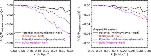
Similarly to the previous figure, but for the halved samples of LRG-host haloes. Left-hand panel: the LRG haloes are divided into two halved samples by the halo masses; one subsample is defined by haloes which have masses smaller than the median mass (‘small-half’), while the other is by haloes with masses larger than the median (‘massive-half’). The massive halo subsample shows a stronger FoG effect. Right-hand panel: similar plot, but using only the single-LRG haloes.
4 DISCUSSION AND CONCLUSION
In this paper, we have developed a new abundance-matching-based method to generate a mock catalogue of the SDSS LRGs, using catalogues of haloes and subhaloes in N-body simulations. A brief summary of our method is as follows: (1) identify LRG-progenitor haloes at z = 2 down to a certain mass threshold until the comoving number density of the haloes become similar to that of the SDSS LRGs at z = 0.3; (2) trace the merging and assembly histories of the LRG ‘star particles’, the 30 per cent innermost particles of each z = 2 LRG-progenitor halo that are gravitationally, tightly bounded particles and (3) at z = 0.3, identify the subhaloes and haloes hosting the LRG ‘star’ particles. If a subhalo at z = 0.3 contains more than 50 per cent of the star particles of any progenitor halo, we assign the subhalo at z = 0.3 as an LRG-host subhalo. We should emphasize that our method does not employ any free fitting parameter to adjust in order for the model to match the measurements, once the mass threshold of the LRG-progenitor haloes is determined to match the number density of SDSS LRGs. Thus, by assuming that a majority of stellar components of LRG is formed at z = 2, we can trace the assembly and merging histories of LRGs over a range of redshift, z = [0.3, 2]; for example, we can directly trace which LRGs become central or satellite galaxies in the LRG-host haloes at z = 0.3. The novel aspect of our approach is that the abundance matching of haloes to a particular type of galaxies (LRGs in this paper) is done by connecting the haloes and subhaloes at different redshifts (z = 2 and 0.3 in our case), while the standard method is done for the same or similar redshift to the redshift of target galaxies. In addition, central and satellite subhaloes are populated with galaxies under a single criterion: if a subhalo at z = 0.3 is a descendant of the z2-haloes, the subhalo is included. The standard abundance matching uses different quantities for central and satellite subhaloes, e.g. the circular velocities at the galaxy redshift and at the accretion epoch, respectively.
Using the mock catalogue, we have computed various statistical quantities: the HOD, the projected correlation function of LRGs, the mean surface mass density profile around LRGs (which is an observable of the LRG–galaxy weak lensing) and the redshift-space power spectrum of LRGs. We showed that the mock catalogue predictions are in a good agreement with the measurements from the SDSS LRG catalogue (Figs 3 and 8–11). Thus our method seems to capture an essential feature of LRG formation in terms of a hierarchical structure formation scenario of ΛCDM model.
In the SDSS sample, about 5 per cent of the haloes contain multiple LRGs. In our simulation, 8 per cent of the haloes contain multiple LRGs. This modest deviation may be due to our simplified assumptions. First, we assumed that LRG progenitors are formed at a single epoch, z = 2. This is too simplified assumption as LRG formation almost certainly took place over a range of redshifts. Including a broader period of formation of LRG-progenitor haloes may improve the model prediction. Secondly, although LRGs are observationally selected by magnitude and colour cuts, our definition of the LRG-progenitor haloes at z = 2 is solely based on their masses. The agreements between our mock catalogue and the SDSS measurements support that the matching based on the LRG-progenitor halo masses seems fairly reasonable to mimic a population of LRGs. However, the model may be further refined by combining masses of the progenitor haloes with other indicators when matching to LRGs. For instance, using the maximum circular velocity of each halo instead of its mass may improve the model accuracy. Another potential improvement would be to introduce some stochasticity into the relationship between halo mass and inclusion in the LRG sample. Variation in star formation histories should introduce scatter into the halo mass/galaxy luminosity relation. We have done a preliminary study where we introduce some scatter and find that this lowers the characteristic halo mass, which leads to smaller bias parameters, and obviates the disagreement between theory and observation for the projected correlation function or the lensing mass profile in Figs 8 and 9. Another simplifying assumption was our neglect of satellite subhaloes in the parent halo at z = 2 in the abundance matching procedure. We naively expect that subhaloes at z = 2 merge into central subhaloes from z = 2 to 0.3 due to dynamical friction, so we used the simplest method as the first attempt. However, including the subhaloes at z = 2 for the abundance matching may improve an accuracy of the mock catalogue. We plan to explore these improvements in a future work.
Our mock catalogue or more generally our abundance matching method offers several applications to measurements. First, Masjedi et al. (2008) showed that, by using the small-scale clustering signal and the pair counting statistics, LRGs are growing by about 1.7 per cent per Gyr, on average from merger activity from z = 1 to ∼0.3. Our method directly traces how each LRG-progenitor halo acquires the mass from other LRG-progenitor haloes by major or minor mergers from z = 2 to 0.3. Hence, we can compare the prediction of our mock catalogue with the measurement for the mass growth rate of LRGs. By using the constraint, we may be able to further improve the mock catalogue.
Secondly, our method can predict how the distribution of LRG progenitor evolves in relative to dark matter distribution as a function of redshift. Thus, our mock catalogue can be used to predict various cross-correlations of LRG positions with other tracers of large-scale structure. As one such example, in this paper, we have studied the LRG–galaxy weak lensing measured via cross-correlation of LRGs with shapes of background galaxies, and have shown a remarkably good agreement between our model and the SDSS measurements. Another cross-correlation that has been studied in the literature is a cross-correlation of LRGs with a map of cosmic microwave background (CMB) anisotropies, which probes the stacked Sunyaev–Zel'dovich (SZ) effect (Hand et al. 2011; Sehgal et al. 2013) or the lensing effect on the CMB. Since every massive haloes always host at least one LRG (100 per cent of haloes with Mvir ≥ 2 × 10¹⁴ h−1 M⊙ in our mock catalogue), the cross-correlation is a powerful cross-check of the SZ signals. Our mock catalogue can predict how the stacked SZ signals change for different catalogues of LRGs such as an inclusion of satellite LRGs and multiple-LRG systems, which may be able to resolve some tension between the observed LRG–CMB cross-correlation signal and the theoretical expectation (Sehgal et al. 2013).
Thirdly is an application of our method to LRGs or massive red galaxies at higher redshift than z = 0.3. The SDSS-III BOSS survey is now carrying out an even more massive redshift survey of SDSS imaging galaxies. The magnitude and colour cuts used for the BOSS survey are designed to efficiently select galaxies at 0.4 < z < 0.7, and are different from the SDSS-I/II LRG selection. The BOSS galaxies are called the ‘constant mass’ (CMASS) galaxies. The majority of CMASS galaxies are early-type galaxies, but are not exactly the same population as LRGs. In addition, the comoving number density of CMASS galaxies is higher than that of LRGs by a factor of 3. Hence, it would be interesting to apply the method developed in this paper to the CMASS galaxies. Fig. 1 shows an interesting indication of our mock catalogue: more LRG-progenitor haloes survive in the z = 0.5 output than at z = 0.3, because the haloes do not have enough time to experience merging due to the shorter time duration from z = 2 to 0.5 than to z = 0.3. Hence, our mock catalogue naturally predicts a higher number density of LRG-progenitor haloes at higher redshift than at z = 0.3, and may be able to match some of the BOSS galaxies without any fine tuning. Since the BOSS survey will provide us with a higher precision clustering measurement and therefore has the potential to achieve tighter cosmological constraints, it is critically important to use an accurate mock catalogue of the CMASS galaxies in order to remove or calibrate various systematic errors inherent in an unknown relation between the CMASS galaxies and dark matter. We hope that our method is useful for this purpose and can be used to attain the full potential of the BOSS survey or more generally upcoming redshift surveys for precision cosmology. This is our future study and will be presented elsewhere.
We thank Kevin Bundy, Surhud More and David Wake for useful discussion and valuable comments. We also thank Rachel Mandelbaum, Zheng Zheng and Idit Zehavi for kindly giving us their SDSS measurement results. We appreciate Takahiro Nishimichi for kindly providing us with the second-order Lagrangian perturbation theory code. We also thank Naoki Yoshida for valuable advices for numerical techniques. We are grateful to the anonymous referee for helpful comments. SM acknowledges support from a Japan Society for Promotion of Science (JSPS) fellowship (No. 23-6573). This work was supported by JSPS Grant-in-Aid for Scientific Research Numbers 22340056 (NS), 23340061 (MT), 24740160 (CH) and NASA grant ATP11-0034 and ATP11-0090 (DNS). MT greatly thanks Department of Astrophysical Sciences, Princeton University and members there for their warm hospitality during his visit, where this work was done. The authors acknowledge Kobayashi-Maskawa Institute for the Origin of Particles and the Universe, Nagoya University for providing computing resources useful in conducting the research reported in this paper. This research was in part supported by the Grant-in-Aid for Nagoya University Global COE Program, ‘Quest for Fundamental Principles in the Universe: From Particles to the Solar System and the Cosmos’, from the Ministry of Education, Culture, Sports, Science and Technology (MEXT) of Japan, by JSPS Core-to-Core Program ‘International Research Network for Dark Energy’, by Grant-in-Aid for Scientific Research from the JSPS Promotion of Science, by Grant-in-Aid for Scientific Research on Priority Areas No. 467 ‘Probing the Dark Energy through an Extremely Wide & Deep Survey with Subaru Telescope’, by World Premier International Research Center Initiative (WPI Initiative), MEXT, Japan, by the FIRST program ‘Subaru Measurements of Images and Redshifts (SuMIRe)’, CSTP, Japan and by the exchange program between JSPS and DFG.
JSPS fellow.
Note that, when computing the mean value from the 27 subvolume catalogues, we did not use any weight, e.g. by halo mass. For this reason, the relation, |$\bar{M}_{\rm vir}=4\pi \bar{\rho }_{{\rm m0}} \Delta _{\rm vir}\bar{R}_{\rm vir}^3/3$|, does not hold for the mean halo mass and the mean virial radius for the LRG-host haloes in Table 1.
Note that Hikage et al. (2012b) used the halo mass definition of M180b instead of the virial mass Mvir in their analysis, where M180b is defined by the enclosed mass inside which the mean density is 180 times the mean background mass density.
REFERENCES
APPENDIX A: VARIANTS OF OUR ABUNDANCE MATCHING METHOD
A1 LRG-progenitor halo formation redshift: zform
Throughout this paper, we employed zform = 2 for the formation redshift of LRG-progenitor haloes, as the first attempt, motivated by the fact that LRGs typically have old ages ≳5 Gyr. Fig. A1 shows how the mock catalogue of LRGs is changed if varying the formation redshift to zform = 1 or 3 from our fiducial choice zform = 2. Here, to assess the difference, we show the projected correlation functions obtained from the mock catalogues. The figure shows that the formation redshift of zform = 1 or 3 gives lower or higher amplitudes at small separations ≲1 h−1 Mpc, which is in the one-halo term regime, than our fiducial case of zform = 2. Nevertheless, the encouraging result is that the large-separation correlation function in the two-halo regime is not largely changed. These changes can be understood as follows. For the case of zform = 1, the LRG-progenitor haloes have a shorter duration since the formation and each halo has a smaller chance to experience subsequent mergers than in the case of zform = 2, the progenitor in turn has a smaller chance to be included in multiple-LRG systems being a satellite subhalo at z = 0.3, which decreases clustering power in the one-halo regime. Thus Fig. A1 implies that a choice of zform ≳ 2 is reasonable.
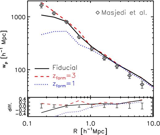
Shown is how the model prediction of the projected correlation function is changed if varying the model parameter in our abundance matching method, in comparison with the SDSS measurement as in Fig. 8. This plot shows the correlation functions from the mock catalogues obtained by changing the formation redshift of LRG-progenitor haloes from zform = 2 (our fiducial choice) to zform = 1 or 3. The different formation redshifts change the prediction mainly at the small scales, in the one-halo regime, because it changes a time duration for each progenitor halo to experience subsequent merging and assembly histories. For example, if changing to zform = 1, the progenitor haloes do not have enough time to experience merger, which decreases a population of satellite LRGs (subhaloes) and in turn leads to the decreased clustering power at the small scales.
The upper panel of Fig. A2 shows how the change of zform alters the HOD as in Fig. 3. As we discussed above, the change to zform = 3 from zform = 2 leads to a smoother HOD shape around the cut-off halo mass for the central LRG HOD extending down to less massive haloes as well as to an increase of satellite LRGs. The choice of zform = 1 leads to opposite effects. On the other hand, the lower panel shows that the projected mass profile of LRG-host haloes is almost unchanged by the change of zform. Thus an accuracy of the mock catalogue can be improved, especially for predicting the small-scale clustering, by further introducing a variation of the formation epochs as additional parameter.
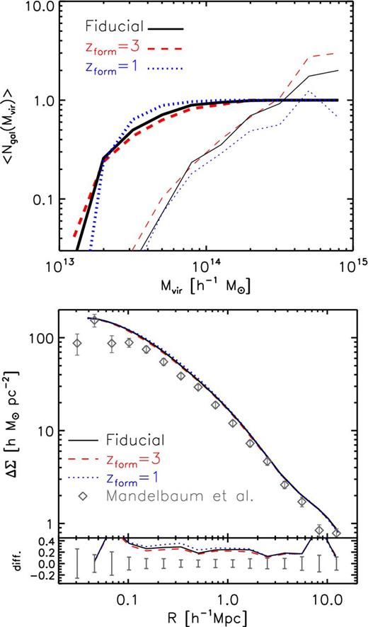
Similarly to the previous plot, but for the HOD (upper panel) and for the projected mass profile (lower panel).
A2 The fraction of LRG-star particles in z = 2 LRG-progenitor halo: fstar
To trace the LRG-progenitor haloes from z = 2 to 0.3, we defined the LRG-star particles in each z = 2 LRG-progenitor halo by the 30 per cent innermost particles of the FoF member particles, fstar = 0.3, assuming that the stars are formed at the central region of each halo. However, the fraction 30 per cent is an arbitrary choice.
Fig. A3 shows how the projected correlation and the HOD are changed by varying to fstar = 0.2 or 0.4 from the fiducial choice of fstar = 0.3. Note that, when matching each z = 2 progenitor halo to a subhalo at z = 0.3, we imposed the condition that a subhalo at z = 0.3 should have more than 50 per cent of the star particles in each of the mock catalogues. Fig. A3 shows that the change of fstar alters the correlation function at the small separation, in the one-halo regime. This is also found from the lower panel, which shows that the change alters the satellite HOD. If we use fstar = 0.4 from 0.3, it tends to include, in the star particles, more loosely bounded member particles in each z = 2 progenitor halo, the star particles tend to be stripped by tidal interaction or merger with other haloes, and then it is in turn difficult to satisfy the 50 per cent matching condition to z = 0.3 subhalo. Thus this results in a smaller number of the survived satellite LRG haloes at z = 0.3, which causes to reduce the correlation amplitude at the small scales. The opposite is true for the case of fstar = 0.2, because it leads to a larger number of the survived satellite LRG haloes at z = 0.3 than in the case of fstar = 0.3. Nevertheless, the encouraging result is the correlation function at large scales in the two-halo regime is not sensitive to the variation of fstar. We have found that the projected mass profile is not changed as in the lower panel of Fig. A2.
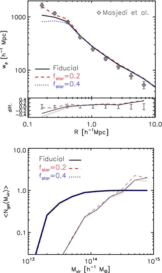
Similarly to the previous figure, but this plot shows the impact of the parameter fstar on the correlation function prediction (upper panel) and on the HOD (lower panel), where fstar is used to define ‘LRG-star’ particles in each LRG-progenitor halo at z = 2 by the fstar fraction of innermost member particles in the halo. Again, changing fstar = 0.2 or 0.4 from our fiducial choice fstar = 0.3 alters the model prediction at the small scales.
A3 The matching fraction between z = 2 LRG-progenitor haloes and z = 0.3 subhaloes: fmatch
Finally, we study how the mock catalogue is changed by varying the matching fraction to fmatch = 0.3 or 0.7 from our fiducial choice fmatch = 0.5. Fig. A4 shows that the change of fmatch alters the projected correlation function at small scales in the one-halo regime and the satellite HOD, similarly to Figs A1 and A3. Again, if increasing the matching fraction to fmatch = 0.7 from 0.5, it leads to a less number of the matched satellite subhaloes at z = 0.3 and in turn leads to a decreased power in the correlation function. On the other hand, the large-scale correlation is more robust to the change of fmatch similarly to the previous figures. We have again found that the projected mass profile is not changed as in the lower panel of Fig. A2.
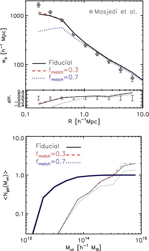
Similarly to the previous figure, but this plot shows the impact of the matching fraction parameter fmatch. In the case of fmatch = 0.5 (our fiducial choice), a subhalo at z = 0.3 is called as LRG-host subhalo if the subhalo contains more than 50 per cent of the star particles in an LRG-progenitor halo at z = 2. The different curves show the results for fmatch = 0.3 or 0.7, which differ from our fiducial model at the small scales.
