Dust and star formation properties of a complete sample of local galaxies drawn from the Planck Early Release Compact Source Catalogue

Clemens, M. S.; Negrello, M.; De Zotti, G.; Gonzalez-Nuevo, J.; Bonavera, L.; Cosco, G.; Guarese, G.; Boaretto, L.; Salucci, P.; Baccigalupi, C.; Clements, D. L.; Danese, L.; Lapi, A.; Mandolesi, N.; Partridge, R.B.; Perrotta, F.; Serjeant, S.; Scott, D.; Toffolatti, L.

doi:10.1093/mnras/stt760

Abstract

We combine Planck High Frequency Instrument data at 857, 545, 353 and 217 GHz with data from Wide-field Infrared Survey Explorer (WISE), Spitzer, IRAS and Herschel to investigate the properties of a well-defined, flux-limited sample of local star-forming galaxies. A 545 GHz flux density limit was chosen so that the sample is 80 per cent complete at this frequency, and the resulting sample contains a total of 234 local, star-forming galaxies. We investigate the dust emission and star formation properties of the sample via various models and calculate the local dust mass function. Although single-component-modified blackbodies fit the dust emission longward of 80 μm very well, with a median β = 1.83, the known degeneracy between dust temperature and β also means that the spectral energy distributions are very well described by a dust component with dust emissivity index fixed at β = 2 and temperature in the range 10–25 K. Although a second, warmer dust component is required to fit shorter wavelength data, and contributes approximately a third of the total infrared emission, its mass is negligible. No evidence is found for a very cold (6–10 K) dust component. The temperature of the cold dust component is strongly influenced by the ratio of the star formation rate to the total dust mass. This implies, contrary to what is often assumed, that a significant fraction of even the emission from ∼20 K dust is powered by ongoing star formation, whether or not the dust itself is associated with star-forming clouds or ‘cirrus’. There is statistical evidence of a free–free contribution to the 217 GHz flux densities of ≲20 per cent. We find a median dust-to-stellar mass ratio of 0.0046; and that this ratio is anticorrelated with galaxy mass. There is good correlation between dust mass and atomic gas mass (median M_d/M_HI = 0.022), suggesting that galaxies that have more dust (higher values of M_d/M_*) have more interstellar medium in general. Our derived dust mass function implies a mean dust mass density of the local Universe (for dust within galaxies), of 7.0 ± 1.4 × 10⁵ M_⊙ Mpc⁻³, significantly greater than that found in the most recent estimate using Herschel data.

galaxies: general, galaxies: luminosity function, mass function, infrared: galaxies, submillimetre: galaxies

INTRODUCTION

The Planck Early Release Compact Source Catalogue (ERCSC) has provided the first complete, all-sky samples of truly local (distances ≲100 Mpc) sub-millimetre selected galaxies. Negrello et al. (2013) have exploited these samples to derive the local luminosity functions at 857, 545, 353 and 217 GHz (350, 550, 850 and 1382 μm). In this paper, we combine Planck/ERCSC data with data from Wide-field Infrared Survey Explorer (WISE), Spitzer, IRAS, Herschel and from optical/near-IR observations to investigate the dust emission and star formation properties using an 80 per cent complete sample selected at 545 GHz (550 μm). We present estimates of the total infrared (IR) luminosity function, of the dust mass function, of the star formation rate (SFR) function, and investigate the distribution of dust temperatures as well as several correlations among the parameters characterizing the dust emission and parameters such as the SFR.

The present sample has a unique combination of properties allowing a robust determination of these quantities that constitute key reference data for evolutionary models. It is drawn from a blind sub-mm survey rather than on follow-up observations of sources selected in other wavebands (e.g. in the optical or in the far-IR). Another important strength is the abundant amount of multifrequency data available for our sources allowing an investigation of the full Spectral Energy Distribution (SED). Moreover, the truly local nature of the sample relieves us from the need of applying evolutionary or k-corrections.

The paper is organized as follows. In Section 2, we describe the sample selection and the auxiliary data used. In Section 3, we present the parameters characterizing the dust emission and the stellar masses obtained using the public code Multiwavelength Analysis of Galaxy Physical Properties (magphys; da Cunha et al. 2008) and discuss their correlations. The distribution functions (dust mass function, IR luminosity function, SFR function) are described in Section 4 and the ensuing global values for the dust mass density, IR luminosity, SFR density in the local universe are given in Section 5. In Section 6, we compare the magphys results with those obtained with simple single- or two-temperature grey body fits. Finally, in Section 7, we summarize our main conclusions.

SAMPLE SELECTION AND AUXILIARY DATA

Negrello et al. (2013) have accurately inspected the ERCSC sources at 857, 545, 353 and 217 GHz in order to identify local star-forming galaxies. We refer the reader to that paper for the details on the source identification process. Here, we use their sample of 234 galaxies with flux density greater than 1.8 Jy at 545 GHz. The authors estimate the sample to be 80 per cent complete. Within this sample, the number of galaxies with flux density measurements at 857, 545, 353 and 217 GHz is 232, 234, 181 and 47, respectively. 232 galaxies have flux densities at 857 and 545 GHz, 181 also have a 353 GHz data and 47 have flux densities at all four frequencies.

All galaxies have redshift-independent distance measurements. These distances, rather than those derived from spectroscopic redshifts, were used in all calculations of masses and luminosities. In fact, for these nearby galaxies, redshifts are poor distance indicators because the contribution of proper motions may be comparable to that of cosmic expansion.

Planck flux densities

The ERCSC offers, for each source, four different flux density measurements (Planck Collaboration VII 2011). Based on the analysis by Negrello et al. (2013), we have adopted the ‘GAUFLUX’ values at 857 and 545 GHz. However, based on a comparison of 353 GHz flux densities with 850 μm flux densities from Submillimetre Common-User Bolometer Array (SCUBA; Dale et al. 2005; Dunne et al. 2000), we use the ‘FLUX’ values at 353 and 217 GHz. As explained in Planck Collaboration (2011), two small corrections need to be applied to the ERCSC flux densities. The first is to take into account that Planck/High Frequency Instrument maps are calibrated to have the correct flux density values for spectra with νI_ν = constant. The colour corrections for spectral indices α ≃ 3 (I_ν ∝ ν^α), as appropriate for our sources, amount to factors: 0.965 (857 GHz), 0.903 (545 GHz), 0.887 (353 GHz) and 0.896 (217 GHz). The second correction is to remove the contribution of the CO emission within the Planck pass-bands; since we are interested in the thermal dust emission, the CO line is a contaminant. The adopted procedure is described in detail in Negrello et al. (2013). The correction factors are 0.978, 0.978 and 0.990 for the 217, 353 and 545 GHz bands, respectively; the correction is negligible at 857 GHz.

Data at other wavelengths

As well as finding optical (U, B, V) flux densities from the RC3 (de Vaucouleurs et al. 1991) and near-IR (J, H, Ks) flux densities from Two Micron All Sky Survey (2MASS) (Jarrett et al. 2003) for all 234 objects, we also cross-correlated our list with catalogues from IR satellites.

IRAS

Matches were sought in both the Faint Source Catalogue (FSC) and Point Source Catalogue (PSC), but the vast majority of matches were found in the FSC. The IRAS flux densities for some larger galaxies, however, are not found in either of these catalogues. Data for these galaxies were taken from either Sanders et al. (2003), Rice et al. (1988), Surace, Sanders & Mazzarella (2004), Soifer et al. (1989) or Lisenfeld et al. (2007). Only four objects (IC 750, NGC 3646, NGC 4145 and NGC 4449) had no IRAS measurements.

AKARI

Both the AKARI-InfraRed Camera PSC (9 and 18 μm) and Bright Source Catalogue (65, 90, 140 and 160 μm) were searched for matches within a 10′′ search radius. Matches with at least one flux density measurement were found for 210/234 objects. However, the AKARI data were found to be, in many cases, inconsistent with IRAS data (typically lower) and not smoothly connected to the photometry in nearby bands. Problems with AKARI photometry were also reported by Serjeant et al. (2012) who found evidence of systematic errors of the order of 30 per cent, of unknown origin but possibly related to sky subtraction, and of saturation for the brightest objects. Yamamura et al. (2010) mention two other possible causes that may contribute to the discrepancies. One is the higher spatial resolution of AKARI that may result in a lower ‘point source’ flux density for our large galaxies. The second is the still large (typically 20 per cent) uncertainty of the AKARI flux calibration. For these reasons, we have not included the AKARI data in our SED fits.

WISE

All but seven of the 234 objects were matched with a search radius of 5′′ in the WISE (Wright et al. 2010) All Sky Data Release. Flux densities at 3.4, 4.6, 12 and 22 μm were taken according to the value of the ‘ext_flag’ parameter. Where |$\rm ext\_flag=5$|⁠, the flux density determined within an aperture defined by the extent of the associated 2MASS source was used (‘w?gmag’¹), otherwise, the flux density determined by standard profile fitting of the source was used (‘w?mpro’). Of the sources for which a match was found, all but four had |$\rm ext\_flag=5$|⁠; however, reliable flux densities could not be determined for 17 galaxies.

Spitzer

Matches were sought from the compilation of Multiband Imaging Photometer for Spitzer (MIPS) data at 24, 70 and 160 μm in Bendo, Galliano & Madden (2012); 32/234 galaxies had flux densities in at least one of the MIPS bands.

Herschel

Four Herschel surveys were searched for matches with the Planck catalogue: the ‘Herschel Reference Survey’ (HRS; Boselli et al. 2010), the ‘Herschel Virgo Cluster Survey’ (HeViCS; Davies et al. 2010), ‘Key Insights on Nearby Galaxies: a Far-IR Survey with Herschel’ (KINGFISH; Kennicutt et al. 2011) and the ‘Herschel–Astrophysical Terahertz Large Area Survey’ (Herschel–ATLAS; Herranz et al. 2013). We found 28 matches with HRS [Ciesla et al. only Spectral and Photometric Imaging Receiver (SPIRE) data; 2012; six with HeViCS [Photodetecting Array Camera and Spectrometer (PACS) 100 and 160 μm + SPIRE data; Davies et al. 2012; 30 with the KINGFISH, most having flux densities at all PACS and SPIRE wavelengths (70, 100, 160, 250, 350 and 500 μm) and three with the Herschel–ATLAS.

A comparison between Planck and Herschel flux densities for overlapping frequency bands is given in Negrello et al. (2013).

FITS TO THE DATA

The public magphys code by da da Cunha et al. (2008) exploits a large library of optical and IR templates linked together in a physically consistent way. It allows us to derive basic physical parameters from multiwavelength photometric data from the UV to the sub-mm. The evolution of the dust-free stellar emission in the magphys library is computed using the population synthesis model of Bruzual & Charlot (2003), by assuming a Chabrier (2003) initial mass function (IMF) that is cut off below 0.1 and above 100 M_⊙; using a Salpeter IMF instead gives stellar masses that are a factor of 1.5 larger.

The attenuation of starlight by dust is described by the two-component model of Charlot & Fall (2000), where dust is associated with the birth clouds (i.e. the dense molecular clouds where stars form) and with the ambient (i.e. diffuse) interstellar medium (ISM). Starlight is assumed to be the only significant heating source (i.e. any contribution from an active galactic nucleus is neglected) and therefore the energy absorbed at UV/optical/near-IR wavelengths exactly equals that re-radiated by dust in the birth clouds and in the diffuse ISM. The dust luminosities contributed by the stellar birth clouds, |$L_{\rm dust}^{\rm BC}$|⁠, and by the ambient ISM, |$L_{\rm dust}^{\rm ISM}$|⁠, are distributed over the wavelength interval 3–1000 μm assuming four main dust components: (i) the emission from polycyclic aromatic hydrocarbons (PAHs); (ii) the mid-IR continuum from small hot grains stochastically heated to temperatures in the range 130–250 K; (iii) the emission from warm dust (30–60 K) in thermal equilibrium; (iv) the emission from cold dust (15–25 K) in thermal equilibrium. The last two components are assumed to be optically thin and are described by modified grey-body template spectra, with fixed values for the dust emissivity index: β = 1.5 for the warm dust and β = 2 for the cold dust, with dust mass absorption coefficient approximated as a power law, such that k_λ ∝ λ^−β with normalization k_850μm = 0.077 m² kg⁻¹ as in Dunne et al. (2000). The choice of the two values of β is based on various studies that suggest that the emissivity index is different in the warm and cold dust components (see da Cunha et al. 2008).

The birth clouds are assumed not to contain any cold dust while the relative contributions to |$L_{\rm dust}^{\rm BC}$| by PAHs, by the hot mid-IR continuum and by the warm dust are kept as adjustable parameters. In the ambient ISM, the contribution to |$L_{\rm dust}^{\rm ISM}$| by cold dust is kept as an adjustable parameter. The relative proportions of the other three components are fixed to the values reproducing the mid-IR cirrus emission of the Milky Way (see da Cunha et al. 2008, for details).

The analysis of the SED of an observed galaxy with magphys is done in two steps. First, a comprehensive library of model SEDs at the same redshift and in the same photometric bands as the observed galaxy is assembled. This library uses 25 000 stellar population models, derived from a wide range of star formation histories, metallicities and dust attenuations, and 50 000 dust emission models obtained from a large range of dust temperatures and fractional contributions of PAHs, hot mid-IR continuum, warm dust and cold dust to the total IR luminosity. The two libraries are linked together by associating to each those SED models that produce a similar value for the fraction of the total dust luminosity contributed by the diffuse ISM. The corresponding SED models are then scaled to the same total dust luminosity. This procedure ensures that the observed SED is modelled in a consistent way from UV to millimetre wavelengths.

Secondly, the χ² goodness of fit is evaluated for each galaxy model in the library² and then the probability density function of any physical parameter is built by weighting the value of that parameter in each model by the probability exp (−χ²/2). The final best estimate of the parameter is the median of the resulting probability density function and the associated confidence interval in the 16th–84th percentile range.

The output of magphys is a large set of parameters including SFRs, stellar masses, effective dust optical depths, dust masses and relative strengths of different dust components. In the following, we will make use of estimates of stellar mass (M_*), dust mass (M_d), cold and warm dust temperatures (T_c and T_w), total (3-1000 μm) IR luminosity of dust emission (L_dust or L_IR), fraction of the IR luminosity due to the cold dust (f_μ = L_c/L_IR) and SFR (averaged over the last 0.1 Gyr).

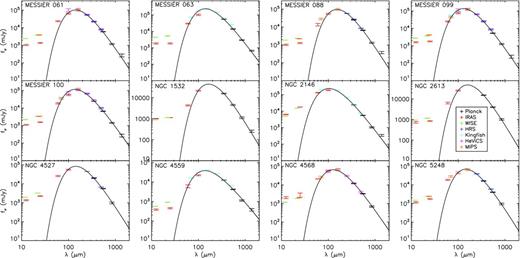
Some example magphys fits for a random sub-set of galaxies in our sample are shown in Fig. 1.

Figure 1.

Open in new tab Download slide

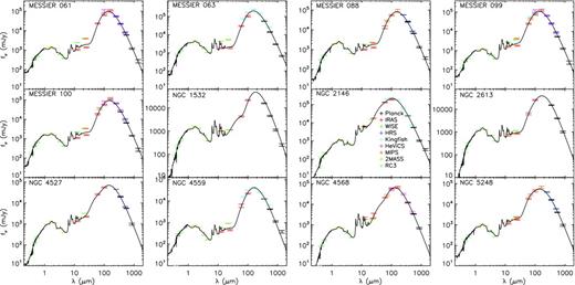
Some example best-fitting SED models produced by magphys.

Dust temperatures and masses

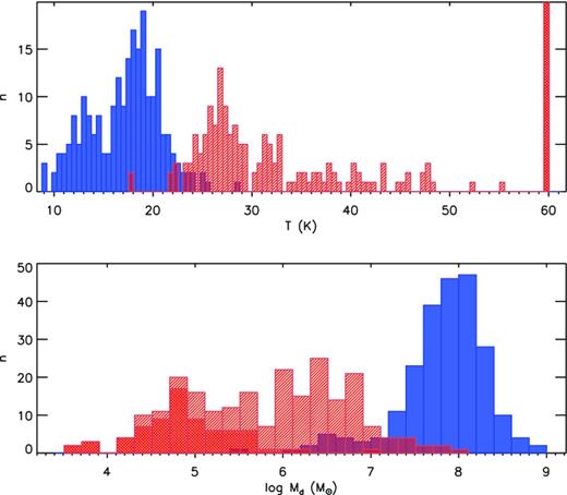
The distributions of the fitted dust temperatures and masses are shown in Fig. 2. The gap between the distributions of the cold and warm dust temperatures is due to the adopted priors. As shown in Section 6, it disappears if the two distributions are allowed to overlap. The median cold dust temperature is 17.7 K. The distribution of warm dust temperatures has a peak in the range 35–38 K and an extended tail towards higher temperatures, raising the median to 43 K.

Figure 2.

Open in new tab Download slide

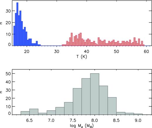
Distributions of temperature and dust mass for magphys fits.

The dust mass in grains in thermal equilibrium at temperature T_d is estimated from their far-IR luminosity L_λ(T_d) using the formula (Hildebrand 1983)

\begin{equation} L_\lambda (T_{\rm d})=4\pi M_{\rm d}(T_{\rm d}) \kappa _\lambda B_\lambda (T_{\rm d}), \end{equation}

(1)

where κ_λ is the dust absorption coefficient and B_λ(T_d) is the blackbody function. The normalization of κ_λ is rather uncertain. magphys adopts κ_850 μm = 0.077 m² kg^{− 1}, as did Dunne et al. (2000). We prefer the more recent value κ_850 μm = 0.0383 m² kg^{− 1} (Draine 2003) because it is derived from a more complete dust model. The earlier value, from Draine & Lee (1984), was derived from a simple ‘graphite–silicate’ model. Therefore, we multiply by a factor of 0.077/0.0383 ≃ 2 the values of M_d given by magphys. Absolute values for dust masses are, in any case, to be used with caution. The median M_d we find in this way is 7.80 × 10⁷ M_⊙.

In Fig. 3, we show how the mass distributions contrast with the total IR luminosity distributions for the cold and warm dust components. Despite the significant contribution of the warm component to the IR luminosity (about 1/3 of the total), the cold component totally dominates the dust mass, with the warm component contributing only ∼1 per cent of the total.

Figure 3.

Open in new tab Download slide

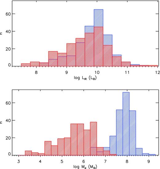
Distributions of the total IR luminosity (3-1000 μm) and dust mass for the warm (red) and cold (blue) dust components of the magphys fits.

Fig. 4 compares the dust masses we obtain using magphys with those estimated by other authors. We see good agreement with the values of Draine et al. (2007) for galaxies in common with the Spitzer Infrared Nearby Galaxy Survey (SINGS). The dust masses estimated by Skibba et al. (2011) for galaxies in the KINGFISH survey are significantly lower than our values (by a factor of ∼3). These authors used single modified blackbody fits with β = 1.5. As discussed in Section 6 and nicely illustrated by Dunne et al. (2000), both of these assumptions tend to underestimate the dust mass. In fact, Skibba et al. (2011) find single-component dust temperatures between 21 and 35 K, so that the lowest value they find is actually warmer than the median value we find for the cool component. This will clearly lead to significantly lower dust masses. Our values are only marginally higher than those found by Auld et al. (2013) in the HeViCS sample, who also used a single-component-modified blackbody fit, but with β = 2.0. Our dust masses are consistent with those found by Planck Collaboration XVI (2011) once the latter are scaled to the same value of κ_d that we have adopted. These masses were determined by scaling the total IR luminosity by constant factors determined by fits to templates.

Figure 4.

Open in new tab Download slide

Comparison of our dust masses with those of other authors. Black: Draine et al. (2007), galaxies with no 850 μm SCUBA flux densities; red: Draine et al. (2007), galaxies with 850 μm flux densities; green: Planck Collaboration XVI (2011); blue: Skibba et al. (2011); cyan: Auld et al. (2013); magenta: Dunne et al. (2000) from two-component fits. Masses have been scaled to a common value of κ_850 μm = 0.0383 m² kg^{− 1} [necessary for Dunne et al. (2000) and Planck Collaboration XVI (2011)].

Dust, atomic gas and stellar mass

The median of the log of the dust to stellar mass ratio is 〈log (M_d/M_*)〉 = −2.34 corresponding to M_d/M_* = 4.6 × 10⁻³. Fig. 5 shows that M_d/M_* is anticorrelated with M_*. The Spearman rank correlation coefficient is −0.68, with the probability of the null hypothesis (no correlation) being 9 × 10⁻³³. The least-squares linear relation between log (M_d/M_*) and log (M_*) is

\begin{equation} {\rm log}\frac{M_{\rm d}}{M_*} = -0.469\,{\rm log} M_* + 2.457. \end{equation}

(2)

We have also checked whether this correlation could be the result of a trend in dust properties with total stellar mass, causing a trend in the value of β that is not modelled. In order to remove this source of doubt, we looked for a correlation between the S₅₄₅/S₃₅₃ ratio (that is a function of β) and the derived stellar mass. No correlation was found, suggesting that there is no bias in the dust mass estimates for different stellar masses and that there is indeed a real anticorrelation between M_d/M_* and M_*.

Figure 5.

Open in new tab Download slide

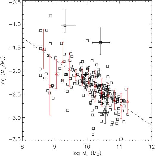
Ratio of dust mass to stellar mass as a function of stellar mass. The error bars are shown on only a small number of points for clarity. The median values in bins of stellar mass are shown in red, where the length of the error bars is the standard deviation within the bin. The dotted line is a least-squares fit to the binned points, excluding the bins with few points.

A similar correlation has also been found by Cortese et al. (2012) based on Herschel data. Lower mass galaxies have higher dust mass fractions than their more massive counterparts. This is perhaps surprising, since the dust-to-gas mass ratio is proportional to the gas metallicity (Draine et al. 2007) and there is a well-established positive correlation between gas-phase metallicity and stellar mass (e.g. Tremonti et al. 2004). On the other hand, the gas-to-stellar mass ratio decreases with stellar mass (Bell & de Jong 2000), and the dust mass also correlates with the gas mass.

To further investigate the dust–gas correlation, we have collected 21 cm H i line fluxes for 225 of our 234 objects from ‘Hyperleda’³ (Paturel et al. 2003). Fluxes were corrected for self-absorption following Heidmann, Heidmann & de Vaucouleurs (1972) with the value of the parameter κ₀ = 0.031, as recommended for spiral galaxies. Atomic gas masses were calculated according to Huchtmeier, Wendker & Tammann (1976):

\begin{equation} \bigg ( \frac{M_{\rm H\,{\small {I}}}}{\mathrm{M}_{{\odot }}}\bigg ) = 2.36\times 10^5 (1+z)^{-1}\,\bigg (\frac{F}{{\rm Jy\,km\,s}^{-1}}\bigg )\;\bigg (\frac{D}{{\rm Mpc}}\bigg )^2. \end{equation}

(3)

For our sample we have set z = 0. Fig. 6 confirms that the total dust and H i masses are well correlated and that the typical galaxy has |$\log (M_{\rm d}/M_{\rm H\,{\small {I}}})=-1.65$| (the dust mass is ≃2.2 per cent of the H i mass). This value is slightly higher than that found by Draine et al. (2007) for the galaxies in common between the SINGS sample and that discussed here. For those galaxies in common, we find |$\langle M_{\rm d}/M_{\rm H\,{\small {I}}}\rangle = 0.013$| for the SINGS observations, and |$\langle M_{\rm d}/M_{\rm H\,{\small {I}}})\rangle = 0.018$| for our work. Draine et al. find mean dust and H i masses of 6.65 × 10⁷ M_⊙ and 5.49 × 10⁹ M_⊙ compared with our values of 6.84 × 10⁷ M_⊙ and 4.03 × 10⁹ M_⊙. Although there is excellent agreement between the dust masses, there is a significant difference in the derived H i masses. This is almost certainly just due to the choice of archival flux measurements made. We chose to the use the average value in Hyperlaeda, where more than one flux measurement was available.

Figure 6.

$Correlation between total dust mass and atomic hydrogen mass. The straight line is for a ratio $M_{\rm d}/M_{\rm H\,{\small {I}}} = 0.02$.$

Open in new tab Download slide

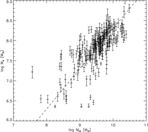
Correlation between total dust mass and atomic hydrogen mass. The straight line is for a ratio |$M_{\rm d}/M_{\rm H\,{\small {I}}} = 0.02$|⁠.

The ratio |$M_{\rm d}/M_{\rm H\,{\small {I}}}$| shows no variation with stellar mass within our sample, so that a plot analogous to Fig. 5 with the H i mass, instead of the dust mass, shows the same trend. Objects with more dust also have more atomic gas. Although we do not have information on the molecular gas content for this sample, it seems clear that objects that are more dusty simply have more ISM, rather than a medium which is richer in dust.⁴ We must therefore conclude that lower mass galaxies have proportionally more dust because they have proportionally more ISM and this effect dominates despite the tendency for lower mass galaxies to be of lower metallicity.

Dust mass versus SFR

It is currently still unknown whether the net effect of a burst of star formation is to increase or decrease the mass of dust within a galaxy. Both production mechanisms [asymptotic giant branch (AGB) stars and perhaps supernovae] and destruction mechanisms (supernova shocks and hot gas) would increase during a star formation episode with differing temporal profiles. With this in mind we now look at the SFR as a function of various derived parameters.

In Fig. 7, we plot the dust mass per unit stellar mass against the SFR. The two quantities are correlated (Spearman's rank correlation coefficient of 0.38 with a chance probability of 3 × 10⁻⁹). A similar result was reported by da Cunha et al. (2010). The least-squares linear relation is log (M_d/M_*) = 0.257 log (SFR)-2.36, and we have checked that, for galaxies in our sample, there is no significant correlation between SFR and M_* (Spearman's rank correlation coefficient of 0.08). Therefore, the SFR correlates with dust mass. This is confirmed by Kendall's partial rank correlation coefficient which indicates that log (M_d) is correlated with the SFR independent of any correlation of each with M_* (correlation coefficient 0.37 with a vanishing probability of chance occurrence). The lack of correlation with stellar mass may be surprising given that several works do find a correlation both in the local Universe (e.g. Brinchmann et al. 2004) and at intermediate and high redshift (e.g. González et al. 2010). The reason for this is probably simply that we do not sample a large enough range of stellar mass (all our objects lie in an interval of three orders of magnitude, and most of these between 10⁹ and 10¹¹ M_⊙ with a median value of 1.8 × 10¹⁰ M_⊙), and that the sample size is insufficient to reveal the correlation, that indeed has a very large scatter. Over the stellar mass range that we sample, the dust mass of a galaxy is more important in determining the SFR than is the total stellar mass.

Figure 7.

Open in new tab Download slide

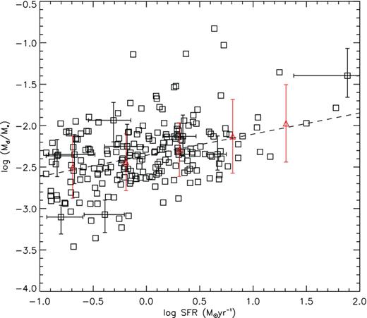
Dust mass per unit stellar mass as a function of the SFR. The dashed line is the least-square fit. The error bars are shown on only a small number of points for clarity. The red symbols indicate the median and standard deviation in bins of SFR.

The observation that the SFR is correlated with the dust mass is not surprising given that a higher dust mass implies a larger ISM mass in general, as we saw in Section 3.2. That the ISM surface density determines the SFR has long been known (see, e.g. Kennicutt 1998).

SFR versus dust temperature

Fig. 8 (top) compares the SFR per unit dust mass (SFR/M_d) with the cold dust temperature, T_c. There is a highly significant correlation (Spearman's rank correlation coefficient of 0.56 with a chance probability of 10⁻¹⁹) especially for T_c ≳ 18 K. The least-squares linear correlation is given by log(SFR/M_d) = 0.167 T_c − 10.9. Again, the Kendall partial rank correlation coefficient (0.42 with a vanishing chance probability) shows that the correlation is not due to a correlation between either the dust temperature or SFR and the dust mass. There is therefore a physical link between the SFR per unit dust mass and T_c. Interestingly, Lagache et al. (1998) find that, in the Milky Way, the equilibrium dust temperature of the diffuse ‘cirrus’ is about 17.5 K, with only small variations over the high Galactic latitude sky.

Figure 8.

$Top: SFR per unit dust mass as a function of the cold dust temperature. The dashed line is the least-squares linear relation. The red symbols indicate the median and the standard deviation in bins of temperature. Bottom: SFR surface density, estimated as the $\rm SFR/D_{25}^2$, as a function of the cold dust temperature. Only a few representative error bars are shown for each plot.$

Open in new tab Download slide

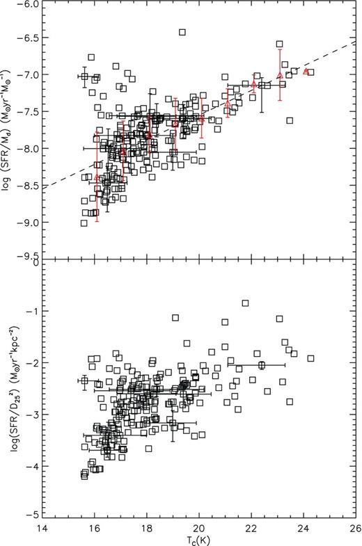
Top: SFR per unit dust mass as a function of the cold dust temperature. The dashed line is the least-squares linear relation. The red symbols indicate the median and the standard deviation in bins of temperature. Bottom: SFR surface density, estimated as the |$\rm SFR/D_{25}^2$|⁠, as a function of the cold dust temperature. Only a few representative error bars are shown for each plot.

In interpreting this correlation, it is useful to consider two ideal cases. If cold dust emission arises from high filling factor regions of low optical depth (cirrus) where the dust temperature is defined by the intensity of the interstellar radiation field (ISRF), as assumed by da Cunha et al. (2008), then T_c would be independent of the SFR and no correlation would be seen in Fig. 8. On the other hand, if the cold dust emission were heated by young stars in star-forming regions only, then the SFR would be directly given by the far-IR luminosity, |$L_{\text{FIR}}$| and, by equation (1), we would find |$\hbox{SFR}/M_{\rm d} \propto T_{\rm c}^{4+\beta }$|⁠. Physically, this describes internally heated clouds where optical and UV photons (to which the clouds are optically thick) are absorbed close to the internal heating source and the bulk of the cloud is then heated by the secondary IR radiation emitted by the more internal dust (Whittet 1992). The dust temperature is defined by the internal heating luminosity, which is proportional to the SFR in the case of a region of star formation. In this case, an increase in the SFR for fixed dust mass will result in an increase in the dust temperature (and likewise a decrease in dust mass for a given SFR).

We see in Fig. 8 that for T_c ≲ 18 K the correlation is weaker, as would be expected if dust heating by the passive stellar population were important. At higher temperatures the correlation is stronger, implying an important role of star formation in heating the cold dust. When the dust is warmer it is heated more by ongoing star formation.

However, having established that ongoing star formation plays an important role in heating the cold dust component, it may not necessarily be the case that the dust emission itself (or even a part thereof) actually comes from dust in the star-forming clouds. Many star-forming regions are quite visible in the optical, and so a lower dust mass may imply a less complete shield against internally generated UV photons and so more may escape to the general ISM. In this case, the lower dust mass in the star-forming clouds would increase the general ISRF and therefore the temperature of the cirrus emission. Whatever the geometrical situation (dust emission from star-forming clouds or cirrus heated by UV photons escaping from the same), the conclusion remains that star-forming regions play a role in defining the temperature of the cold dust component, especially for sources with cold dust temperatures over 18 K.

The relationship between the ISRF and dust temperature can be investigated via the optical radii of the galaxies as given in the RC3 (de Vaucouleurs et al. 1991). In the lower panel of Fig. 8, we plot the SFR divided by the square of the optical major isophotal diameter, D₂₅, at the surface brightness level μ_B = 25 Bmag/arcsec² (which provides a crude estimate of the ISRF due to star formation). A correlation is seen also in this case, though less strong than that in the top panel, consistent with a picture in which star formation contributes to the cirrus dust heating by increasing the general ISRF. However, the correlation is not seen if we replace the SFR with the total stellar mass in the lower panel of Fig. 8. As this is a crude estimate of the stellar surface density, objects with higher stellar surface density should have a higher ISRF contribution from the quiescent stellar population. The lack of a correlation in this case would be surprising if the quiescent population were the main driver of T_c.

Though these correlations should not be overinterpreted, taken together, they strongly indicate that the ∼20 K dust emission in our sample of galaxies has a very significant energy input from ongoing star formation, whether or not the dust itself is associated with star-forming clouds or ‘cirrus’.

No correlations are found with the warm dust temperature,⁵ though we note that these temperatures are less well constrained. This is consistent with the finding by Lapi et al. (2011) that star formation regions have quite uniform dust temperatures.

It is important to view the link between SFR and T_c in the context of previous results and underline how it extends what has been known since IRAS times. A tendency for galaxies with higher specific SFRs (measured as L_IR/L_B) to have warmer S₁₀₀/S₆₀ colours (de Jong et al. 1984) and also an anticorrelation between S₆₀/S₁₀₀ and S₁₂/S₂₅ (Helou 1986) led to the two-component model of dust emission in galaxies. In this model, warm (∼50 K) dust is associated with regions of star formation and relatively cool (∼25 K) dust is associated with, and heated by, the passive stellar population. This latter component is often referred to as ‘cirrus’. Galaxies with higher specific SFRs have a larger fraction of warm dust and their IRAS colours reflect this.

What we find refers only to the cold component in this picture. We argue that this component is also heated significantly by star formation. Not only does the specific SFR change the fraction of cold to warm dust as found by previous studies, but the ratio of SFR to dust mass affects the temperature of the cold component.

SFR versus L_IR

Both the far-IR (40-500 μm) luminosity, L_FIR, and the total (8-1000 μm) IR luminosity, L_IR, are commonly used to estimate the SFR using relations such as (Kennicutt & Evans 2012)

\begin{equation} {\rm SFR}/{\rm M_{{\odot }}\,yr^{-1}} = 1.5 \times 10^{-10}\, L_{\rm IR}/\mathrm{L}_{{\odot }}. \end{equation}

(4)

However, as can be seen in Fig. 3, the contribution to the total IR luminosity of the cold dust (typically assumed to be cirrus heated by the general ISRF – but see above) can be similar to that of the warm dust (presumably heated by young stars). In Fig. 3, the cold component is approximately twice as luminous as the warm component.

Fig. 9 explores this issue by comparing the star formation derived using equation (4) for both the total IR luminosity and the IR luminosity of just the warm dust component. Also shown are the SFRs output by magphys. At high L_IR the total IR luminosity is a good proxy for the SFR. However for L_IR ≲ 5 × 10⁹ L_⊙ this is really no longer true. In some objects the IR emission of the warm dust would give a good estimate of the SFR, but in other, less extincted objects, the optical/UV emission would also need to be taken into consideration (red points above the solid line in Fig. 9). The dashed line in Fig. 9 is given by

\begin{eqnarray} \log ({\rm SFR}/{\rm M}_{{\odot }}\,\mathrm{yr}^{-1})& =& -9.6 + \log (L_{\rm IR}/\mathrm{L}_{\odot })\nonumber\\ && - \,\bigg (\frac{2.0}{\log (L_{\rm IR}/\mathrm{L}_{\odot }) -7.0}\bigg ) \end{eqnarray}

(5)

and can be used to derive SFRs from L_IR when no other information is available.

Figure 9.

Open in new tab Download slide

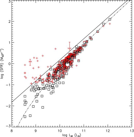
SFR as a function of the total IR luminosity, L_IR (3-1000 μm). The black squares are the SFR that would be obtained by using the IR luminosity of the warm dust component in equation (4), whereas the solid black line shows the SFR that would be obtained by using the total IR luminosity in equation (4). The red symbols are the SFR as derived by magphys.

DISTRIBUTION FUNCTIONS

Dust mass function

The dust mass function is estimated from the 545 GHz local luminosity function produced by Negrello et al. (2013, their table 5), which is based on the same flux-limited sample analysed here and is already corrected for incompleteness. However, because dust temperatures vary, we cannot directly transform the 545 GHz luminosity into a dust mass. We therefore calculate the mass function by considering the distribution of dust masses within bins of 545 GHz luminosity. For each logarithmic bin of luminosity the number of galaxies in each logarithmic mass bin is calculated, giving the mass function within a restricted range of luminosities. The mass function within each bin of luminosity is then multiplied by the appropriate value of the luminosity function ( number in the rightmost column in Table 1) to obtain the contribution of that luminosity bin to the total function. The total dust mass function is then given by the summation of the contributions in a given mass bin (vertical summation in Table 1). Table 1 lists the number of objects in each individual bin.

Table 1.

The number of objects in each logarithmic bin of dust mass (in solar units) and monochromatic luminosity (in W/Hz) for the mass function derived from magphys dust masses. The last column contains the log of the 545 GHz luminosity function by Negrello et al. (2013) while the last row contains the log of the derived dust mass function. Both the luminosity and the mass function are in Mpc⁻³ dex⁻¹.

log (M_d)	6.4	6.7	7.0	7.3	7.6	7.9	8.2	8.5	8.8	9.1	LF
log (L₅₄₅)
21.63	2	1	0	0	0	0	0	0	0	0	\|$-1.29^{+0.18}_{-0.31}$\|
21.93	0	6	3	0	0	0	0	0	0	0	\|$-1.47^{+0.14}_{-0.20}$\|
22.23	0	0	4	8	0	0	0	0	0	0	\|$-1.73^{+0.12}_{-0.16}$\|
22.53	0	0	0	7	11	0	0	0	0	0	\|$-1.95^{+0.08}_{-0.10}$\|
22.83	0	0	0	0	26	19	1	0	0	0	\|$-2.02^{+0.06}_{-0.06}$\|
23.13	0	0	0	0	2	46	35	0	0	0	\|$-2.32^{+0.05}_{-0.06}$\|
23.43	0	0	0	0	0	0	28	15	0	0	\|$-2.86^{+0.06}_{-0.06}$\|
23.73	0	0	0	0	0	0	1	9	1	0	\|$-3.68^{+0.09}_{-0.11}$\|
24.03	0	0	0	0	0	0	0	0	2	0	\|$-4.60^{+0.14}_{-0.20}$\|
24.33	0	0	0	0	0	0	0	0	0	1	\|$-5.74^{+0.27}_{-0.92}$\|
	\|$-1.27^{+0.38}_{-0.73}$\|	\|$-1.70^{+0.32}_{-0.32}$\|	\|$-1.70^{+0.24}_{-0.28}$\|	\|$-1.83^{+0.16}_{-0.19}$\|	\|$-1.92^{+0.11}_{-0.11}$\|	\|$-2.22^{+0.08}_{-0.08}$\|	\|$-2.68^{+0.09}_{-0.07}$\|	\|$-3.46^{+0.11}_{-0.12}$\|	\|$-4.61^{+0.36}_{-0.36}$\|	−5.75^+0.54

log (M_d)	6.4	6.7	7.0	7.3	7.6	7.9	8.2	8.5	8.8	9.1	LF
log (L₅₄₅)
21.63	2	1	0	0	0	0	0	0	0	0	\|$-1.29^{+0.18}_{-0.31}$\|
21.93	0	6	3	0	0	0	0	0	0	0	\|$-1.47^{+0.14}_{-0.20}$\|
22.23	0	0	4	8	0	0	0	0	0	0	\|$-1.73^{+0.12}_{-0.16}$\|
22.53	0	0	0	7	11	0	0	0	0	0	\|$-1.95^{+0.08}_{-0.10}$\|
22.83	0	0	0	0	26	19	1	0	0	0	\|$-2.02^{+0.06}_{-0.06}$\|
23.13	0	0	0	0	2	46	35	0	0	0	\|$-2.32^{+0.05}_{-0.06}$\|
23.43	0	0	0	0	0	0	28	15	0	0	\|$-2.86^{+0.06}_{-0.06}$\|
23.73	0	0	0	0	0	0	1	9	1	0	\|$-3.68^{+0.09}_{-0.11}$\|
24.03	0	0	0	0	0	0	0	0	2	0	\|$-4.60^{+0.14}_{-0.20}$\|
24.33	0	0	0	0	0	0	0	0	0	1	\|$-5.74^{+0.27}_{-0.92}$\|
	\|$-1.27^{+0.38}_{-0.73}$\|	\|$-1.70^{+0.32}_{-0.32}$\|	\|$-1.70^{+0.24}_{-0.28}$\|	\|$-1.83^{+0.16}_{-0.19}$\|	\|$-1.92^{+0.11}_{-0.11}$\|	\|$-2.22^{+0.08}_{-0.08}$\|	\|$-2.68^{+0.09}_{-0.07}$\|	\|$-3.46^{+0.11}_{-0.12}$\|	\|$-4.61^{+0.36}_{-0.36}$\|	−5.75^+0.54

Open in new tab

Table 1.

The number of objects in each logarithmic bin of dust mass (in solar units) and monochromatic luminosity (in W/Hz) for the mass function derived from magphys dust masses. The last column contains the log of the 545 GHz luminosity function by Negrello et al. (2013) while the last row contains the log of the derived dust mass function. Both the luminosity and the mass function are in Mpc⁻³ dex⁻¹.

log (M_d)	6.4	6.7	7.0	7.3	7.6	7.9	8.2	8.5	8.8	9.1	LF
log (L₅₄₅)
21.63	2	1	0	0	0	0	0	0	0	0	\|$-1.29^{+0.18}_{-0.31}$\|
21.93	0	6	3	0	0	0	0	0	0	0	\|$-1.47^{+0.14}_{-0.20}$\|
22.23	0	0	4	8	0	0	0	0	0	0	\|$-1.73^{+0.12}_{-0.16}$\|
22.53	0	0	0	7	11	0	0	0	0	0	\|$-1.95^{+0.08}_{-0.10}$\|
22.83	0	0	0	0	26	19	1	0	0	0	\|$-2.02^{+0.06}_{-0.06}$\|
23.13	0	0	0	0	2	46	35	0	0	0	\|$-2.32^{+0.05}_{-0.06}$\|
23.43	0	0	0	0	0	0	28	15	0	0	\|$-2.86^{+0.06}_{-0.06}$\|
23.73	0	0	0	0	0	0	1	9	1	0	\|$-3.68^{+0.09}_{-0.11}$\|
24.03	0	0	0	0	0	0	0	0	2	0	\|$-4.60^{+0.14}_{-0.20}$\|
24.33	0	0	0	0	0	0	0	0	0	1	\|$-5.74^{+0.27}_{-0.92}$\|
	\|$-1.27^{+0.38}_{-0.73}$\|	\|$-1.70^{+0.32}_{-0.32}$\|	\|$-1.70^{+0.24}_{-0.28}$\|	\|$-1.83^{+0.16}_{-0.19}$\|	\|$-1.92^{+0.11}_{-0.11}$\|	\|$-2.22^{+0.08}_{-0.08}$\|	\|$-2.68^{+0.09}_{-0.07}$\|	\|$-3.46^{+0.11}_{-0.12}$\|	\|$-4.61^{+0.36}_{-0.36}$\|	−5.75^+0.54

log (M_d)	6.4	6.7	7.0	7.3	7.6	7.9	8.2	8.5	8.8	9.1	LF
log (L₅₄₅)
21.63	2	1	0	0	0	0	0	0	0	0	\|$-1.29^{+0.18}_{-0.31}$\|
21.93	0	6	3	0	0	0	0	0	0	0	\|$-1.47^{+0.14}_{-0.20}$\|
22.23	0	0	4	8	0	0	0	0	0	0	\|$-1.73^{+0.12}_{-0.16}$\|
22.53	0	0	0	7	11	0	0	0	0	0	\|$-1.95^{+0.08}_{-0.10}$\|
22.83	0	0	0	0	26	19	1	0	0	0	\|$-2.02^{+0.06}_{-0.06}$\|
23.13	0	0	0	0	2	46	35	0	0	0	\|$-2.32^{+0.05}_{-0.06}$\|
23.43	0	0	0	0	0	0	28	15	0	0	\|$-2.86^{+0.06}_{-0.06}$\|
23.73	0	0	0	0	0	0	1	9	1	0	\|$-3.68^{+0.09}_{-0.11}$\|
24.03	0	0	0	0	0	0	0	0	2	0	\|$-4.60^{+0.14}_{-0.20}$\|
24.33	0	0	0	0	0	0	0	0	0	1	\|$-5.74^{+0.27}_{-0.92}$\|
	\|$-1.27^{+0.38}_{-0.73}$\|	\|$-1.70^{+0.32}_{-0.32}$\|	\|$-1.70^{+0.24}_{-0.28}$\|	\|$-1.83^{+0.16}_{-0.19}$\|	\|$-1.92^{+0.11}_{-0.11}$\|	\|$-2.22^{+0.08}_{-0.08}$\|	\|$-2.68^{+0.09}_{-0.07}$\|	\|$-3.46^{+0.11}_{-0.12}$\|	\|$-4.61^{+0.36}_{-0.36}$\|	−5.75^+0.54

Open in new tab

Fig. 10 shows the dust mass function that results using the magphys-derived dust masses, scaled to the value of κ_d given by Draine (2003, see Section 3.1) and the best-fitting Schechter function:

\begin{equation} \Phi _d(M)\text{d}M = \phi _d^*\,\Big (\frac{M}{M_{\rm d}^*}\Big )^{\alpha _d}\,\text{e}^{-(M/M_{\rm d}^*)}\,\frac{\text{d}M}{M_{\rm d}^*}. \end{equation}

(6)

The best-fitting values of the parameters |$\phi _d^*$|⁠, |$M_{\rm d}^*$| and α_d are given in Table 2.

Figure 10.

Open in new tab Download slide

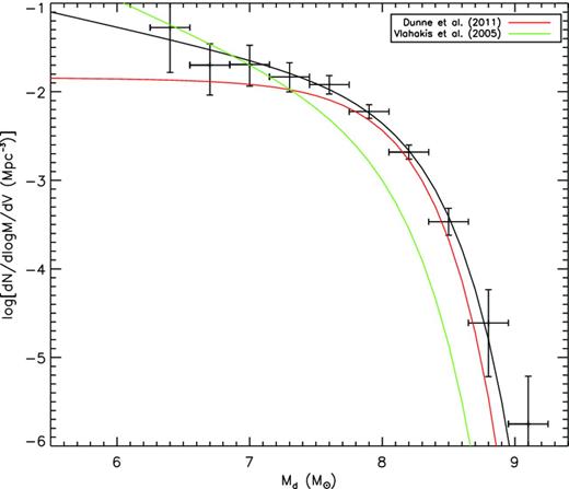
Dust mass function calculated from the luminosity function at 545 GHz as presented in Negrello et al. (2013) and the magphys-derived dust masses. The black line shows the best-fitting Schechter function with parameters given in Table 2. The red and green lines show the dust mass functions of Dunne et al. (2011) and Vlahakis et al. (2005) after scaling them to approximately account for the different value of κ_d used by these authors.

Table 2.

Schechter fit parameters for dust masses derived with various models and different values of the dust mass absorption coefficient, κ_d. Our favoured model is shown in bold face.

Model	α_d	\|$M_{\rm d}^*$\|	\|$\phi _d^*$\|
		(M_⊙)	(Mpc^{− 3} dex^{− 1})
Single-temperature grey body	−1.30 ± 0.27	1.13 ± 0.46 × 10⁸	3.00 ± 1.96 × 10⁻³
Two-temperature grey bodies	−1.42 ± 0.39	1.43 ± 0.63 × 10⁸	4.49 ± 3.62 × 10⁻³
MAGPHYS	−1.34 ± 0.36	1.06 ± 0.49 × 10⁸	4.78 ± 3.38 × 10⁻³
Single-temperature grey body*	−1.29 ± 0.33	4.42 ± 2.08 × 10⁷	3.30 ± 2.42 × 10⁻³
Two-temperature grey bodies*	−1.45 ± 0.40	6.00 ± 2.51 × 10⁷	4.42 ± 3.52 × 10⁻³
MAGPHYS*	−1.34 ± 0.36	5.32 ± 2.01 × 10⁷	4.77 ± 3.10 × 10⁻³
Dunne et al. (2011)*	−1.01	3.83 × 10⁷	5.87 × 10⁻³
Vlahakis, Dunne & Eales (2005)*	−1.67	3.09 × 10⁷	3.01 × 10⁻³

Model	α_d	\|$M_{\rm d}^*$\|	\|$\phi _d^*$\|
		(M_⊙)	(Mpc^{− 3} dex^{− 1})
Single-temperature grey body	−1.30 ± 0.27	1.13 ± 0.46 × 10⁸	3.00 ± 1.96 × 10⁻³
Two-temperature grey bodies	−1.42 ± 0.39	1.43 ± 0.63 × 10⁸	4.49 ± 3.62 × 10⁻³
MAGPHYS	−1.34 ± 0.36	1.06 ± 0.49 × 10⁸	4.78 ± 3.38 × 10⁻³
Single-temperature grey body*	−1.29 ± 0.33	4.42 ± 2.08 × 10⁷	3.30 ± 2.42 × 10⁻³
Two-temperature grey bodies*	−1.45 ± 0.40	6.00 ± 2.51 × 10⁷	4.42 ± 3.52 × 10⁻³
MAGPHYS*	−1.34 ± 0.36	5.32 ± 2.01 × 10⁷	4.77 ± 3.10 × 10⁻³
Dunne et al. (2011)*	−1.01	3.83 × 10⁷	5.87 × 10⁻³
Vlahakis, Dunne & Eales (2005)*	−1.67	3.09 × 10⁷	3.01 × 10⁻³

*Computed with a coefficient κ_d a factor of ≃2 higher, yielding dust masses a factor of ≃2 lower, see Section 3.1.

Open in new tab

Table 2.

Schechter fit parameters for dust masses derived with various models and different values of the dust mass absorption coefficient, κ_d. Our favoured model is shown in bold face.

Model	α_d	\|$M_{\rm d}^*$\|	\|$\phi _d^*$\|
		(M_⊙)	(Mpc^{− 3} dex^{− 1})
Single-temperature grey body	−1.30 ± 0.27	1.13 ± 0.46 × 10⁸	3.00 ± 1.96 × 10⁻³
Two-temperature grey bodies	−1.42 ± 0.39	1.43 ± 0.63 × 10⁸	4.49 ± 3.62 × 10⁻³
MAGPHYS	−1.34 ± 0.36	1.06 ± 0.49 × 10⁸	4.78 ± 3.38 × 10⁻³
Single-temperature grey body*	−1.29 ± 0.33	4.42 ± 2.08 × 10⁷	3.30 ± 2.42 × 10⁻³
Two-temperature grey bodies*	−1.45 ± 0.40	6.00 ± 2.51 × 10⁷	4.42 ± 3.52 × 10⁻³
MAGPHYS*	−1.34 ± 0.36	5.32 ± 2.01 × 10⁷	4.77 ± 3.10 × 10⁻³
Dunne et al. (2011)*	−1.01	3.83 × 10⁷	5.87 × 10⁻³
Vlahakis, Dunne & Eales (2005)*	−1.67	3.09 × 10⁷	3.01 × 10⁻³

Model	α_d	\|$M_{\rm d}^*$\|	\|$\phi _d^*$\|
		(M_⊙)	(Mpc^{− 3} dex^{− 1})
Single-temperature grey body	−1.30 ± 0.27	1.13 ± 0.46 × 10⁸	3.00 ± 1.96 × 10⁻³
Two-temperature grey bodies	−1.42 ± 0.39	1.43 ± 0.63 × 10⁸	4.49 ± 3.62 × 10⁻³
MAGPHYS	−1.34 ± 0.36	1.06 ± 0.49 × 10⁸	4.78 ± 3.38 × 10⁻³
Single-temperature grey body*	−1.29 ± 0.33	4.42 ± 2.08 × 10⁷	3.30 ± 2.42 × 10⁻³
Two-temperature grey bodies*	−1.45 ± 0.40	6.00 ± 2.51 × 10⁷	4.42 ± 3.52 × 10⁻³
MAGPHYS*	−1.34 ± 0.36	5.32 ± 2.01 × 10⁷	4.77 ± 3.10 × 10⁻³
Dunne et al. (2011)*	−1.01	3.83 × 10⁷	5.87 × 10⁻³
Vlahakis, Dunne & Eales (2005)*	−1.67	3.09 × 10⁷	3.01 × 10⁻³

*Computed with a coefficient κ_d a factor of ≃2 higher, yielding dust masses a factor of ≃2 lower, see Section 3.1.

Open in new tab

Also shown in Fig. 10 are the best-fitting Schechter functions from Dunne et al. (2011) and Vlahakis et al. (2005), after scaling them to approximately account for the different value of the dust mass opacity coefficient, κ_d, used by these authors. The value of κ_d we adopted (from Draine 2003, see Section 3.1) is about a factor of 2 lower (implying dust masses about a factor of 2 higher) than that assumed in these two works. With this modification, the agreement between our dust mass function and those of the other two works is good. We find a mass function similar to Vlahakis et al. (2005) below 10⁷ M_⊙ and similar to Dunne et al. (2011) above 10⁷ M_⊙, so that our function is always close to the maximum value of either of the previous determinations. Interestingly, the present sample has detected similar numbers of low dust mass systems to the optically selected sample of Vlahakis et al. (2005).

Total infrared luminosity function

Having well-constrained model fits over the whole IR wavelength range, we can also calculate the total IR luminosities, L_IR, and the corresponding total IR luminosity function. Because there is not a one-to-one relation between a given 545 GHz luminosity and the corresponding total far-IR luminosity, we use the same bivariate method applied above to calculate the dust mass function, based on the 545 GHz luminosity function. This total IR luminosity function is shown in Fig. 11, and the corresponding data tabulated in Table 3.

Figure 11.

$Total far-IR (3–1000 μm) luminosity function calculated from the luminosity function at 545 GHz as presented in Negrello et al. (2013) and the magphys-derived far-IR luminosities. The black line shows the best-fitting Schechter function with parameters, α = −1.78 ± 0.18, $L_{\rm IR}^* = 1.71 \times 10^{11}\,\mathrm{L}_{\odot }$ and ϕ* = 3.60 ± 1.72 × 10−4 Mpc−3 dex−1. The red symbols show the same luminosity function calculated using just the IRAS 60 and 100 μm flux densities and the green symbols show the luminosity function as derived by Sanders et al. (2003).$

Open in new tab Download slide

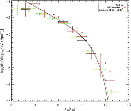
Total far-IR (3–1000 μm) luminosity function calculated from the luminosity function at 545 GHz as presented in Negrello et al. (2013) and the magphys-derived far-IR luminosities. The black line shows the best-fitting Schechter function with parameters, α = −1.78 ± 0.18, |$L_{\rm IR}^* = 1.71 \times 10^{11}\,\mathrm{L}_{\odot }$| and ϕ* = 3.60 ± 1.72 × 10⁻⁴ Mpc⁻³ dex⁻¹. The red symbols show the same luminosity function calculated using just the IRAS 60 and 100 μm flux densities and the green symbols show the luminosity function as derived by Sanders et al. (2003).

Table 3.

The number of objects in each logarithmic bin of total far-IR luminosity (in solar units) and monochromatic 545 GHz luminosity (in W/Hz) for the magphys derived far-IR luminosities. The last column contains the log of the 545 GHz luminosity function by Negrello et al. (2013) while the last row contains the log of the derived IR luminosity function, both in Mpc⁻³ dex⁻¹.

log (L_IR)	8.6	9.0	9.4	9.8	10.2	10.6	11.0	11.4	11.8	12.2	LF
log (L₅₄₅)
21.63	1	2	0	0	0	0	0	0	0	0	\|$-1.29^{+0.18}_{-0.31}$\|
21.93	3	5	1	0	0	0	0	0	0	0	\|$-1.47^{+0.14}_{-0.20}$\|
22.23	1	9	1	1	0	0	0	0	0	0	\|$-1.73^{+0.12}_{-0.16}$\|
22.53	0	0	14	4	0	0	0	0	0	0	\|$-1.95^{+0.08}_{-0.10}$\|
22.83	0	0	7	26	11	2	0	0	0	0	\|$-2.02^{+0.06}_{-0.06}$\|
23.13	0	0	0	12	51	17	3	0	0	0	\|$-2.32^{+0.05}_{-0.06}$\|
23.43	0	0	0	2	10	27	3	1	0	0	\|$-2.86^{+0.06}_{-0.06}$\|
23.73	0	0	0	0	0	1	7	2	1	0	\|$-3.68^{+0.09}_{-0.11}$\|
24.03	0	0	0	0	0	0	2	0	0	0	\|$-4.60^{+0.14}_{-0.20}$\|
24.33	0	0	0	0	0	0	0	0	0	1	\|$-5.74^{+0.27}_{-0.92}$\|
	\|$-1.54^{+0.38}_{-0.40}$\|	\|$-1.19^{+0.24}_{-0.26}$\|	\|$-1.81^{+0.22}_{-0.16}$\|	\|$-1.99^{+0.16}_{-0.11}$\|	\|$-2.25^{+0.08}_{-0.08}$\|	\|$-2.64^{+0.11}_{-0.09}$\|	\|$-3.37^{+0.18}_{-0.15}$\|	\|$-4.16^{+0.36}_{-0.33}$\|	\|$-4.72^{+0.52}_{-0.84}$\|	−5.75^+0.54

log (L_IR)	8.6	9.0	9.4	9.8	10.2	10.6	11.0	11.4	11.8	12.2	LF
log (L₅₄₅)
21.63	1	2	0	0	0	0	0	0	0	0	\|$-1.29^{+0.18}_{-0.31}$\|
21.93	3	5	1	0	0	0	0	0	0	0	\|$-1.47^{+0.14}_{-0.20}$\|
22.23	1	9	1	1	0	0	0	0	0	0	\|$-1.73^{+0.12}_{-0.16}$\|
22.53	0	0	14	4	0	0	0	0	0	0	\|$-1.95^{+0.08}_{-0.10}$\|
22.83	0	0	7	26	11	2	0	0	0	0	\|$-2.02^{+0.06}_{-0.06}$\|
23.13	0	0	0	12	51	17	3	0	0	0	\|$-2.32^{+0.05}_{-0.06}$\|
23.43	0	0	0	2	10	27	3	1	0	0	\|$-2.86^{+0.06}_{-0.06}$\|
23.73	0	0	0	0	0	1	7	2	1	0	\|$-3.68^{+0.09}_{-0.11}$\|
24.03	0	0	0	0	0	0	2	0	0	0	\|$-4.60^{+0.14}_{-0.20}$\|
24.33	0	0	0	0	0	0	0	0	0	1	\|$-5.74^{+0.27}_{-0.92}$\|
	\|$-1.54^{+0.38}_{-0.40}$\|	\|$-1.19^{+0.24}_{-0.26}$\|	\|$-1.81^{+0.22}_{-0.16}$\|	\|$-1.99^{+0.16}_{-0.11}$\|	\|$-2.25^{+0.08}_{-0.08}$\|	\|$-2.64^{+0.11}_{-0.09}$\|	\|$-3.37^{+0.18}_{-0.15}$\|	\|$-4.16^{+0.36}_{-0.33}$\|	\|$-4.72^{+0.52}_{-0.84}$\|	−5.75^+0.54

Open in new tab

Table 3.

The number of objects in each logarithmic bin of total far-IR luminosity (in solar units) and monochromatic 545 GHz luminosity (in W/Hz) for the magphys derived far-IR luminosities. The last column contains the log of the 545 GHz luminosity function by Negrello et al. (2013) while the last row contains the log of the derived IR luminosity function, both in Mpc⁻³ dex⁻¹.

log (L_IR)	8.6	9.0	9.4	9.8	10.2	10.6	11.0	11.4	11.8	12.2	LF
log (L₅₄₅)
21.63	1	2	0	0	0	0	0	0	0	0	\|$-1.29^{+0.18}_{-0.31}$\|
21.93	3	5	1	0	0	0	0	0	0	0	\|$-1.47^{+0.14}_{-0.20}$\|
22.23	1	9	1	1	0	0	0	0	0	0	\|$-1.73^{+0.12}_{-0.16}$\|
22.53	0	0	14	4	0	0	0	0	0	0	\|$-1.95^{+0.08}_{-0.10}$\|
22.83	0	0	7	26	11	2	0	0	0	0	\|$-2.02^{+0.06}_{-0.06}$\|
23.13	0	0	0	12	51	17	3	0	0	0	\|$-2.32^{+0.05}_{-0.06}$\|
23.43	0	0	0	2	10	27	3	1	0	0	\|$-2.86^{+0.06}_{-0.06}$\|
23.73	0	0	0	0	0	1	7	2	1	0	\|$-3.68^{+0.09}_{-0.11}$\|
24.03	0	0	0	0	0	0	2	0	0	0	\|$-4.60^{+0.14}_{-0.20}$\|
24.33	0	0	0	0	0	0	0	0	0	1	\|$-5.74^{+0.27}_{-0.92}$\|
	\|$-1.54^{+0.38}_{-0.40}$\|	\|$-1.19^{+0.24}_{-0.26}$\|	\|$-1.81^{+0.22}_{-0.16}$\|	\|$-1.99^{+0.16}_{-0.11}$\|	\|$-2.25^{+0.08}_{-0.08}$\|	\|$-2.64^{+0.11}_{-0.09}$\|	\|$-3.37^{+0.18}_{-0.15}$\|	\|$-4.16^{+0.36}_{-0.33}$\|	\|$-4.72^{+0.52}_{-0.84}$\|	−5.75^+0.54

log (L_IR)	8.6	9.0	9.4	9.8	10.2	10.6	11.0	11.4	11.8	12.2	LF
log (L₅₄₅)
21.63	1	2	0	0	0	0	0	0	0	0	\|$-1.29^{+0.18}_{-0.31}$\|
21.93	3	5	1	0	0	0	0	0	0	0	\|$-1.47^{+0.14}_{-0.20}$\|
22.23	1	9	1	1	0	0	0	0	0	0	\|$-1.73^{+0.12}_{-0.16}$\|
22.53	0	0	14	4	0	0	0	0	0	0	\|$-1.95^{+0.08}_{-0.10}$\|
22.83	0	0	7	26	11	2	0	0	0	0	\|$-2.02^{+0.06}_{-0.06}$\|
23.13	0	0	0	12	51	17	3	0	0	0	\|$-2.32^{+0.05}_{-0.06}$\|
23.43	0	0	0	2	10	27	3	1	0	0	\|$-2.86^{+0.06}_{-0.06}$\|
23.73	0	0	0	0	0	1	7	2	1	0	\|$-3.68^{+0.09}_{-0.11}$\|
24.03	0	0	0	0	0	0	2	0	0	0	\|$-4.60^{+0.14}_{-0.20}$\|
24.33	0	0	0	0	0	0	0	0	0	1	\|$-5.74^{+0.27}_{-0.92}$\|
	\|$-1.54^{+0.38}_{-0.40}$\|	\|$-1.19^{+0.24}_{-0.26}$\|	\|$-1.81^{+0.22}_{-0.16}$\|	\|$-1.99^{+0.16}_{-0.11}$\|	\|$-2.25^{+0.08}_{-0.08}$\|	\|$-2.64^{+0.11}_{-0.09}$\|	\|$-3.37^{+0.18}_{-0.15}$\|	\|$-4.16^{+0.36}_{-0.33}$\|	\|$-4.72^{+0.52}_{-0.84}$\|	−5.75^+0.54

Open in new tab

magphys gives total IR luminosities for the dust alone (ignoring the contribution of stars) in the range 3–1000 μm. As the dust contribution to the emission in the range 3–8 μm is very small, the magphys-derived total IR luminosities can be directly compared with other estimates referring to the commonly used wavelength range 8–1000 μm.

In Fig. 11, we also show the total IR luminosity function that results from using only the IRAS 60 and 100 μm flux densities via the often-used approximation (Sanders & Mirabel 1996):

\begin{equation} F_{\rm FIR} = 1.26\times 10^{-14}\,(2.58\,S_{60} + S_{100}) {\rm W\,m}^{-2}, \end{equation}

(7)

where S₆₀ and S₁₀₀ are flux densities in Jy and

\begin{equation} L(40{\rm -}500\,\mu {\rm m}) = 4\,\pi \,D_{L}^2\,C\,F_{\rm FIR}, \end{equation}

(8)

C being a factor which accounts for the flux at wavelengths beyond 100 μm (Sanders & Mirabel 1996) and was fixed at a value of 1.6. We then used the mean relation, |$L_{\rm IR}\equiv L(8{\rm -}1000\,\mu \rm m) \simeq 1.3\, L(40{-}500\,\mu \rm m)$| (Graciá-Carpio et al. 2008) to estimate L_IR. As can be seen in Fig. 11, the agreement between the resulting luminosity function and that which uses the fitted values for L_IR is actually remarkably good, and both are similar to the luminosity function derived by Sanders et al. (2003) from IRAS data. The best-fitting Schechter parameters for our magphys-derived total IR luminosity function are given in the caption to Fig. 11.

The agreement between the luminosity functions derived from the above two estimators of L_IR is unsurprising if we compare directly the values of L_IR. We find, in fact, a remarkably good agreement between the two with a dispersion of only 0.064 in the log of the luminosities:

\begin{equation} \log (L_{\rm IR} ({\rm IRAS})/\mathrm{L}_{\odot }) = 1.04\,\log (L_{\rm IR,MAGPHYS}/\mathrm{L}_{\odot }) - 0.47. \end{equation}

(9)

An estimate of L_IR based only on 60 and 100 μm IRAS flux densities will be very close to the true value.

Star formation rate function

If there were a one-to-one relation between the total IR luminosity and the SFR, then the IR luminosity function could be directly translated into the ‘SFR function’, describing the number of galaxies per logarithmic interval of SFR. While such a direct relation is probably reasonable for objects in which the dust heating is dominated by star formation, we expect this to be less true for objects with lower SFRs, where a significant fraction of dust heating may come from the old stellar population.⁶ In assessing the distribution of star formation across galaxies with very different SFRs this complication is important. The SFRs derived by magphys take account of the dust heating by the old stellar population, and so we use these model values for the SFR to derive the SFR function. The procedure we adopt is exactly analogous to that used for the dust mass function, where we calculate the SFR function in bins of 545 GHz luminosity. The result is shown in Fig. 12, where we also show the function that would result if the total IR luminosities were just scaled to derive the SFR according to equation (4).

Figure 12.

Open in new tab Download slide

SFR function. The black symbols show the function obtained from the magphys-derived SFRs, while the red symbols relate to SFRs derived by scaling the total IR luminosities by a constant (1.5 × 10⁻¹⁰; Kennicutt & Evans 2012), see also equation 4.

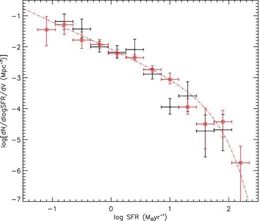
We make no attempt to fit a Schechter function to the SFR function that results from the magphys-derived SFRs, though a fit is shown to the SFR function derived by a direct scaling of the total IR luminosity (red line in Fig. 12). We notice, however, that the faint-end slope of the SFR function, α_SFR ≃ −2.3, is very steep. In fact, the integral to zero SFR of this function would diverge, so the slope has to flatten at lower SFRs. Interestingly, an analogous behaviour is not required for the total IR luminosity nor the dust mass functions. Therefore, objects with ever decreasing SFRs make a diminishing contribution to the total SFR density. This is consistent with the idea of a critical star formation density (Kennicutt 1989) below which star formation cannot take place. In this picture, the range of SFRs in the local Universe is more limited than the range of total IR luminosities as the low end of the IR luminosity function is preferentially occupied by objects whose dust is heated by the old stellar population.

GLOBAL VALUES FOR THE LOCAL UNIVERSE

Dust mass density

The best-fitting Schechter parameters for our preferred model can be used to derive the total dust mass density of the local Universe (within galaxies) using the relation:

\begin{equation} M_{\rm d,tot} = \int _{0}^{\infty }\,M\,\Phi (M)\,\mathrm{d}M = \phi _d^*\,M_{\rm d}^*\,\Gamma (2+\alpha ). \end{equation}

(10)

This gives a value of M_d,tot = (7.0 ± 1.4) × 10⁵ M_⊙ Mpc⁻³, which compares to a value of 1.4 × 10⁵ M_⊙ Mpc⁻³ determined by Dunne et al. (2011). The discrepancy is partly accounted for by the different value of κ_d used by these authors which gives dust masses lower by a factor of 2. Scaling their value results in a dust mass density of 2.8 × 10⁵. The remaining discrepancy appears to be in the larger numbers of low dust mass galaxies which we find. Driver et al. (2007) estimate a value of (5.3 ± 1.7) × 10⁵ M_⊙ Mpc⁻³ based on optical data by assuming a fixed value for the ratio of B-band luminosity to dust mass in the sample described by Popescu et al. (2002). As the dust masses of Popescu et al. (2002) are actually based on the older graphite–silicate dust model (see Section 3.1) this value should also be scaled by a factor of 2, giving (10.6 ± 3.4) × 10⁵ M_⊙ Mpc⁻³, in good agreement with our estimate.

Infrared luminosity density

Because the faint-end slope of the total IR luminosity function is quite close to −2 (α = −1.78), integrating the Schechter function, as done for the dust mass function, would result in an unreliable estimate of the total IR luminosity density of the local Universe. Instead we prefer to directly sum the measured points of the function to determine the sum for log (L_IR) ≥ 8.6. Doing this we obtain (1.74 ± 0.33) × 10⁸ L_⊙ Mpc⁻³. The same operation for the luminosity function found by Sanders et al. (2003) (also shown in Fig. 11) gives a value of (1.26 ± 0.08) × 10⁸ L_⊙ Mpc⁻³. Our determination is in good agreement with the recent value of (1.54 ± 0.26) × 10⁸ L_⊙ Mpc⁻³ estimated by Driver et al. (2012) but somewhat higher than the |$8.5^{+1.5}_{-2.3} \times 10^{7}\,{\rm L}_{{\odot }}\,\mathrm{Mpc}^{-3}$| found by Goto et al. (2011) using AKARI data, consistent with our finding that the AKARI photometry is systematically low (see Section 2.2.2).

Star formation rate density

In order to estimate the total SFR density of the local Universe, we simply sum the measured points of the SFR function in Fig. 12. We find a value of 0.0216 ± 0.0093 M_⊙ yr⁻¹ Mpc⁻³ for objects with SFR ≥ 0.1 M_⊙ yr^{− 1} (were we to have based this estimate on SFRs derived simply by scaling L_IR – red points in Fig. 12 – we would have found a value of 0.0201 ± 0.0045 M_⊙ yr⁻¹ Mpc⁻³). Our value is consistent with the range of values found in recent studies (see e.g. Bothwell et al. 2011, for a summary of recent values) as long as the SFR function flattens for SFR < 0.1 M_⊙ yr⁻¹ so that the contribution from low SFR systems is small. As discussed in Section 4.3, such a flattening of the faint-end slope is consistent with the idea of a star formation density threshold below which star formation does not occur.

SIMPLE GREY BODY FITS

To compare our results with those of previous analyses that relied on simple grey body (modified blackbody) fits of far-IR to sub-mm data we have also adopted this kind of model, adopting one- or two-temperature grey bodies. This also allows us to investigate the effect of varying the dust emissivity index, β, for which magphys uses fixed values. The uncertainty on β may contribute substantially to the error budget on parameters derived from the fits.

For these fits, we include only data at λ ≥ 60 μm (or λ ≥ 100 μm for single-temperature grey bodies). The photometric data at shorter wavelengths are left out because they are dominated by other components: stochastically heated very small grains and PAH molecules. Dealing with these components would require a much more sophisticated model. In fact a simple modified blackbody rarely fits the 25 μm IRAS point.

Single-temperature grey bodies

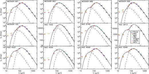
We first consider a single-temperature grey body using only data at wavelengths λ ≥ 100 μm, so as to minimize the influence of a warmer dust component. However, we do not include the Planck 217 GHz (1382 μm) point in the fits as there is a possibility that flux densities at this frequency include contributions from other components (e.g. free–free emission) or are overestimated (see below). All galaxies had at least three data points with these constraints. We fitted for the dust mass, temperature and β, except for objects which lacked data at either 100 or 160 μm (for which the temperature would be very poorly constrained). For the four objects without data at these wavelengths we fixed the temperature at the median value found for the other galaxies (21.0 K) and fitted only for the mass and β. Some illustrative examples of the fits obtained are shown in Fig. 13. The distribution of dust temperature, mass and β are shown in Fig. 14. The median value of β is 1.83, and the median dust mass is 6.0 × 10⁷ M_⊙.

Figure 13.

Open in new tab Download slide

Some example single-temperature grey body fits. Only points at λ ≥ 100 μm are taken into account in the fitting procedure (see the text).

Figure 14.

Open in new tab Download slide

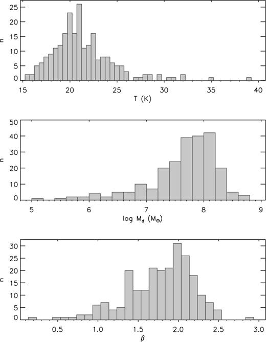
Distributions of temperature, mass and β for single-temperature grey body fits to our sample galaxies. The values are the results of fits to data at wavelengths between 100 and 850 μm (353 GHz) inclusive.

Fig. 15 shows the relation between the fitted values of the dust temperature and β when the value of β is held fixed at various values. We see an anticorrelation between the two, showing that there is clearly a degeneracy between the two parameters. This degeneracy was also noted by (Galametz et al. 2012), and Shetty et al. (2009) showed that an inverse correlation between the dust temperature T_d and β naturally arises from least-squares fits due to the uncertainties, even for sources with a single T_d and β.

Figure 15.

Open in new tab Download slide

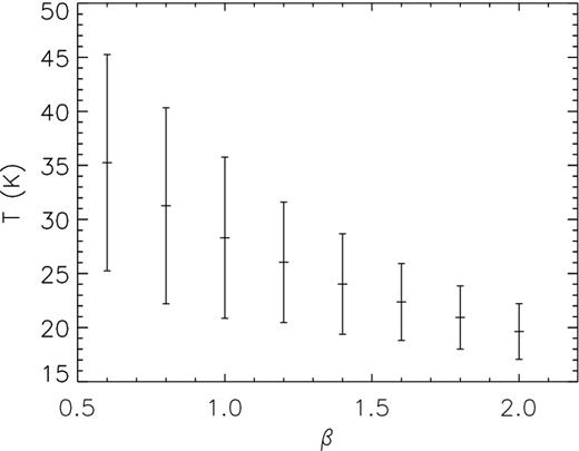
Median and standard deviation of the temperature distributions for single-component-modified blackbody fits in which β is fixed at various values.

Despite this degeneracy, previous studies have shown evidence for a real anticorrelation in Galactic H ii regions (Anderson et al. 2010; Rodón et al. 2010), cold clumps (Désert et al. 2008), Galactic cirrus (Dupac et al. 2003; Veneziani et al. 2010), the Galactic plane as a whole (Paradis et al. 2010), and galaxies observed by Planck (Planck Collaboration XVI 2011) and Herschel (Galametz et al. 2012). The effect has also been reproduced in the laboratory (Coupeaud et al. 2011).

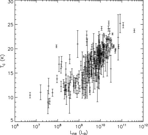
The correlation we find between L_FIR and β (lower panel of Fig. 16; correlation coefficient 0.55 with a chance probability of 4 × 10⁻⁹), and indeed the correlation we do not see between L_FIR and T_d, therefore only show that some combination of β and T_d is correlated with L_FIR.

Figure 16.

Open in new tab Download slide

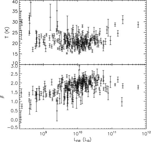
Temperature and dust emissivity index β as a function of L_FIR for single-temperature grey body fits. L_FIR is calculated by integrating the fitted curve from 40 to 500 μm.

A single-component dust temperature that does not correlate with L_IR was also found by Dunne et al. (2011), who studied galaxies in the H–ATLAS survey using Herschel data, and Planck Collaboration XVI (2011). However, for the samples of galaxies studied by Dunne et al. (2000) and Dale et al. (2001) using 850 μm SCUBA data a correlation was found. Likewise, a clear increase of the peak frequency of the dust emission (hence of the effective dust temperature) with L_IR was reported by Smith et al. (2012).

Although it may be the case that there is a real anticorrelation between T_d and β (and indeed we find the two to be anticorrelated when both are left free to vary), Fig. 15 illustrates the dangers of fitting both T_d and β. A good fit to the data can be obtained, even if the chosen (or fitted) β is too low, by assuming a higher dust temperature: χ² fits underestimating β will naturally overestimate T_d or vice versa. A similar conclusion was previously reached by Sajina et al. (2006) (see their appendix C). We will come back to this issue in Section 6.2.

Two-temperature grey bodies

Of course, any galaxy will actually have dust at several temperatures so a single component is just a simplification. In order to investigate to what extent our fitted parameters may be influenced by the addition of a warmer dust component we also fitted our sample galaxies with two grey bodies, representing the cool and warm dust components. Due to the larger number of parameters to fit, we fixed β = 2 and fitted for the two temperatures and the two masses. As we are now fitting also for warmer dust, we included data down to 60 μm in the fits, and if there were no data at either 60 or 70 μm we actually attempted no fit at all (five objects: IC 0750, NGC 3423, NGC 3646, NGC 3813, NGC 4145).

Even with the 60 μm point the warm component is often difficult to constrain, perhaps because the ‘hot’ component due to very small grains may contribute substantially to the 60 μm flux density. To mitigate this problem we have constrained warm dust temperatures to be below 60 K.

Fig. 17 shows some example fits and Fig. 18 summarizes the results of these fits. The median temperature of the cold component is 17.8 K (with 67 per cent of objects having temperatures between 13.0 and 20.6 K) and that of the warm component is 34.1 K, in excellent agreement with estimates by Planck Collaboration XVI (2011). The mass derived for the warm component is typically two orders of magnitude below that of the cool component. As illustrated by Fig. 19, the dust mass estimated from the two-temperature grey body fits is in very good agreement with that from magphys. The median dust mass in the two-component model, 8.0 × 10⁷ M_⊙, is also very close the magphys median (≃7.8 × 10⁷ M_⊙). The luminosity of the warm component is typically about 1/3 of that of the cool component, slightly less than in the magphys case (where it was about 1/2), consistent with the slightly lower derived temperatures for the warm component.⁷

Figure 17.

Open in new tab Download slide

Some example two-component grey-body fits. Only points at λ ≥ 60 μm are taken into account in the fitting procedure (see the text).

Figure 18.

Open in new tab Download slide

Distributions of temperature and mass for two-component grey body models with β fixed at 2. Values for the cold dust component are shown in blue, and those for the warm component in red. For 73 galaxies the temperature of the hot component was 60 K, the maximum allowed value. These objects are highlighted by darker red shading.

Figure 19.

Open in new tab Download slide

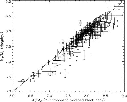
Comparison of dust masses derived from simple two-component grey body fits and those derived by magphys. The values from the latter have been multiplied by a factor of 2 to allow for the different values of the dust mass opacity coefficient, κ_d, used (see the text).

On the other hand, the median dust mass in the two-component model is slightly higher than that found in the case of single-component fits (6.0 × 10⁷ M_⊙). This difference is expected because of the dust mass/temperature degeneracy: the amount of dust mass needed to yield a given emission decreases with increasing dust temperature, and the temperature of the cold dust (that dominates the mass) decreases in the two-component case. The difference among the median dust masses, however, is only a factor of 1.33.

Although the addition of a second component is necessary to fit flux densities at λ ≲ 80 μm the quality of the fit to the data for λ ≥ 80 μm is actually slightly worse in the case of the two-component model where β is fixed at a value of 2.0 compared to the single-component fit where β is free to vary (χ² increases from 16 to 22 for the λ ≥ 80 μm data points). Therefore, a single component is perfectly adequate to describe the long wavelength data. Interestingly, the median value of β found for the sub-set of objects with at least five measured points at λ ≥ 80 μm is 1.95, very close to the often used value of 2.0.

The introduction of a second dust component causes the appearance of a strong correlation between the temperature of the cold component and L_IR (Fig. 20), in contrast to what was seen in the single-component case. Although this correlation may be real we cannot be sure that it is not caused by a trend in β (held fixed here) with L_IR, as the two parameters are clearly degenerate (Fig. 15). No correlation is found with the temperature of the warm component.

Figure 20.

Open in new tab Download slide

Temperature of the cold dust component versus the IR luminosity (40-1000 μm) in the two-component grey body fits.

Excess emission at 217 GHz

A distinctive property of the present sample is the availability of 850 μm (353 GHz) flux densities for 181 (77 per cent) sources, and of 1.38 mm (217 GHz) flux densities for 47 (20 per cent). These long-wavelength data may provide tight constraints on the dust emissivity index β. On the other hand, although bright radio galaxies were excluded from the sample there is the possibility of a significant contribution at 217 GHz from either a weak nuclear radio source or from free–free emission. A detection of free–free emission, that has turned out to be elusive so far, would be of interest per se since it is a direct tracer of star formation, not affected by dust extinction. We caution however, that although the sample is 80 per cent complete at 545 GHz, there is no flux limit applied to the 217 GHz measurements.

Of the 47 objects with 217 GHz data we find that the flux density is in excess of the expectation from the dust emission SED by more than the nominal error on the datum in 38 cases for the two-component fits with β = 2 (and also if β = 1.5 for the warm component). Even in the case of one-component models where β is allowed to vary, a similar number of excess flux densities result. Flux densities at 217 GHz are therefore not well fitted by modified blackbody fits, and in fact were excluded from the fits described in Section 6.1. We remind the reader that the Planck flux densities have been corrected statistically for CO emission as described in Negrello et al. (2013), and note that a clear excess is present independent of whether or not the correction is applied.

However, only 12 of the objects with measured 217 GHz flux densities are above the 80 per cent completeness limits at this frequency (S_{lim, 217} = 497 mJy); all show the excess. Two of them, NGC 253 and M82, have been studied in detail by Peel et al. (2011), who found evidence for free–free contributions at 217 GHz of ∼13 per cent and ∼25 per cent, respectively. A third one is M77, which is known to host a nuclear radio source; it has the highest excess (≃30 per cent). The significance of the excess for the other nine sources is low, especially if we take into account that the source extraction is made on filtered maps (see, e.g. Herranz & Vielva 2010). This procedure greatly improves the source detection efficiency but leads to an underestimate of the measurement errors. Indeed Negrello et al. (2013) compared large numbers of Planck flux densities at 857 and 545 GHz with Herschel 350 and 500 μm data and showed that the rms deviation from the Herschel flux densities (which have far higher S/N ratios) was ∼30 per cent, substantially larger than expected from the nominal errors. Although we do not have a sample with which to compare the Planck 217 GHz flux densities, it is unlikely that the situation at this frequency is any different. None of the nine sources show an excess ≥30 per cent; typical values are ≃20 per cent. On the other hand, the fact that all sources above S_{lim, 217} = 497 mJy do show hints of an excess may constitute statistical evidence of an additional minor contribution, possibly due to free–free emission as clearly seen for NGC 253 and M 82.

Synchrotron emission could also contribute significantly to the 217 GHz flux densities. We estimate the synchrotron contribution at 217 GHz by extrapolating the measured radio flux densities and assuming that the spectral index measured in the 1–20 GHz range remains the same at higher frequencies. This is most likely a generous upper limit since synchrotron spectra generally steepen at higher frequencies due to electron ageing effects. We find a median contribution of 1.9 per cent (mean 3.3 per cent). A significant excess of 29 per cent is found only for M77. For M82, NGC 253 and another galaxy not in our sample (NGC 4945) Peel et al. (2011) indeed find that the synchrotron contribution is negligible at 217 GHz, compared to free–free.

As a blackbody with a peak at 217 GHz has a temperature of 2.1 K, it will clearly be difficult to have a substantial contribution at this frequency from an additional cold dust component with a physically realistic dust temperature without producing an (unobserved) excess also at the higher frequencies. It is, in principle, possible to fit the 217 GHz flux densities by adding a dust component with a very low β ∼ 1, that dominates increasingly at longer wavelengths, but such a model would be rather contrived.

The analysis by Negrello et al. (2013) also showed that flux densities below the 80 per cent completeness limit are substantially overestimated, as a result of ‘flux boosting’ due to source confusion. The ‘excess’ found for sources below the 217 GHz 80 per cent completeness limits, whose median value is 28 per cent, is fully compatible with the same effect.

The value of β and very cold dust

As we saw in Section 6.2, if we limit our sample to those objects with most data (for example the 84 objects with five or more flux densities at ≥ 80 μm), we find that the median fitted value of β for the one-component fits is 1.95. Therefore, our fits for the one- and two-component models in the long-wavelength part of the SEDs are almost identical when the latter have β fixed at 2. Although the 217 GHz point is often poorly fitted (see Section 6.3), there is little to choose between the one- and two-component models in the Rayleigh–Jeans part of the spectrum and a value of β = 2 seems to describe very well the emission from the cool dust component. Although strong evidence for a secondary dust component with a lower value of β has been found using Planck data of the Small Magellanic Cloud (Planck Collaboration XVII 2011), we find no evidence that this is a general property of dust in nearby galaxies.

Although we do find sources with dust temperatures as low as ∼10 K in our simple two-component fits⁸ (consistent with Planck Collaboration XVI 2011) we find no evidence of an additional very cold dust component (6–10 K) similar to that reported in some dwarf galaxies (Galliano et al. 2005; Grossi et al. 2010; O'Halloran et al. 2010; Planck Collaboration XVII 2011). Specifically, the addition of a very cold dust component with β = 2 with a temperature constrained to lie in the range 6–15 K does not lower the χ² value with respect to the single-component fit.

We might ask the question, ‘How much very cold dust could potentially exist in star-forming galaxies and remain undetected with the existing data?’. For example, if we fix the temperature of the very cold dust at 6 K for the 84 objects with five or more flux densities at ≥ 80 μm, we obtain acceptable fits where the mass of the very cold dust is of the order of that in the ∼20 K component. However, this is simply because the long-wavelength fluxes are anyway dominated by the ∼20 K component. As mentioned above, the single-component fits, in which β is free to vary are always better fits to the data.

Therefore, although the presence of a very cold dust component cannot be ruled out, and there is a significant degeneracy between β and the very cold dust mass, we find no evidence for very cold dust in the data. In no object is there a ‘bump’ in the Rayleigh–Jeans part of the spectrum that could not be explained by variations in β. Such very cold dust may be a phenomenon found only in dwarf galaxies, and perhaps connected to their low metallicity. Alternatively, the excess emission that has been interpreted as cold dust in studies such as those cited above, may reflect a dust component with a low value of β.

CONCLUSIONS

We have used multifrequency data to construct the SED for a flux-limited sample of 234 local galaxies selected from the Planck ERCSC at 545 GHz. This sample is biased towards dusty objects with respect to analogous samples selected in the optical, but is ideally suited to investigating the SFR and dust mass distribution of the z = 0 Universe. We have fitted various models to the SEDs to derive global parameters for the dust and related parameters in each object. We reach the following conclusions.

We find a median dust mass of 7.80 × 10⁷ M_⊙ for our sample that has a median stellar mass of 1.80 × 10¹⁰ M_⊙. The median dust mass fraction is 0.0046.
Within our sample the dust mass is well correlated with the H i mass. The median ratio |$M_{\rm d}/M_{\rm H\,{\small {I}}}$| is 0.022. The ratios of M_d and |$M_{\rm H\,{\small {I}}}$| to the stellar mass are anticorrelated with the stellar mass. Therefore, more massive galaxies tend to have proportionately less ISM in general. The SFR is correlated with dust mass but not with the stellar mass.
The median cold and warm dust temperatures yielded by magphys (da Cunha et al. 2008) are 17.7 K and 43 K, respectively but the magphys requirement that the warm dust temperature is ≥30 K may bias high the estimates. When two simple grey body dust components are considered a median cold dust temperature of 17.8 K, very close to the magphys estimate is recovered, but the median warm dust temperature decreases to 34.1 K. Although the warm component typically contributes between approximately one quarter to one-third of the total IR luminosity, it accounts for only ∼1 per cent of the dust mass.
We find a correlation between the SFR per unit dust mass and the cold dust temperature (but not with the warm dust temperature), suggesting that a significant fraction of even the cold dust emission is powered by ongoing star formation. This dust is probably physically associated with both star-forming regions and cirrus. The quiescent disc population appears to play a secondary role as a dust heating source, especially for sources with warmer dust temperatures.
The far-IR emission of local star-forming galaxies at wavelengths λ ≳ 100 μm is very well characterized by a single modified blackbody with β in the range 1–2.5. However, fits in which β is fixed at a value of 2 fit the data almost as well. This reflects a degeneracy between T_d and β inherent to the single-temperature model. Dust masses for a single-temperature model in which both T_d and β are free parameters are about 30 per cent lower than in a two-component model in which β = 2 and is fixed.
We have used the bivariate technique to compute the dust mass function, the total IR luminosity function and the SFR function of local galaxies. The differences that we find in the dust mass function from previous works are mainly due to the different value used for the dust mass absorption coefficient, κ_d, which results in higher masses. Below 10⁷ M_⊙ the function is similar to that found by Vlahakis et al. (2005), whereas above 10⁷ M_⊙ it is very similar to that found by Dunne et al. (2011) for z < 0.1. We find that the mean dust mass density of the local Universe, for dust within galaxies, is 7.0 ± 1.4 × 10⁵ M_⊙ Mpc⁻³, 2.5 times the estimate by Dunne et al. (2011) based on Herschel data. The difference is mostly due to the contribution of low-M_d galaxies, for which we find a number density significantly higher than found by Dunne et al. (2011).
Our estimate of the local infrared luminosity function is in very good agreement with previous estimates based on IRAS data alone and with that obtained when we limit the data of our present sample to include only IRAS data. The total IR luminosity density of the local Universe is found to be (1.74 ± 0.33) × 10⁸ L_⊙ Mpc⁻³.
We find a total SFR for the local Universe of (0.0216 ± 0.0093) M_⊙ yr⁻¹ Mpc⁻³ for objects with SFR ≥ 0.1 M_⊙ yr⁻¹.
Flux densities measured in the Planck 217 GHz band typically show an excess above model fits that we interpret as statistical evidence for a contribution from free–free emission at a level of ≲20 per cent. Synchrotron emission from our sources in this band is negligible, except for M77, which has a weak central radio jet.
Though we find galaxies with cold dust temperatures as low as 10 K, we find no evidence for an additional very cold component (6–10 K) analogous to that identified in dwarf galaxies.

We gratefully acknowledge many constructive comments by the anonymous referee that helped to substantially improve this paper. This work was supported in part by ASI/INAF agreement I/072/09/0. JGN acknowledges financial support from Spanish CSIC for a JAE-DOC fellowship. JGN, LB and LT acknowledge partial financial support from the Spanish Ministerio de Ciencia e Innovacion under the projects AYA2010-21766-C03-01 and by the Consolider Ingenio-2010 Programme, project CSD2010-00064. This research has made use of the NASA/IPAC Extragalactic Database (NED) which is operated by the Jet Propulsion Laboratory, California Institute of Technology, under contract with the National Aeronautics and Space Administration. This publication makes use of data products from the Wide-field Infrared Survey Explorer, which is a joint project of the University of California, Los Angeles, and the Jet Propulsion Laboratory/California Institute of Technology, funded by the National Aeronautics and Space Administration. We acknowledge the usage of the HyperLeda data base (http://leda.univ-lyon1.fr).

1

This is the notation used in the Wise All Sky Data Release where the ‘?’ is to be replaced by either 1, 2, 3 or 4 depending on the observing band.

2

In cases where more than one flux density measurement was available at a given wavelength, the values were averaged with a weight inversely proportional to the error on the datum.

3

http://leda.univ-lyon1.fr/

4

Nonetheless, the fact that our sample is selected in the sub-mm does mean that we are more likely to include objects at the high end of the |$M_{\rm d}/M_{\rm H\,{\small {I}}}$| distribution.

5

We also note that there is only a very weak correlation between T_c and log (SFR), and T_c and log (SFR/M_*).

6

Whether or not this is the case, we do not wish to implicitly assume that there is a one-to-one relation between IR luminosity and SFR.

7

Only objects where the temperature of the warm component was less than the 60 K model upper limit were considered in this calculation.

8

Not below 12 K for the sub-set of objects with five or more data points at λ ≥ 80 μm.

REFERENCES

Anderson

L. D.

, et al. ,

A&A

,

2010

, vol.

518

pg.

L99

Crossref

Search ADS

Auld

R.

, et al. ,

MNRAS

,

2013

, vol.

428

pg.

1880

Crossref

Search ADS

Bell

E. F.

,

de Jong

R. S.

. ,

MNRAS

,

2000

, vol.

312

pg.

497

Crossref

Search ADS

Bendo

G. J.

,

Galliano

F.

,

Madden

S. C.

. ,

MNRAS

,

2012

, vol.

423

pg.

197

Crossref

Search ADS

Boselli

A.

, et al. ,

PASP

,

2010

, vol.

122

pg.

261

Crossref

Search ADS

Bothwell

M. S.

, et al. ,

MNRAS

,

2011

, vol.

415

pg.

1815

Crossref

Search ADS

Brinchmann

J.

,

Charlot

S.

,

White

S. D. M.

,

Tremonti

C.

,

Kauffmann

G.

,

Heckman

T.

,

Brinkmann

J.

. ,

MNRAS

,

2004

, vol.

351

pg.

1151

Crossref

Search ADS

Bruzual

G.

,

Charlot

S.

. ,

MNRAS

,

2003

, vol.

344

pg.

1000

Crossref

Search ADS

Chabrier

G.

. ,

PASP

,

2003

, vol.

115

pg.

763

Crossref

Search ADS

Charlot

S.

,

Fall

S. M.

. ,

ApJ

,

2000

, vol.

539

pg.

718

Crossref

Search ADS

Ciesla

L.

, et al. ,

A&A

,

2012

, vol.

543

pg.

A161

Crossref

Search ADS

Cortese

L.

, et al. ,

A&A

,

2012

, vol.

540

pg.

A52

Crossref

Search ADS

Coupeaud

A.

, et al. ,

A&A

,

2011

, vol.

535

pg.

A124

Crossref

Search ADS

da Cunha

E.

,

Charlot

S.

,

Elbaz

D.

. ,

MNRAS

,

2008

, vol.

388

pg.

1595

Crossref

Search ADS

da Cunha

E.

,

Eminian

C.

,

Charlot

S.

,

Blaizot

J.

. ,

MNRAS

,

2010

, vol.

403

pg.

1894

Crossref

Search ADS

Dale

D. A.

,

Helou

G.

,

Contursi

A.

,

Silbermann

N. A.

,

Kolhatkar

S.

. ,

ApJ

,

2001

, vol.

549

pg.

215

Crossref

Search ADS

Dale

D. A.

, et al. ,

ApJ

,

2005

, vol.

633

pg.

857

Crossref

Search ADS

Davies

J. I.

, et al. ,

A&A

,

2010

, vol.

518

pg.

L48

Crossref

Search ADS

Davies

J. I.

, et al. ,

MNRAS

,

2012

, vol.

419

pg.

3505

Crossref

Search ADS

de Jong

T.

,

Clegg

P. E.

,

Rowan-Robinson

M.

,

Soifer

B. T.

,

Habing

H. J.

,

Houck

J. R.

,

Aumann

H. H.

,

Raimond

E.

. ,

ApJ

,

1984

, vol.

278

pg.

L67

Crossref

Search ADS

de Vaucouleurs

G.

,

de Vaucouleurs

A.

,

Corwin

H. G.

,

Buta

R. J.

,

Paturel

G.

,

Fouque

P.

. ,

The Third Reference Catalog of Bright Galaxies

,

1991

New York

Springer-Verlag

Google Scholar

Google Preview

OpenURL Placeholder Text

WorldCat

Désert

F.-X.

, et al. ,

A&A

,

2008

, vol.

481

pg.

411

Crossref

Search ADS

Draine

B. T.

. ,

ARA&A

,

2003

, vol.

41

pg.

241

Crossref

Search ADS

Draine

B. T.

,

Lee

H. M.

. ,

ApJ

,

1984

, vol.

285

pg.

89

Crossref

Search ADS

Draine

B. T.

, et al. ,

ApJ

,

2007

, vol.

663

pg.

866

Crossref

Search ADS

Driver

S. P.

,

Allen

P. D.

,

Liske

J.

,

Graham

A. W.

. ,

ApJ

,

2007

, vol.

657

pg.

L85

Crossref

Search ADS

Driver

S. P.

, et al. ,

MNRAS

,

2012

, vol.

427

pg.

3244

Crossref

Search ADS

Dunne

L.

,

Eales

S.

,

Edmunds

M.

,

Ivison

R.

,

Alexander

P.

,

Clements

D. L.

. ,

MNRAS

,

2000

, vol.

315

pg.

115

Crossref

Search ADS

Dunne

L.

, et al. ,

MNRAS

,

2011

, vol.

417

pg.

1510

Crossref

Search ADS

Dupac

X.

, et al. ,

A&A

,

2003

, vol.

404

pg.

L11

Crossref

Search ADS

Galametz

M.

, et al. ,

MNRAS

,

2012

, vol.

425

pg.

763

Crossref

Search ADS

Galliano

F.

,

Madden

S. C.

,

Jones

A. P.

,

Wilson

C. D.

,

Bernard

J.-P.

. ,

A&A

,

2005

, vol.

434

pg.

867

Crossref

Search ADS

González

V.

,

Labbé

I.

,

Bouwens

R. J.

,

Illingworth

G.

,

Franx

M.

,

Kriek

M.

,

Brammer

G. B.

. ,

ApJ

,

2010

, vol.

713

pg.

115

Crossref

Search ADS

Goto

T.

, et al. ,

MNRAS

,

2011

, vol.

410

pg.

573

Crossref

Search ADS

Graciá-Carpio

J.

,

García-Burillo

S.

,

Planesas

P.

,

Fuente

A.

,

Usero

A.

. ,

A&A

,

2008

, vol.

479

pg.

703

Crossref

Search ADS

Grossi

M.

, et al. ,

A&A

,

2010

, vol.

518

pg.

L52

Crossref

Search ADS

Heidmann

J.

,

Heidmann

N.

,

de Vaucouleurs

G.

. ,

MNRAS

,

1972

, vol.

75

pg.

85

Helou

G.

. ,

ApJ

,

1986

, vol.

311

pg.

L33

Crossref

Search ADS

Herranz

D.

,

Vielva

P.

. ,

IEEE Signal Process. Mag.

,

2010

, vol.

27

pg.

67

Crossref

Search ADS

Herranz

D.

, et al. ,

A&A

,

2013

, vol.

549

pg.

A31

Crossref

Search ADS

Hildebrand

R. H.

. ,

Q. J. R. Astron. Soc.

,

1983

, vol.

24

pg.

267

Huchtmeier

W. K.

,

Wendker

H. J.

,

Tammann

G. A.

. ,

A&A

,

1976

, vol.

46

pg.

381

Jarrett

T. H.

,

Chester

T.

,

Cutri

R.

,

Schneider

S. E.

,

Huchra

J. P.

. ,

AJ

,

2003

, vol.

125

pg.

525

Crossref

Search ADS

Kennicutt

R. C.

,

Evans

N. J.

. ,

ARA&A

,

2012

, vol.

50

pg.

531

Crossref

Search ADS

Kennicutt

R. C.

Jr

. ,

ApJ

,

1989

, vol.

344

pg.

685

Crossref

Search ADS

Kennicutt

R. C.

Jr

. ,

ARA&A

,

1998

, vol.

36

pg.

189

Crossref

Search ADS

Kennicutt

R. C.

, et al. ,

PASP

,

2011

, vol.

123

pg.

1347

Crossref

Search ADS

Lagache

G.

,

Abergel

A.

,

Boulanger

F.

,

Puget

J.-L.

. ,

A&A

,

1998

, vol.

333

pg.

709

Lapi

A.

, et al. ,

ApJ

,

2011

, vol.

742

pg.

24

Crossref

Search ADS

Lisenfeld

U.

, et al. ,

A&A

,

2007

, vol.

462

pg.

507

Crossref

Search ADS

Negrello

M.

, et al. ,

MNRAS

,

2013

, vol.

429

pg.

1309

Crossref

Search ADS

O'Halloran

B.

, et al. ,

A&A

,

2010

, vol.

518

pg.

L58

Crossref

Search ADS

Paradis

D.

, et al. ,

A&A

,

2010

, vol.

520

pg.

L8

Crossref

Search ADS

Paturel

G.

,

Petit

C.

,

Prugniel

P.

,

Theureau

G.

,

Rousseau

J.

,

Brouty

M.

,

Dubois

P.

,

Cambrésy

L.

. ,

A&A

,

2003

, vol.

412

pg.

45

Crossref

Search ADS

Peel

M. W.

,

Dickinson

C.

,

Davies

R. D.

,

Clements

D. L.

,

Beswick

R. J.

. ,

MNRAS

,

2011

, vol.

416

pg.

L99

Crossref

Search ADS

Planck

Collaboration VII

. ,

A&A

,

2011

, vol.

536

pg.

A7

Crossref

Search ADS

Planck

Collaboration XVI

. ,

A&A

,

2011

, vol.

536

pg.

A16

Crossref

Search ADS

Planck

Collaboration XVII

. ,

A&A

,

2011

, vol.

536

pg.

A17

Crossref

Search ADS

Planck Collaboration

,

The Explanatory Supplement to the Planck Early Release Compact Source Catalogue (ESA)

,

2011

available at: http://www.sciops.esa.int/SA/PLANCK/docs/ERCSC_explanatory_supplement.pdf

Popescu

C. C.

,

Tuffs

R. J.

,

Völk

H. J.

,

Pierini

D.

,

Madore

B. F.

. ,

ApJ

,

2002

, vol.

567

pg.

221

Crossref

Search ADS

Rice

W.

,

Lonsdale

C. J.

,

Soifer

B. T.

,

Neugebauer

G.

,

Kopan

E. L.

,

Lloyd

L. A.

,

de Jong

T.

,

Habing

H. J.

. ,

ApJS

,

1988

, vol.

68

pg.

91

Crossref

Search ADS

Rodón

J. A.

, et al. ,

A&A

,

2010

, vol.

518

pg.

L80

Crossref

Search ADS

Sajina

A.

,

Scott

D.

,

Dennefeld

M.

,

Dole

H.

,

Lacy

M.

,

Lagache

G.

. ,

MNRAS

,

2006

, vol.

369

pg.

939

Crossref

Search ADS

Sanders

D. B.

,

Mirabel

I. F.

. ,

ARA&A

,

1996

, vol.

34

pg.

749

Crossref

Search ADS

Sanders

D. B.

,

Mazzarella

J. M.

,

Kim

D.-C.

,

Surace

J. A.

,

Soifer

B. T.

. ,

AJ

,

2003

, vol.

126

pg.

1607

Crossref

Search ADS

Serjeant

S.

,

Pearson

C.

,

White

G. J.

,

Smith

M. W. L.

,

Doi

Y.

. ,

2012

preprint (arXiv:1208.3631)

Shetty

R.

,

Kauffmann

J.

,

Schnee

S.

,

Goodman

A. A.

. ,

ApJ

,

2009

, vol.

696

pg.

676

Crossref

Search ADS

Skibba

R. A.

, et al. ,

ApJ

,

2011

, vol.

738

pg.

89

Crossref

Search ADS

Smith

D. J. B.

, et al. ,

MNRAS

,

2012

, vol.

427

pg.

703

Crossref

Search ADS

Soifer

B. T.

,

Boehmer

L.

,

Neugebauer

G.

,

Sanders

D. B.

. ,

AJ

,

1989

, vol.

98

pg.

766

Crossref

Search ADS

Surace

J. A.

,

Sanders

D. B.

,

Mazzarella

J. M.

. ,

AJ

,

2004

, vol.

127

pg.

3235

Crossref

Search ADS

Tremonti

C. A.

, et al. ,

ApJ

,

2004

, vol.

613

pg.

898

Crossref

Search ADS

Veneziani

M.

, et al. ,

ApJ

,

2010

, vol.

713

pg.

959

Crossref

Search ADS

Vlahakis

C.

,

Dunne

L.

,

Eales

S.

. ,

MNRAS

,

2005

, vol.

364

pg.

1253

Crossref

Search ADS

Whittet

D. C. B.

.

Tayler

R. J.

,

White

R. E.

. ,

Dust in the Galactic Environment

,

1992

Bristol

IoP Publishing

pg.

306

Wright

E. L.

, et al. ,

AJ

,

2010

, vol.

140

pg.

1868

Crossref

Search ADS

Yamamura

I.

,

Makiuti

S.

,

Ikeda

N.

,

Fukuda

Y.

,

Oyabu

S.

,

Koga

T.

,

White

G. J.

. ,

yCat

,

2010

, vol.

2298

pg.

0

Download all slides

Month:	Total Views:
January 2017	1
February 2017	5
March 2017	5
April 2017	1
May 2017	7
June 2017	8
July 2017	6
August 2017	3
September 2017	15
October 2017	16
November 2017	9
December 2017	7
January 2018	9
February 2018	8
March 2018	35
April 2018	32
May 2018	22
June 2018	27
July 2018	17
August 2018	12
September 2018	3
October 2018	21
November 2018	23
December 2018	8
January 2019	12
February 2019	13
March 2019	24
April 2019	27
May 2019	16
June 2019	11
July 2019	16
August 2019	14
September 2019	8
October 2019	20
November 2019	16
December 2019	10
January 2020	13
February 2020	14
March 2020	23
April 2020	13
May 2020	11
June 2020	9
July 2020	11
August 2020	7
September 2020	11
October 2020	6
November 2020	10
December 2020	8
January 2021	5
February 2021	18
March 2021	16
April 2021	10
May 2021	8
June 2021	11
July 2021	9
August 2021	4
September 2021	7
October 2021	8
November 2021	5
December 2021	5
January 2022	5
February 2022	4
March 2022	10
April 2022	11
May 2022	7
June 2022	7
July 2022	10
August 2022	14
September 2022	7
October 2022	13
November 2022	5
December 2022	10
January 2023	10
February 2023	5
March 2023	5
April 2023	8
May 2023	14
June 2023	10
July 2023	5
August 2023	15
September 2023	14
October 2023	8
November 2023	4
December 2023	23
January 2024	16
February 2024	11
March 2024	4
April 2024	12

Article Contents

Dust and star formation properties of a complete sample of local galaxies drawn from the Planck Early Release Compact Source Catalogue

Abstract

INTRODUCTION

SAMPLE SELECTION AND AUXILIARY DATA

Planck flux densities

Data at other wavelengths

IRAS

AKARI

WISE

Spitzer

Herschel

FITS TO THE DATA

Dust temperatures and masses

Dust, atomic gas and stellar mass

Dust mass versus SFR

SFR versus dust temperature

SFR versus LIR

DISTRIBUTION FUNCTIONS

Dust mass function

Total infrared luminosity function

Star formation rate function

GLOBAL VALUES FOR THE LOCAL UNIVERSE

Dust mass density

Infrared luminosity density

Star formation rate density

SIMPLE GREY BODY FITS

Single-temperature grey bodies

Two-temperature grey bodies

Excess emission at 217 GHz

The value of β and very cold dust

CONCLUSIONS

REFERENCES

Citations

Views

Altmetric

Email alerts

Astrophysics Data System

Citing articles via

Latest

Most Read

Most Cited

This Feature Is Available To Subscribers Only

SFR versus L_IR