


Abstract
We present results from four years of twice-weekly 15 GHz radio monitoring of about 1500 blazars with the Owens Valley Radio Observatory 40 m telescope. Using the intrinsic modulation index to measure variability amplitude, we find that, with >6σ significance, the radio variability of radio-selected gamma-ray-loud blazars is stronger than that of gamma-ray-quiet blazars. Our extended data set also includes at least 21 months of data for all AGN with ‘clean’ associations in the Fermi Large Area Telescope First AGN Catalog, 1LAC. With these additional data, we examine the radio variability properties of a gamma-ray-selected blazar sample. Within this sample, we find no evidence for a connection between radio variability amplitude and optical classification. In contrast, for our radio-selected sample we find that the BL Lac object subpopulation is more variable than the flat-spectrum radio quasar (FSRQ) subpopulation. Radio variability is found to correlate with the synchrotron peak frequency, with low- and intermediate-synchrotron-peaked blazars varying more than high-synchrotron-peaked ones. We find evidence for a significant negative correlation between redshift and radio variability among bright FSRQs.
1 INTRODUCTION
Active galactic nuclei (AGN) are among the most energetic objects in the Universe. In an AGN, a variety of energetic phenomena are driven by a supermassive black hole, fuelled by accretion from its host galaxy. Many AGN produce relativistic jets: collimated structures visible at parsec through kiloparsec scales. Relativistic beaming effects in the jets enhance the intrinsically anisotropic appearance of the AGN, adding considerable complication to their identification and to the interpretation of observations. Statistical studies involving large samples are thus essential to the study of AGN, and careful attention must be paid to selection effects (e.g. Lister & Marscher 1997).
When the jet axis of an AGN is aligned very closely to our line of sight, Doppler-enhanced jet emission dominates other emission processes and the source is classified as a blazar. Blazars emit brightly across the entire electromagnetic spectrum, with a spectral energy distribution (SED) characterized by two broad peaks. The lower peak, spanning the radio through the optical, ultraviolet or soft X-ray bands, is widely believed to be due to synchrotron emission from relativistic electrons. The upper peak, which often extends to GeV and sometimes TeV gamma-ray energies, is of less certain origin. It is most commonly ascribed to inverse Compton scattering of low-energy seed photons by the synchrotron-emitting electrons in the jet, but other models remain viable (e.g. Böttcher 2007; Boettcher 2012; Dimitrakoudis et al. 2012). The source of the low-energy seed photons is uncertain. Certainly, some of the synchrotron radiation from within the jet is reprocessed and emitted at higher energies, and models in which this process is predominant are known as synchrotron self-Compton (SSC) models. The alternative is a source of seed photons external to the jet, such as from the broad-line region, and models in which this is important are known as external Compton (EC) models.
Blazars are customarily divided into two optical subclasses, the flat-spectrum radio quasars (FSRQs) and the BL Lac objects (BL Lacs). Blazars with strong optical broad lines are classified as FSRQs, while those with no lines or weak lines are classified as BL Lacs. Although the BL Lac and FSRQ classes do seem to represent at least two distinct populations, there is evidence that this classification scheme does not accurately reflect intrinsic physical differences between sources. For example, the homogeneity of the BL Lac class has been questioned (e.g. Marchã et al. 1996; Antón & Browne 2005) and several nominal BL Lacs have been observed to meet the FSRQ definition in some epochs (Shaw et al. 2012). It remains unclear how best to define physically meaningful classes. Several alternative classifications have been proposed in recent years (e.g. Landt et al. 2004; Abdo et al. 2010c; Ghisellini et al. 2011; Meyer et al. 2011; Giommi et al. 2012).
A promising and currently popular method is to classify blazars based on the frequency of the synchrotron peak in the SED (Padovani & Giommi 1995; Abdo et al. 2010c). Blazars are divided into low-, intermediate- and high-synchrotron-peaked (LSP, ISP and HSP) sources, defined by synchrotron peaks νpk below 1014 Hz, between 1014 and 1015 Hz and above 1015 Hz, respectively. FSRQs are almost exclusively found to be LSP objects, while BL Lacs are found in all three spectral classes. HSP BL Lacs show clearly distinct gamma-ray and radio properties from FSRQs (e.g. Abdo et al. 2010b,c; Ackermann et al. 2011b; Lister et al. 2011; Linford, Taylor & Schinzel 2012b). HSP BL Lacs display higher ratios of gamma-ray to radio luminosity, lower radio core brightness temperatures, and appear to have lower jet Doppler factors (Lister et al. 2011). There is also evidence that LSP BL Lacs remain a distinct class from FSRQs, though they appear to be sometimes misidentified (Lister et al. 2011; Linford et al. 2012b).
A connection between the radio and gamma-ray emission in blazars has long been suspected, and has received renewed attention during the era of the Fermi Large Area Telescope (LAT) (e.g. Jorstad et al. 2001b; Kovalev et al. 2009; Ghirlanda et al. 2010; Mahony et al. 2010; Ackermann et al. 2011a). It is straightforward to demonstrate a statistically significant correlation between observed gamma-ray and radio luminosities or flux densities, as was done during the era of the EGRET instrument (e.g. Padovani et al. 1993; Stecker, Salamon & Malkan 1993). However, because of distance effects, the Malmquist bias, and the strong variability exhibited in blazars, such an apparent correlation may or may not correspond to an interesting intrinsic correlation (e.g. Mücke et al. 1997). Recent studies using LAT data and concurrent or nearly concurrent radio data provide strong evidence for an intrinsic correlation (Kovalev et al. 2009; Ackermann et al. 2011a). The data concurrency reduces or eliminates spurious effects from variability, and Monte Carlo statistical methods demonstrate that the correlation is not due to other biases (Ackermann et al. 2011a; Pavlidou et al. 2012). If the connection between radio and gamma-ray emission is tight enough to produce correlated variability, cross-correlations between light curves in the two bands could constrain the relative locations of the emission. A search for statistically and physically significant time-domain correlations using our data set finds a few examples, but longer time series are needed to rule out chance correlations in most cases (Max-Moerbeck et al., in preparation).
In this paper, we present results from our continuing investigation of the connection between the gamma-ray loudness of a blazar and its radio variability. In Richards et al. (2011), we used two years of data from our 15 GHz monitoring programme to find strong evidence that gamma-ray-loud blazars in our radio-selected sample were more radio variable than their gamma-ray-quiet counterparts. We also found significant differences in variability amplitudes between the radio-selected FSRQ and BL Lac populations, with the latter more radio variable. This paper re-examines these findings using an additional two years of radio data, for a total of four years. Our monitoring sample during this extended period now also contains a complete gamma-ray-selected sample, the First LAT AGN Catalog (1LAC; Abdo et al. 2010b), which allows us to compare the gamma-ray-selected FSRQ and BL Lac populations.
2 THE MONITORING PROGRAMME
Since late 2007, we have operated a fast-cadence 15 GHz radio blazar monitoring programme using the 40 m telescope at the Owens Valley Radio Observatory (OVRO). Full details of the observing programme are given in Richards et al. (2011) and Richards (2012). Total intensity flux density measurements are performed using a combined Dicke-switching and beam-switching ‘double switching’ procedure to remove receiver gain fluctuation, atmospheric and ground pick-up effects. Each flux density is measured in about 70 s, including 32 s of on-source integration time. With a total system temperature of about 55 K at zenith, including receiver, atmosphere and cosmic microwave background noise temperature contributions, this yields a typical measurement uncertainty of about 3 mJy, which is measured from the scatter of the samples in each observation. Accurate pointing is achieved by regularly peaking up on a relatively bright programme source. Residual pointing errors and other sources contribute an additional 2 per cent uncertainty, added in quadrature with the measured error for each measurement. The flux density scale is determined from regular observations of 3C 286 assuming the Baars et al. (1977) value of 3.44 Jy at 15.0 GHz, giving a 5 per cent overall scale accuracy.
The monitoring sample began with the 1158 sources north of −20° declination from the Candidate Gamma-Ray Blazar Survey (CGRaBS; Healey et al. 2008). The CGRaBS sources were systematically selected to resemble AGN (mostly blazars) associated with EGRET gamma-ray detections based on their radio spectral index, radio flux density and X-ray flux. In addition to the CGRaBS sample, we have added the radio sources associated with Fermi-LAT gamma-ray detections to our programme. The sources included in the 1LAC catalogue compose a gamma-ray-selected sample. About 44 per cent of the sources in the 1LAC sample are in the CGRaBS sample (263 of 599 at all declinations, 199 of 454 above −20°). These have been monitored since the inception of the programme. Some non-CGRaBS sources were added after appearing in the LAT Bright AGN Sample based on the 3-month Fermi-LAT results (Abdo et al. 2009). Any remaining 1LAC sources in our declination range not already being monitored were added to the programme in 2010 March.
In late 2011, we added sources in the Second LAT AGN Catalog (2LAC; Ackermann et al. 2011b) to our observing programme. Although many were already in our programme, the observation period described here does not include sufficient data to obtain robust results for some sources in the complete 2LAC sample. We therefore use 1LAC as our gamma-ray-selected sample in the studies that follow. We do, however, use the 2LAC sample to identify the subset of CGRaBS sources that are gamma-ray loud.
The CGRaBS and Fermi samples differ substantially in the ratio of the FSRQs to BL Lacs. The CGRaBS sample is dominated by FSRQs (70 per cent FSRQs versus 11 per cent BL Lacs), similar to the ratio found by EGRET (Hartman et al. 1999; Dermer 2007). Fermi-selected blazar samples are more evenly split, both for 1LAC (40 per cent FSRQs versus 49 per cent BL Lacs) and 2LAC (45 per cent FSRQs versus 46 per cent BL Lacs). This difference results from a selection effect caused by the different spectral sensitivities of the EGRET and LAT instruments, particularly to photons above about 1 GeV (Abdo et al. 2010a,c).
To compare the radio variability of gamma-ray-loud HSP, ISP and LSP objects, we use our 1LAC sample and adopt the spectral classifications from the 1LAC catalogue (Abdo et al. 2010b). Our 454-source 1LAC sample comprises 99 HSP (22 per cent), 57 ISP (13 per cent) and 181 LSP (40 per cent) sources, with 117 sources (26 per cent) unclassified.1 Of these, the BL Lacs are predominantly HSP (98 sources, 44 per cent) with sizeable fractions of ISP (53 sources, 24 per cent) and LSP (37 sources, 17 per cent), and 35 sources (16 per cent) unclassified. The FSRQs are almost exclusively LSP (134 sources, 73 per cent), with no HSP, one ISP and 49 sources (27 per cent) unclassified.
For most objects, we have adopted the redshift and optical classifications from the CGRaBS, 1LAC or 2LAC catalogues (Healey et al. 2008; Abdo et al. 2010b; Ackermann et al. 2011b). Where these disagreed, we adopted the 2LAC classification. In a few cases, we have adopted updated redshifts or optical classifications based on an optical blazar spectroscopy campaign (Shaw et al. 2012, 2013). Our numerical values for νpk are those used for classification in the 2LAC catalogue (Lott personal communication; Ackermann et al. 2011b). Source names and associated properties are listed in Table 1.
Source properties and results.
| CGRaBS name | 1FGL name | 2FGL name | Opt. class | SED class | z | |$\overline{m}$| | S0 | Faint? |
|---|---|---|---|---|---|---|---|---|
| (Jy) | ||||||||
| … | J0000.9−0745 | J0000.9−0748 | BLL | ISP | … | 0.037 ± 0.004 | 0.169 ± 0.001 | |
| J0001−1551 | … | … | FSRQ | … | 2.044 | 0.146 ± 0.007 | 0.236 ± 0.002 | |
| J0001+1914 | … | … | FSRQ | … | 3.100 | 0.138 ± 0.007 | 0.260 ± 0.002 | |
| J0003+2129 | … | … | … | … | 0.450 | |${0.113^{+0.008}_{-0.007}}$| | 0.081 ± 0.001 | |
| J0004−1148 | … | … | BLL | … | … | 0.252 ± 0.013 | 0.618 ± 0.010 | |
| J0004+2019 | … | … | BLL | … | 0.677 | 0.152 ± 0.007 | 0.355 ± 0.003 | |
| J0004+4615 | … | … | FSRQ | … | 1.810 | |${0.327^{+0.017}_{-0.016}}$| | 0.174 ± 0.004 | |
| J0005−1648 | … | … | … | … | … | 0.060 ± 0.005 | 0.160 ± 0.001 |
Names of sources in the CGRaBS and 1LAC samples are specified in the first and second columns, respectively. CGRaBS sources with a corresponding entry in the ‘2FGL name’ column are considered gamma-ray loud. Sources that were dropped from variability analysis by our faintness criteria are indicated with an ‘F’ in the ‘Faint?’ column. (This is a table stub. The full table is available online in electronic form.)
3 RESULTS
In this paper, we report results based on the four years of data collected between 2008 January 1 and 2011 December 31, inclusive. The light-curve data used in these analyses are listed in Table 2; up-to-date data are available from the programme website.2 The data reduction pipeline has undergone several revisions to improve computational performance, better reject unreliable measurements, and fix several programming errors. This has resulted in slight differences between the 2008–2009 data in this paper and that published in Richards et al. (2011). None of these differences affect any of our conclusions.
15 GHz light-curve data.
| CGRaBS name | 1FGL name | MJD | Flux density |
|---|---|---|---|
| (d) | (Jy) | ||
| … | J0 000.9−0745 | 553 10.785 035 | 0.166 ± 0.006 |
| 553 20.769 120 | 0.154 ± 0.008 | ||
| 553 24.757 593 | 0.158 ± 0.004 | ||
| 553 31.738 160 | 0.161 ± 0.006 | ||
| 553 37.715 532 | 0.173 ± 0.007 | ||
| 553 40.706 921 | 0.175 ± 0.006 | ||
| 553 49.623 113 | 0.165 ± 0.005 | ||
| 553 52.608 426 | 0.164 ± 0.005 | ||
| 553 55.600 590 | 0.164 ± 0.008 | ||
| 553 61.581 215 | 0.168 ± 0.011 |
This is a table stub. The full table is available online in electronic form.
3.1 Variability amplitude trend
We begin by comparing the variability amplitudes found for each source from the four-year data set with those reported for the two-year data set. To characterize the variability amplitude, we use the intrinsic modulation index, |$\overline{m}$|, computed as described in Richards et al. (2011). The intrinsic modulation index is a maximum-likelihood estimate of the standard deviation of the source flux density divided by its mean, σS/〈S〉. The uncertainty is also estimated, accounting for measurement errors and varying numbers of measurements per source. As before, we assume a Gaussian distribution of true flux density samples from each source. Although there are several examples where this distribution is a poor fit to the data, our results are not sensitive to this particular choice. For each source, this method produces an intrinsic modulation index |$\overline{m}$| and its uncertainty, reflecting the propagation of observational uncertainties into |$\overline{m}$|. We also compute a maximum-likelihood mean flux density, S0, and its uncertainty for each source. Sources for which more than 10 per cent of the measured flux densities were non-detections at 2σ, for which the mean flux density was negative, or for which the ratio of the mean flux density to its error was less than 2 were deemed too faint for variability analysis and excluded. These criteria excluded 7 of the 1158 CGRaBS sources and 76 of the 454 1LAC sources in our samples. Mean fluxes and intrinsic modulation indices are listed in Table 1.
Intuitively, we expect that additional data will tend to increase the variability amplitude on average. Many sources are observed to switch between periods of relatively steady quiescence and periods of active variability. The addition of a period of steady flux to a source with a history of strong variability will reduce its intrinsic modulation index only slightly because the amplitude of variability is dominated by the largest excursions. On the other hand, a source that has only been observed in a weakly variable state will see a large increase in its intrinsic modulation index if it begins to vary strongly. With additional observations, we expect some sources with weak or no apparent variability in the first two years will ‘turn on’ and exhibit significant increases in variability.
The data confirm our expectations. Between the two-year and four-year data, the change in the intrinsic modulation index for each source is an increase of 0.044 (mean) or 0.029 (median). In Fig. 1, we plot the four-year |$\overline{m}$| values against the two-year |$\overline{m}$| values for the 1134 CGRaBS sources with measured |$\overline{m}$| in both data sets. The black points represent the 598 of 1134 sources that exhibited more than a 3σ change. Our calibration sources are consistent with no change, except for 3C 274 (which went from 0.009 ± 0.001 to 0.017 ± 0.001) and 3C 286 (which went from 0.006 ± 0.001 to 0.011 ± 0.001). The former is known to vary slowly, so this may result in part from real variation. For both sources, the intrinsic modulation indices in both data sets are below our cut-off for inclusion in population comparisons (0.02). For one source, J1154+1225, we found a single very large outlier in the two-year light curve that resulted in an erroneously high intrinsic modulation index in Richards et al. (2011). When we reanalyse the light curve with this outlier removed, we obtain an upper limit slightly below the four-year intrinsic modulation index. Because upper limits are not plotted in Fig. 1, this source is not included.
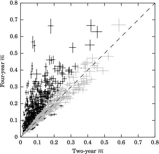
Scatter four-year versus two-year modulation indices for 1134 CGRaBS sources. The dashed line shows the 1:1 relationship for reference. Sources for which the difference in intrinsic modulation index is less than 3σ are plotted in grey.
This systematic increase in the variability index suggests that the two-year interval was insufficiently long to capture the full range of behaviours in many CGRaBS sources: variability on time-scales longer than two years is apparent. This is not surprising. Based on more than 25 years of monitoring at the University of Michigan Radio Astronomy Observatory and the Metsähovi Radio Observatory in Finland, typical flaring time-scales of 4–6 yr were found, sometimes with evidence for changes on time-scales of 10 yr or longer, and typical flare durations of 2.5 yr were reported at 22 and 37 GHz (Hovatta et al. 2007, 2008). Long-time-scale variability is also found in the gamma-ray band. For example, variability on few-year time-scales led to lower ratios between the peak and mean gamma-ray fluxes detected by the LAT during its first 11 months than were found by EGRET during its 4.5 yr lifetime (Abdo et al. 2010b). Thus, as our monitoring programme continues, additional data will likely continue to increase the intrinsic modulation index for some sources. However, the affected sources will be distributed randomly among the subpopulations we use in our studies, so this trend will not create false apparent correlations.
3.2 Outlier contamination
Although our automated data quality filters reject most unreliable observations, our flux density light curves still contain some outlier data points. These are mostly attributable to poor observing conditions or pointing offset measurement failures, and do not represent actual astronomical source variations. These outliers will artificially increase the intrinsic modulation index we compute for an affected source, so we must account for their effect. We cannot simply delete these points from the light curves on the basis that the flux density value differs from neighbouring measurements: blazars are strongly variable objects, and such deletion would bias our results towards our preconception of ‘reasonable’ variability. To avoid such biases, we instead quantify how the presence of outliers affects our calculated intrinsic modulation indices.
The most common extreme outliers are near-zero flux density values reported for normally bright sources. These are probably due to mispointing. High outliers do occur occasionally, though less frequently because they are more effectively removed by our data quality filters. To measure the effect of outliers, we computed the intrinsic modulation indices for each source with the addition of a single ‘false outlier’ flux density value that was twice the average error above zero. High outliers are rarely more than twice the true flux density of a source, so their impact on the intrinsic modulation index is similar to that of the near-zero outliers. We performed this test using modulation indices computed from the first 3.5 years of data for each source. The result is approximately described by a quadrature increase of the intrinsic modulation index by 0.066, as shown in Fig. 2.

Grey points show modulation index data computed with the addition of an extreme outlier data point plotted against the modulation index for the same source calculated from the actual data. The dashed line shows the ideal y = x line. The solid line shows the effect of adding 0.066 in quadrature with the measured modulation index.
We estimate that about 8 per cent of our sources are affected by such outliers (Richards 2012). Because of this low incidence, sources affected by multiple outliers are rare (≲2 per cent). The impact of a second outlier is smaller than that of the first because the intrinsic modulation index is dominated by the largest excursion from the mean. In Richards (2012), addition of a second simulated outlier was found to increase the intrinsic modulation by a mean of only 0.001. We therefore use the effect of a single outlier to estimate the impact on our modulation index results. The incidence of outlier data points should not be correlated with physical properties of the sources, so the net effect of outliers is to increase the average variability of a population, slightly reducing our sensitivity to differences between subpopulations.
3.3 Trends with SED peak frequency
When the intrinsic modulation index is plotted against νpk in Fig. 3, the result appears familiar. Its form strongly resembles equivalent plots of radio core brightness temperatures and fractional polarizations (Lister et al. 2011), gamma-ray variability indices (Ackermann et al. 2011b) and optical intrinsic modulation indices (Hovatta et al. 2013). Fig. 3 differs from these in that there is a rather abrupt decrease in the apparent upper envelope above 1015 Hz, where the others show a smoother transition in the ISP region (for the gamma-ray variability indices and optical modulation indices) or a step decrease at a slightly lower νpk value (nearer to 1014.5 Hz for the radio core brightness temperatures and fractional polarizations). We note that removal of only a few high-|$\overline{m}$|, high-νpk ISP sources would eliminate the abrupt decrease in our plot, so this could be the result of incorrect νpk values. Using the two-sample Kolmogorov–Smirnov test to compare the |$\overline{m}$| values for the three classes, we find that neither the LSP nor the ISP sample is consistent with the null hypothesis of being drawn from the same distribution as the HSP sample (p ≈ 7 × 10⁻⁴ and p ≈ 0.002). For the LSP and ISP samples, we cannot reject the null hypothesis (p ≈ 0.6). As shown in Fig. 4, sources with lower νpk values tend to have higher mean flux densities. This relationship matches that found for parsec-scale 15 GHz flux densities by Lister et al. (2011). Because HSP sources are found at lower flux densities, we measure a value for |$\overline{m}$| for proportionally fewer of these sources. We have not accounted for upper limits in this analysis, but doing so would likely increase the difference between the HSPs and the other classes.
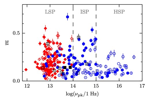
Intrinsic modulation index |$\overline{m}$| versus νpk for the 258 sources in the 1LAC sample with both measured 15 GHz modulation indices in this work and νpk values in Ackermann et al. (2011b). BL Lacs are plotted as blue circles, FSRQs as red diamonds and other classifications as black squares. CGRaBS sources are plotted as filled symbols.
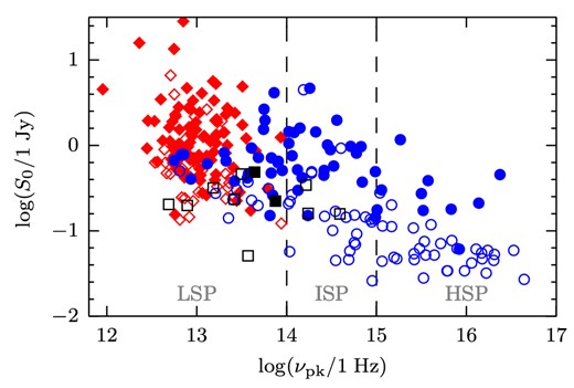
Maximum-likelihood mean flux density, S0 versus νpk for the 248 BL Lacs and FSRQs in the 1LAC sample with both 15 GHz mean flux density values in this work and νpk values in Ackermann et al. (2011b). BL Lacs are plotted as blue circles, FSRQs as red diamonds and other classifications as black squares. CGRaBS sources are plotted as filled symbols.
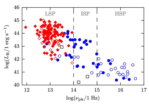
Isotropic radio luminosity, LR versus νpk for the 186 BL Lacs and FSRQs in the 1LAC sample with 15 GHz mean flux density values in this work, known redshifts, and νpk values in Ackermann et al. (2011b). BL Lacs are plotted as blue circles, FSRQs as red diamonds and other classifications as black squares. CGRaBS sources are plotted as filled symbols.
4 POPULATION COMPARISONS
To compare the variability amplitude between source populations in our sample, we apply a likelihood maximization method that requires we specify a parent distribution for the modulation indices. An exponential distribution, |$f(m)=m_{0}^{-1}\exp (-m/m_0)$|, is a qualitatively reasonable fit to the observed distribution of modulation indices in our sample (Richards et al. 2011). This distribution is a monoparametric distribution characterized by its mean, m0. Because of this, numerical integrations are required in only one dimension, making it convenient for our likelihood analyses.
CGRaBS subpopulation intrinsic modulation indices.
| Subpopulation | m0 |
|---|---|
| Gamma-ray loud | |$0.175_{-0.011}^{+0.012}$| |
| Gamma-ray quiet | |$0.099_{-0.003}^{+0.004}$| |
| BL Lac | |$0.163_{-0.014}^{+0.016}$| |
| FSRQ | 0.112 ± 0.004 |
| FSRQ (z < 1) | |$0.123_{-0.007}^{+0.008}$| |
| FSRQ (z ≥ 1) | 0.106 ± 0.005 |
| Subpopulation | m0 |
|---|---|
| Gamma-ray loud | |$0.175_{-0.011}^{+0.012}$| |
| Gamma-ray quiet | |$0.099_{-0.003}^{+0.004}$| |
| BL Lac | |$0.163_{-0.014}^{+0.016}$| |
| FSRQ | 0.112 ± 0.004 |
| FSRQ (z < 1) | |$0.123_{-0.007}^{+0.008}$| |
| FSRQ (z ≥ 1) | 0.106 ± 0.005 |
A source is included in the gamma-ray loud subpopulation if it has a clean association in the 2LAC catalogue (Ackermann et al. 2011b).
1LAC subpopulation intrinsic modulation indices.
| Subpopulation | m0 |
|---|---|
| BL Lac | |$0.150_{-0.014}^{+0.015}$| |
| FSRQ | |$0.181_{-0.013}^{+0.014}$| |
| HSP | |$0.036_{-0.008}^{+0.010}$| |
| ISP | |$0.175_{-0.025}^{+0.031}$| |
| LSP | |$0.177_{-0.013}^{+0.014}$| |
| HSP BL Lac | |$0.036_{-0.008}^{+0.010}$| |
| ISP BL Lac | |$0.178_{-0.026}^{+0.033}$| |
| LSP BL Lac | |$0.155_{-0.027}^{+0.036}$| |
Population variability comparison results.
| Parent pop. | Subpop. A | Subpop. B | Δm0 | Signif. |
|---|---|---|---|---|
| CGRaBS | Gamma-ray loud | Gamma-ray quiet | |$0.075_{-0.012}^{+0.013}$| | 6σ |
| CGRaBS | BL Lac | FSRQ | |$0.050_{-0.015}^{+0.017}$| | 4σ |
| 1LAC | BL Lac | FSRQ | −0.031 ± 0.020 | <2σ |
| BL Lac | CGRaBS | 1LAC | 0.013 ± 0.021 | <1σ |
| FSRQ | CGRaBS | 1LAC | |$-0.068_{-0.015}^{+0.014}$| | 6σ |
| 1LAC | HSP | ISP | |$-0.136_{-0.032}^{+0.027}$| | 5σ |
| 1LAC | HSP | LSP | −0.139 ± 0.017 | 5σ |
| 1LAC | ISP | LSP | |$-0.002_{-0.029}^{+0.033}$| | <1σ |
| 1LAC | HSP BL Lac | ISP BL Lac | |$-0.139_{-0.034}^{+0.028}$| | 4σ |
| 1LAC | HSP BL Lac | LSP BL Lac | |$-0.116_{-0.037}^{+0.029}$| | 4σ |
| 1LAC | ISP BL Lac | LSP BL Lac | |$0.022_{-0.045}^{+0.044}$| | <1σ |
| CGRaBS | FSRQ (z ≥ 1) | FSRQ (z < 1) | −0.018 ± 0.009 | <2σ |
The Δm0 column tabulates the most-likely value of m0, A − m0, B. A source is included in the gamma-ray-loud subpopulation if it has a clean association in the 2LAC catalogue (Ackermann et al. 2011b).
4.1 Gamma-ray loudness
Using our population comparison method, we now investigate whether the connection between gamma-ray emission and radio variability we reported in Richards et al. (2011) persists in our longer data set. We define a CGRaBS source to be gamma-ray loud if it has a ‘clean’ association with a LAT gamma-ray source in the 2LAC catalogue. The likelihood distributions for the gamma-ray-loud and quiet subpopulations are shown in Fig. 6. To evaluate the significance of the separation between the distributions, we compute the likelihood distribution for the difference between the true population means, also shown in Fig. 6. The two distributions are not consistent with each other at the 6σ confidence level with a most-likely difference of 7.5 per cent. As before, gamma-ray-loud sources exhibit higher variability amplitudes than gamma-ray-quiet sources do.
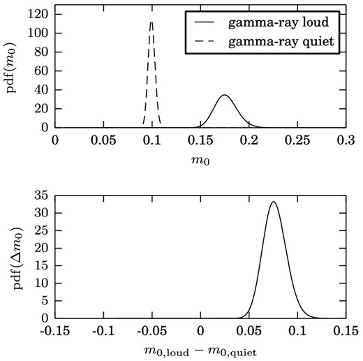
Top: likelihood distributions for m0 for CGRaBS sources that are gamma-ray loud (solid line) and gamma-ray quiet (dashed line). The most-likely value of the mean modulation index for each distribution and for the difference between the two are listed in Tables 3 and 5. A source is considered gamma-ray loud if it is has a clean association in the Fermi 2LAC catalogue (Ackermann et al. 2011b). Bottom: likelihood distribution of the difference between the mean modulation indices. This distribution is inconsistent with a zero mean with about 6σ significance.
4.2 Optical classification
We next examine radio variability amplitude as a function of optical classification, comparing the BL Lac and FSRQ subpopulations. In Fig. 7, we show the likelihood distributions for m0 for sources in the CGRaBS sample. The CGRaBS BL Lacs are found to be more variable at a significance of about 4σ, with a most-likely difference of |$0.050_{-0.015}^{+0.017}$|. This is consistent with the results previously reported for the two-year data set (Richards et al. 2011).
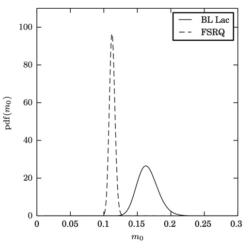
Likelihood distributions for m0 for CGRaBS BL Lacs (solid line) and FSRQs (dashed line). The most-likely values for the mean modulation index for each distribution and for the difference between the two are listed in Tables 3 and 5. The two distributions are not consistent with having the same mean modulation index with about 4σ significance.
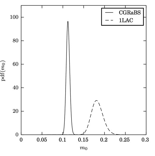
The situation is quite different for the 1LAC sample. Likelihood distributions for m0 for the BL Lac and FSRQ subpopulations of the 1LAC sample are shown in Fig. 8. We find only weak evidence for a difference in m0 between the BL Lac and FSRQ subpopulations (most-likely difference 0.031 ± 0.020, corresponding to <2σ significance). Although the difference is not statistically significant, we note that the mean modulation index for BL Lacs is formally lower than that for FSRQs, while for the CGRaBS sample we find the variability among FSRQs to be significantly higher.
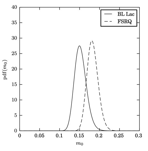
Likelihood distributions for m0 for 1LAC BL Lacs (solid line) and FSRQs (dashed line). The most-likely values for the mean modulation index for each distribution and for the difference between the two are listed in Tables 4 and 5. The two distributions are consistent with having the same mean modulation index at the 2σ level.
As a further test, we compare the variability amplitudes of the CGRaBS and 1LAC samples in Fig. 9 (for BL Lacs) and Fig. 10 (for FSRQs). Note that the individual likelihood distributions shown in Figs 9 and 10 are the same as those in Figs 7 and 8, but are plotted in different pairs. We find no evidence that the BL Lacs in the 1LAC and CGRaBS samples differ in variability amplitude, with a most-likely difference of 0.013 ± 0.021. In contrast, 1LAC FSRQs are more variable than the CGRaBS FSRQs with a most-likely difference of |$0.068_{-0.014}^{+0.015}$|, a difference significant at the 6σ level. Thus, the difference in radio variability between gamma-ray-loud and gamma-ray-quiet CGRaBS blazars reflects a large variability difference between FSRQs in the mostly radio-selected CGRaBS sample and the gamma-ray-selected sample. BL Lacs in either sample exhibit similar radio variability.
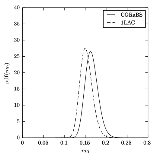
Likelihood distributions for m0 for BL Lacs in CGRaBS (solid line) and 1LAC (dashed line). The most-likely values for the mean modulation index for each distribution and for the difference between the two are listed in Tables 3–5. The two distributions are consistent with having the same mean modulation index at the 1σ level.
Likelihood distributions for m0 for FSRQs in CGRaBS (solid line) and 1LAC (dashed line). The most-likely values for the mean modulation index for each distribution and for the difference between the two are listed in Tables 3–5. The two distributions are not consistent with having the same mean modulation index with about 6σ significance.
4.3 Spectral classification
Comparing the HSP, ISP and LSP populations in the 1LAC sample, we find that the HSP population is less variable than either of the others, while the LSP and ISP populations are not distinguishable. The likelihood distributions are plotted in Fig. 11. The most-likely difference between HSP and LSP populations is 0.139 ± 0.017 and between the HSP and ISP populations is |$0.136_{-0.027}^{+0.032}$|, both significant at about the 5σ level. Between the ISP and LSP populations, the difference is only |$0.002_{-0.033}^{+0.029}$|.
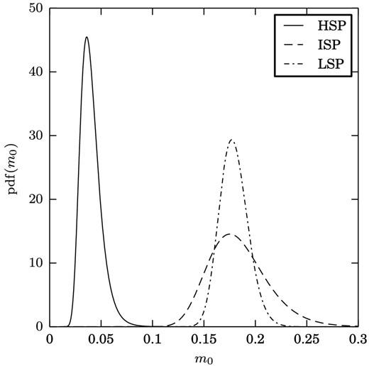
Likelihood distributions for m0 for 1LAC HSP sources (solid line), ISP sources (dashed line), and LSP sources (dot–dashed line). The most-likely values for the mean modulation index for each distribution and for the differences between the pairs are listed in Tables 4 and 5. The ISP and LSP distributions are consistent with having the same mean modulation index at the 1σ level. The HSP distribution is not consistent with either of the others with about 5σ significance.
In Fig. 12, the modulation index likelihood distributions are plotted for the HSP, ISP and LSP BL Lacs in the 1LAC sample.
After excluding the FSRQs, we find essentially the same result as before. The values for the three bins change by less than 1σ, although because the FSRQs are predominantly LSP, the uncertainty for the LSP bin increases substantially due to the reduced number of sources. The HSP population, which is entirely BL Lacs, is less variable than either the ISP or LSP populations at the 4σ level. The ISP and LSP BL Lac populations differ by less than 1σ.
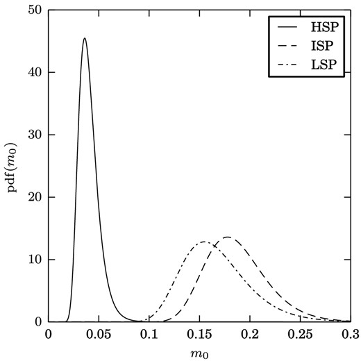
Likelihood distributions for m0 for 1LAC BL Lac sources classified as HSP, (solid line), ISP (dashed line) and LSP (dot–dashed line). The most-likely values for the mean modulation index for each distribution and for the differences between the pairs are listed in Tables 4 and 5. The ISP and LSP distributions are consistent with having the same mean modulation index at the 1σ level. The HSP distribution is not consistent with either of the others with about 4σ significance.
From our 1LAC sample, we measured intrinsic modulation indices for 258 sources that also have νpk values in the 2LAC catalogue (Ackermann et al. 2011b). These are plotted in Fig. 3. BL Lacs and FSRQs clearly occupy different regions of this plot, with FSRQs confined to the left edge but reaching high levels of variability, while BL Lacs are plentiful across the full range of νpk values with only low intrinsic modulation indices at high-νpk values. We note that the sources with the three highest intrinsic modulation indices, J0238+1636, J0654+4514 and J0050−0929, are all highly compact radio sources on parsec scales, which likely indicates that these sources are viewed very nearly along their jet axes (Lister et al. 2009a, 2011, 2013).
4.4 Redshift trend
Based on the two-year results, we found evidence that the intrinsic modulation indices for CGRaBS FSRQs in our sample decreased with increasing redshift (Richards et al. 2011). In Fig. 13, we plot with black circles the mean four-year intrinsic modulation indices among bright (S0 > 400 mJy) CGRaBS FSRQs as a function of redshift. Although the trend suggested by the two-year data, shown here with grey diamonds, remains visible, the scatter of the data within each bin has increased, particularly at higher redshifts. Nonetheless, the correlation is significant (Kendall's τ = −0.15 with p < 5 × 10⁻⁵). This is not due, e.g., to mutual correlation with flux density. We do find a significant correlation between redshift and S0 (τ = −0.15, p < 5 × 10⁻³) but no correlation between S0 and intrinsic modulation index (τ = 0.04, p < 0.48). In Fig. 14, we plot the likelihood distributions for CGRaBS FSRQs at high (z ≥ 1) and low (z < 1) redshift, including those fainter than 400 mJy. Although we continue to find a larger most-likely value of m0 for FSRQs at lower redshift (most-likely difference 0.018 ± 0.009), the significance of the separation is less than 2σ and has fallen slightly compared to the two-year result.
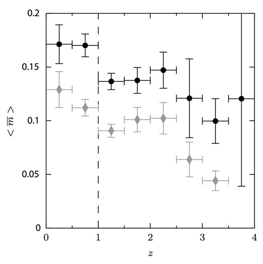
Mean modulation indices for bright (S0 > 400 mJy) CGRaBS FSRQs in redshift bins with Δz = 0.5. Horizontal error bars indicate bin widths, vertical error bars indicate the statistical uncertainty in the plotted means. Black circles indicate data points computed from the four-year data set, grey diamonds from the two-year data set. The vertical dashed line indicates z = 1.
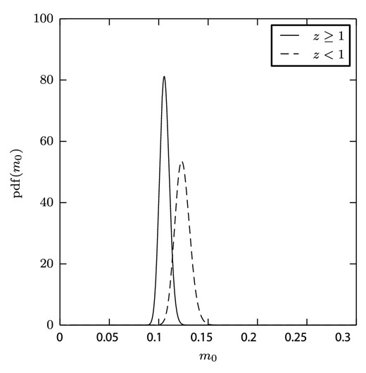
Likelihood distributions for m0 for the CGRaBS FSRQs with known redshift in our monitoring sample with z ≥ 1 (solid line) and z < 1 (dashed line). The most-likely values for the mean modulation index for each distribution and for the difference between the two are listed in Tables 3 and 5. The two distributions are consistent with having the same mean modulation index at the 2σ level.
As discussed in Richards et al. (2011), there are several competing effects that will contribute to such a trend. Due to cosmological time dilation, equal-length observations will correspond to different source-frame time intervals according to Δtsource = (1 + z)−1Δtobs. Because, as we showed in Section 3.1, the intrinsic modulation index increases with the observation length, this will tend to decrease |$\overline{m}$| with increasing redshift. This effect explains at least part of our observed redshift trend. Richards (2012) used a subset of the OVRO data set to investigate this effect by comparing the variability in equal rest-frame time periods. Accounting for this reduced the most-likely difference between the z ≥ 1 and z < 1 samples slightly, although the change was within the uncertainty.
At higher redshifts, the 15 GHz observed frequency corresponds to a higher rest-frame emission frequency. Although blazar variability indices do not differ significantly between 8 and 90 GHz, the source-frame characteristic time between blazar flares at 15 GHz is somewhat longer than at 37 GHz (Hovatta et al. 2007, 2008). Thus, lower redshift blazars will likely have undergone fewer flares in a given source-frame time period. This will tend to reduce the observed intrinsic modulation index, particularly before the source's range of behaviour has been completely measured. The overall increase in intrinsic modulation indices between the two- and four-year data sets, illustrated in Fig. 1, suggests that we have not yet achieved this. This will tend to increase the intrinsic modulation index with redshift, in opposition to our detected trend.
Other effects, such as Doppler and Malmquist biases will also contribute to the redshift trend (Lister & Marscher 1997). Determining whether an intrinsic component to this apparent evolution is present will require Monte Carlo simulation to assess the net contributions of the various biases.
5 DISCUSSION
We have presented and examined the results of four years of twice-weekly 15 GHz radio monitoring of more than 1400 blazars, including systematically radio- and gamma-ray-selected samples. Using the intrinsic modulation index to quantify the variability amplitude for each source, we find that on average, gamma-ray-loud CGRaBS sources are significantly more radio variable than gamma-ray-quiet CGRaBS sources, confirming our previous result (Richards et al. 2011). This reflects a significant difference in variability between FSRQs in the radio-selected CGRaBS and gamma-ray-selected 1LAC samples. This indicates that among FSRQs, there is clearly a connection between gamma-ray emission and radio variability. The 1LAC sample contains primarily strongly radio-variable FSRQs. The CGRaBS sample also contains many FSRQs that are both gamma-ray-loud and strongly radio variable, but it also contains a substantial gamma-ray-quiet, weakly radio-variable FSRQ population. BL Lacs show similar radio variability in both the gamma-ray- and radio-selected samples.
Within the 1LAC sample, the radio variability amplitude is connected to the frequency of the synchrotron SED peak, νpk. HSP blazars, with νpk > 1015 Hz, show significantly less radio variability than do either ISP or LSP blazars. This result persists when FSRQs are excluded and only BL Lacs are considered. In fact, the variability of both the ISP and LSP BL Lacs is the same as that of FSRQs to the 1σ level. This agrees with and quantifies a previous report that HSP BL Lacs tend to have moderately low-modulation indices in the OVRO 15 GHz data, while many LSP and ISP sources vary at higher levels (Lister et al. 2011). We do not find evidence for a difference in radio variability amplitude between the ISP and LSP blazars, and among BL Lacs find a slightly lower level of variability among LSPs, although the uncertainties are relatively large and the difference is less than 1σ.
Hovatta et al. (2013) examined blazar optical variability and found a monotonic increase from HSP to ISP to LSP sources. A continuous trend in gamma-ray variability index versus νpk was also found by Ackermann et al. (2011b). The ability to detect such a trend in these bands benefits from the substantially stronger variability there than at 15 GHz. In gamma-rays in particular, sources are typically undetected when quiescent, whereas the presence of extended radio emission provides a steady background that dilutes the fractional variability measured by the intrinsic modulation index. We find that the steady flux density background increases at lower νpk values. If there is an upper limit to the component of the flux densities that is variable on the week-to-year time-scales we probe with this programme, this would lead to a saturation effect: as the steady flux density increases, the intrinsic modulation index corresponding to the maximum variable flux density will decrease. A limit on the variable flux density is likely because we expect limits on intrinsic brightness temperatures (Kellermann & Pauliny-Toth 1969; Readhead 1994).
These results suggest that, among FSRQs, there is a connection between detectable gamma-ray emission and radio variability. No evidence for such a connection is found for BL Lacs. This finding is similar to the results of several other recent radio blazar studies. Compared to their gamma-ray-quiet counterparts, LAT-detected gamma-ray-loud FSRQs have been found to exhibit faster parsec-scale jet speeds (Lister et al. 2009b) and larger core brightness temperatures, incidence of polarization and parsec-scale opening angles (Linford et al. 2011, 2012a). In most cases, no significant difference has been found between gamma-ray-loud and gamma-ray-quiet BL Lac populations. Linford et al. (2011) did report gamma-ray-loud BL Lacs to have longer jet lengths and Linford et al. (2012a) found they had a slightly higher incidence of core polarization.
The presence of this connection in FSRQs and its apparent absence in BL Lacs may result from different sources of inverse Compton seed photons in these classes. High-energy photons produced by the EC process are beamed more strongly compared to photons produced by either the synchrotron or SSC processes (Dermer 1995), so for a single Lorentz-factor jet, gamma rays produced via EC will be emitted into a smaller solid angle than SSC gamma rays. Several studies have found evidence that BL Lac sources are typically dominated by the SSC process while FSRQs chiefly emit via the EC process (e.g. Abdo et al. 2010c; Lister et al. 2011), and it seems that more powerful jets like those found in FSRQs are more likely to exhibit EC (Meyer et al. 2012). There do, however, seem to be exceptions to this rule (e.g. Boettcher 2012). Still, if this connection is generally correct, then the gamma-ray-loud subset of FSRQs would consist of those whose line of sight falls within the narrow gamma-ray emission cone, which would be the higher Doppler factor sources. Higher Doppler factors are associated with increased radio variability (e.g. Lähteenmäki & Valtaoja 1999; Jorstad et al. 2001a; Hovatta et al. 2009), so this would lead to gamma-ray-loud FSRQs being more radio variable than the overall average, as we find. In BL Lacs, on the other hand, SSC gamma-ray emission would be subject to the same beaming factor as the radio emission, so this selection bias towards higher Doppler factors will be weaker or absent. The population of BL Lacs that exhibit substantial gamma-ray emission would primarily be determined by factors other than beaming effects, as suggested by Lister et al. (2009b).
We caution, however, that we may be overinterpreting our BL Lac result: a selection effect may bias our variability average for this class. The CGRaBS and 1LAC BL Lac samples differ strongly in the proportion of HSP sources in each. Although we do not have uniform SED classifications for the CGRaBS sample, of the 60 that do have classifications only 11 are HSP. For 1LAC, 85 of the 168 with classifications are HSP. Since HSP BL Lacs are much less variable than either ISP or LSP BL Lacs, it is surprising that we find overall similar intrinsic modulation indices for the CGRaBS and 1LAC BL Lac samples. This happens because HSP sources are fainter and less variable in radio, and so are more likely to be dropped by our cuts in S0 and |$\overline{m}$|. As a result, HSP BL Lacs are under-represented in the determination of the mean intrinsic modulation index for the 1LAC sample, leading to an overestimate of m0.
Finally, the observed trend of decreasing variability amplitude with increasing redshift among CGRaBS FSRQs appears still to be present in our longer data sets, albeit with reduced significance when we compare the mean intrinsic modulation indices of high- and low-redshift objects. The correlation between |$\overline{m}$| and z for bright FSRQs is highly significant (p < 5 × 10⁻⁵), however. There are several effects and biases that will contribute to such a trend, so determining whether a cosmological evolution component is present will likely require simulations.
JLR would like to thank Matthew L. Lister for several helpful discussions. The OVRO 40 m monitoring programme is supported in part by National Science Foundation (NSF) grants AST-0808050 and AST-1109911 and NASA grants NNX08AW31G and NNX11AO43G. TH was supported by the Jenny and Antti Wihuri foundation. VP acknowledges support from the ‘RoboPol’ project, which is implemented under the ‘Aristeia’ Action of the ‘Operational Programme Education and Lifelong Learning’ and is co-funded by the European Social Fund (ESF) and Greek National Resources; and from the European Commission Seventh Framework Programme (FP7) through grants PCIG10-GA-2011-304001 ‘JetPop’ and PIRSES-GA-2012-31578 ‘EuroCal.’ The National Radio Astronomy Observatory is a facility of the National Science Foundation operated under cooperative agreement by Associated Universities, Inc. This research has made use of the NASA/IPAC Extragalactic Database (NED) which is operated by the Jet Propulsion Laboratory, California Institute of Technology, under contract with the National Aeronautics and Space Administration.
These percentages do not sum to exactly 100 per cent due to rounding.
REFERENCES
SUPPORTING INFORMATION
Additional Supporting Information may be found in the online version of this article:
Table 1. Source properties and results.
Table 2. 15 GHz light-curve data (Supplementary Data).
Please note: Oxford University Press are not responsible for the content or functionality of any supporting materials supplied by the authors. Any queries (other than missing material) should be directed to the corresponding author for the article.
