X-ray detections of submillimetre galaxies: active galactic nuclei versus starburst contribution

Johnson, S. P.; Wilson, G. W.; Wang, Q. D.; Williams, C. C.; Scott, K. S.; Yun, M. S.; Pope, A.; Lowenthal, J.; Aretxaga, I.; Hughes, D.; Kim, M. J.; Kim, S.; Tamura, Y.; Kohno, K.; Ezawa, H.; Kawabe, R.; Oshima, T.

doi:10.1093/mnras/stt197

Abstract

We present a large-scale study of the X-ray properties and near-IR-to-radio spectral energy distributions (SEDs) of submillimetre galaxies (SMGs) detected at 1.1 mm with the AzTEC instrument across a ∼1.2 square degree area of the sky. Combining deep 2–4 Ms Chandra data with Spitzer IRAC/MIPS and Very Large Array data within the Great Observatories Origins Deep Survey North (GOODS-N), GOODS-S and COSMOS fields, we find evidence for active galactic nucleus (AGN) activity in ∼14 per cent of 271 AzTEC SMGs, ∼28 per cent considering only the two GOODS fields. Through X-ray spectral modelling and multiwavelength SED fitting using Monte Carlo Markov chain techniques to Siebenmorgen et al. (AGN) and Efstathiou, Rowan-Robinson & Siebenmorgen (starburst) templates, we find that while star formation dominates the IR emission, with star formation rates (SFRs) ∼100–1000 M_⊙ yr⁻¹, the X-ray emission for most sources is almost exclusively from obscured AGNs, with column densities in excess of 10²³ cm⁻². Only for ∼6 per cent of our sources do we find an X-ray-derived SFR consistent with NIR-to-radio SED derived SFRs. Inclusion of the X-ray luminosities as a prior to the NIR-to-radio SED effectively sets the AGN luminosity and SFR, preventing significant contribution from the AGN template. Our SED modelling further shows that the AGN and starburst templates typically lack the required 1.1 mm emission necessary to match observations, arguing for an extended, cool dust component. The cross-correlation function between the full samples of X-ray sources and SMGs in these fields does not indicate a strong correlation between the two populations at large scales, suggesting that SMGs and AGNs do not necessarily trace the same underlying large-scale structure. Combined with the remaining X-ray-dim SMGs, this suggests that sub-mm-bright sources may evolve along multiple tracks, with X-ray-detected SMGs representing transitionary objects between periods of high star formation and AGN activity, while X-ray-faint SMGs represent a brief starburst phase of more normal galaxies.

galaxies: active, galaxies: high-redshift, galaxies: starburst, submillimetre: galaxies, X-rays: galaxies

INTRODUCTION

Large blank-field surveys made at (sub-)millimetre wavelengths have identified a large population of bright, high-redshift galaxies (e.g. Hughes et al. 1998; Coppin et al. 2006; Bertoldi et al. 2007; Perera et al. 2008; Weiß et al. 2009; Scott et al. 2010, and references therein). These submillimetre galaxies (SMGs) are characterized by high infrared (IR) luminosities, ≳10¹² L_⊙ (Blain et al. 2004; Chapman et al. 2005) and a redshift distribution peaking around z ∼ 2 (Chapman et al. 2005). SMGs are therefore believed to be the high-redshift analogues to local ultraluminous IR galaxies (ULIRGs) and are possible progenitors of today's massive ellipticals (e.g. Smail et al. 2004; Chapman et al. 2005). However, SMGs at z ∼ 2 are more numerous than local ULIRGS by several orders of magnitude and likely dominate the total IR luminosity density at z ∼ 2 (Le Floc'h et al. 2005; Pérez-González et al. 2005; Hopkins et al. 2010). The origin of these luminous, high-redshift sources is still under debate due, in part, to the low angular resolution at (sub-)millimetre wavelengths of current instruments and the relative faintness of likely counterparts. Multiwavelength and IR spectroscopic follow-up studies of SMGs using Spitzer (see, for example, Menéndez-Delmestre et al. 2007; Nardini et al. 2008; Pope et al. 2008) suggest that SMGs are largely dust-obscured starburst (SB) systems with star formation rates (SFRs) ∼1000 M_⊙ yr⁻¹. However, it is becoming increasingly apparent through the high X-ray detection rate of SMGs (∼30–50 per cent; see Alexander et al. 2005a,b; Laird et al. 2010; Georgantopoulos, Rovilos & Comastri 2011) and SMG case studies (i.e. Tamura et al. 2010) that emission from active galactic nuclei (AGNs) may also be a crucial component to the energetic output of SMGs.

The likely connection between SB and AGN activity in SMGs is further supported by the concurrent nature of the cosmic SFR and black hole accretion with peaks at z ∼ 2 (e.g., Merloni 2004; Le Floc'h et al. 2005). Simulations of SMG formation in a merger-driven scenario also suggest that the SMG phase precedes rapid growth of a central AGN (Narayanan et al. 2010). SMGs may therefore represent an important phase in galaxy evolution and may shed light on the origin of observed relations between AGN activity and stellar mass in local galaxies (i.e. the M-σ relation; Ferrarese & Merritt 2000; Gebhardt et al. 2009; Gultekin et al. 2009). One should be cautious, however, in extrapolating the SB–AGN connection to the most extreme objects (i.e. radio-loud AGN; Dicken et al. 2012, and references therein) though such cases are a fundamentally different population of sources. Unfortunately, while there are a multitude of methods for studying AGN and star formation, disentangling their relative contributions to a galaxy's bolometric output remains challenging. Obtaining redshifts and other information via optical/ultraviolet imaging and spectroscopy is exceptionally difficult as SMGs are both distant and optically thick (see the review by Blain et al. 2002). IR spectroscopy of SMGs typically shows strong polycyclic aromatic hydrocarbon (PAH) features associated with star-forming regions, although there are cases of power-law-like spectra indicative of AGN (Menéndez-Delmestre et al. 2007; Coppin et al. 2008; Nardini et al. 2008; Pope et al. 2008). Arguably, the best indicator for AGN activity is hard X-rays (>2 keV), which penetrate obscuring dust up to the Compton-thick limit (neutral hydrogen column densities of N_H ≳ 10²⁴ cm⁻²). X-ray detections are not uniquely attributable to AGN, however, as high SFRs may produce numerous high-mass X-ray binaries (HMXBs) that mimic the emission of low-luminosity AGNs.

In the past decade there have been a few studies that consider X-ray counterparts to SMGs for evidence of AGN activity, though this number has expanded in recent years. Alexander et al. (2005a,b, hereafter A05a,b) provide the earliest analysis by examining the Chandra counterparts to SCUBA (Holland et al. 1999) 850 μm identified sources in the Great Observatories Origins Deep Survey (GOODS) North field. In their sample of 20 SMGs with radio and spectroscopic redshift identifications taken from Chapman et al. (2005), they find that ∼75 per cent have X-ray properties consistent with obscured (N_H ≳ 10²³ cm⁻²) AGN activity. Accounting for SMGs without spectroscopic redshifts, they suggest that the true X-ray detection rate may be significantly lower, ≳28 per cent. However, the A05a,b sample may contain biases introduced through the Chapman et al. (2005) SCUBA source catalogue, which consists of observations of known radio sources and low signal-to-noise (S/N < 3.5σ) sources and thus may not be representative of the entire bright SMG population (see also Younger et al. 2007). Further X-ray/SMG counterpart analysis has been provided by Laird et al. (2010, hereafter LNPS10), who find an ∼45 per cent X-ray detection rate to radio and/or Spitzer-identified SCUBA sources (Pope et al. 2006) with an ∼20–29 per cent AGN identification rate based on X-ray spectral modelling. LNPS10 find that the bolometric far-infrared (FIR) emission is dominated by star formation in the majority of their sources (∼85 per cent) after including available Spitzer photometry, consistent with A05a,b and other IR studies of SMGs (i.e. Menéndez-Delmestre et al. 2007, 2009; Valiante et al. 2007).

More recently, the studies of Georgantopoulos et al. (2011, hereafter GRC11), Hill & Shanks (2011) and Bielby et al. (2012) have utilized LABOCA data in the Extended Chandra Deep Field South (ECDFS; Weiß et al. 2009) and William Herschel Deep Field. The analysis of GRC11 is similar to that of LNPS10 who also find an AGN fraction of <26 ± 9 per cent with the mid-IR emission dominated by SB activity, though the fraction of SB-powered X-ray sources is lower than estimated by LNPS10. The works of Hill & Shanks (2011) and Bielby et al. (2012) consider a more statistical approach, utilizing the full catalogues rather than individual sources as in A05a,b, LNPS10 and GRC11, though find a similar SMG/X-ray detection rate (∼20 per cent). They also find that obscured AGNs preferentially have greater sub-mm emission than unobscured AGNs, a result confirmed through EVLA observations by Heywood et al. (2012). Lutz et al. (2010) find a similar relation in the ECDFS where the X-ray luminosity and absorbing column density for bright AGNs, L_2-10 keV ≳ 10⁴³ erg s^{− 1}, are correlated with the 870 μm flux, implying a close connection to star formation. This assumes, however, that the X-ray emission is purely from the AGN while the 870 μm flux is only from star formation. Furthermore, the Lutz et al. (2010) study does not account for X-ray-bright SMGs, which may potentially bias the stacking results.

To recap, X-ray studies to date find that the AGN fraction of SMGs is in the range of ∼20–45 per cent and that the bolometric IR luminosity of SMGs is dominated by SBs.

In this work, we examine the identification rate and contribution of AGNs to the emission at various wavelength regimes in AzTEC SMGs. Our sample consists of Chandra X-ray counterparts to AzTEC 1.1 mm sources found in the GOODS-North, GOODS-South and COSMOS fields, providing a total Chandra sky coverage of ∼1.15 square degrees (∼0.12, ∼0.11 and ∼0.92 square degrees, respectively) with more than 2600 identified X-ray sources. This large sample size will reduce any biases due to cosmic variance in previous studies. Furthermore, we do not base our sample selection and counterpart identification on prior source association, thus removing any possible pre-identification bias. The available multiwavelength photometry in these fields, including Spitzer IRAC and MIPS, will provide additional constraints on the AGN identification rate and contribution to the bolometric output of our sources.

We begin with a description of the AzTEC and Chandra data and reduction procedures. We then detail our method for identifying X-ray counterparts to the AzTEC sources and subsequent multiwavelength counterparts. Our analysis of the X-ray-identified AzTEC sources follows a two-pronged approach: (1) applying X-ray spectral models and spectral energy distribution (SED) templates to the X-ray spectra and near-IR-to-radio SED, which will provide the basic information concerning the contribution of AGN and star formation in each wavelength regime; and (2) linking the X-ray spectral fits to the near-IR-to-radio SED modelling, thus providing a greater insight into the AGN/star formation connection. Our SED fitting differs from typical SED analyses (e.g. Serjeant et al. 2010) in that we employ a Monte Carlo Markov chain (MCMC) technique. We close by comparing the implications of our work to those of previous X-ray/SMG results in addition to the X-ray/SMG cross-correlation relation. Additional analysis of our data, including source stacking and IR-optical-UV fitting, will be presented in future publications.

Throughout this work, we assume a flat Λ cold dark matter cosmology with H₀ = 70 km s^{− 1} Mpc^{− 1}, Λ₀ = 0.73 and Ω_M = 0.27.

OBSERVATIONS AND DATA PROCESSING

AzTEC: 1.1 mm observations

AzTEC (Wilson et al. 2008) is a 144-element bolometer array operating at 1.1 mm and installed on the 50 m Large Millimetre Telescope (LMT; Schloerb 2008). Prior to its installation on the LMT, AzTEC has performed several science observations on the James Clerk Maxwell Telescope (JCMT) and the Atacama Submillimeter Telescope Experiment (ASTE), including blank fields (namely GOODS-N, GOODS-S and COSMOS) and high-redshift radio clusters. Here, we briefly describe the AzTEC observations and 1.1 mm source sample that will be used in our analysis.

During the JCMT 2005 and 2006 observing campaign, Perera et al. (2008) imaged a 21 arcmin × 15 arcmin area of the GOODS-N region. During the 2007 and 2008 observation seasons on ASTE, AzTEC imaged both GOODS-S (Scott et al. 2010) and the 1 square degree area of COSMOS (Aretxaga et al. 2011). In reducing the raw time streams for each set of observations, an iterative technique using the principal component analysis (PCA) is used to filter out the atmospheric signal that dominates the raw observed data. Downes et al. (2012) provide a discussion on correcting the PCA transfer function and list revised catalogues for previously released AzTEC data. Here, we use the revised catalogues of Downes et al. for GOODS-N and GOODS-S; the COSMOS catalogue of Aretxaga et al. (2011) follows this prescription. The final AzTEC maps are constructed to have uniform coverage and sensitivity, providing a 1σ rms of ∼1.3 mJy in GOODS-N and COSMOS. The GOODS-S map reaches the confusion limit of AzTEC on ASTE for a depth of (1σ rms) ∼0.6 mJy. Sources are defined as peaks in the signal map with S/N ≥ 3.5σ, resulting in a total sample of 277 AzTEC sources (40, 48 and 189 in GOODS-N, GOODS-S and COSMOS, respectively) where ≲20 are expected to be false detections. Note, however, that the false detection rate is estimated for an S/N threshold of ∼3.5σ and decreases rapidly for higher source S/N. For the following analysis, we use the full sample of 277 AzTEC sources, applying no additional source-selection criteria.

Chandra observations

The Chandra X-ray Observatory provides deep observations of the GOODS-N, GOODS-S and COSMOS fields (for details on the observations, see Alexander et al. 2003; Luo et al. 2008; Elvis et al. 2009, respectively) with a total exposure time of ∼2 Ms in each field. More recently, an additional ∼2 Ms has been added to GOODS-S with 31 additional pointings, bringing the final integrated exposure time to ∼4 Ms (Xue et al. 2011). Due to the pointing strategy for COSMOS, effective exposures only reach ∼200 ks for the inner ∼0.5 square degrees (see also Elvis et al. 2009). As a result, the X-ray photon statistics in COSMOS are very poor, leading to weak constraints on the X-ray spectral properties (Section 3.1). This is somewhat offset by its larger area than the GOODS fields by allowing for more potential counterparts (Section 2.3). On the other hand, the deep 4 Ms data in GOODS-S provide the greatest improvement to the counting statistics, and thus spectral modelling, to date, a valuable asset for potentially faint and highly obscured AGNs. All of the fields were imaged with the Advanced CCD Imaging Spectrometer Imaging array, which is composed of four CCDs arranged in a 2 × 2 grid that operate together to provide an ∼17 arcmin × 17 arcmin field of view with sub-arcsecond resolution at the telescope aimpoint, degrading with increasing off-axis distance.

To ensure uniformity in our analysis, all observations were re-reduced using Chandra Interactive Analysis of Observations (ciao version 3.4) routines and custom routines developed for working with merged X-ray data sets; using the published X-ray catalogues of Alexander et al. (2003), Luo et al. (2008), Xue et al. (2011) and Elvis et al. (2009) would have required additional calibrations for compatibility. Event files and exposure maps constructed in the 0.5–8.0 keV energy range were made for all observations and then merged to produce final maps for the three fields.

We use the source detection method of Wang (2004), with a false detection probability threshold of 10⁻⁶, to produce X-ray source lists from the final images for cross-correlation with the AzTEC sample and spectral extraction. This detection method uses a wavelet analysis of the input images (in this case, the final merged X-ray images for each field) followed by a sliding-box map detection and maximum likelihood analysis for both source centroiding and optimal photometry. During the source detection, the X-ray maps are divided into different energy bands (i.e. 0.5–8.0 keV full band, 0.5–2.0 keV soft band and 2.0–8.0 keV hard band), resulting in a source catalogue that includes all sources found in each energy band along with their respective count rates and positional uncertainties. The source detection process also produces a list of source regions, which are defined as circular regions with radius equal to twice the 90 per cent energy encircled fraction [defined according to the point spread function (PSF) at the source position].

COSMOS poses a dilemma for source detection due to the blending of PSFs from the tiling of observations. To avoid this issue, we perform the X-ray source detection on the individual observations and then combine the resulting source lists into a final catalogue. Derived parameters are re-calculated for each source using the final COSMOS map, with extraction radii determined from the smallest PSF corresponding to each source. Alternatively, one could simply average the subcatalogues to produce the final catalogue; however, this may exclude X-ray counts present in an image where the source was not initially detected. Certainly, this method has difficulty in detecting the faintest sources present in COSMOS; nevertheless, this will not significantly influence our results given the already low depth of COSMOS compared to the two GOODS fields.

Combining the source lists from each field results in a total of 2630 X-ray sources available for our study. Individually, there are 478, 526 and 1626 sources in GOODS-N, GOODS-S and COSMOS, respectively. Despite the differences in data reduction and source detection, our source lists recover ≳90 per cent of those from the published catalogues of Alexander et al. (2003), Luo et al. (2008), Xue et al. (2011) and Elvis et al. (2009). However, we miss many faint sources from the published catalogues due to our more stringent false detection threshold of 10⁻⁶ versus ∼1–2 × 10⁻⁵ for the other catalogues.

Counterpart candidates

Chandra counterparts

The beam size of AzTEC on the JCMT and ASTE is 18 and 28 arcsec full width at half-maximum, respectively, making reliable X-ray counterpart identification challenging. Following the method of Chapin et al. (2009), we use a fixed search radius of 6 arcsec in GOODS-N and 10 arcsec in GOODS-S and COSMOS to find potential counterparts to the AzTEC sources. Our choice of 10 arcsec in GOODS-S and COSMOS is consistent with a derived search radius for a source with S/N ∼ 5.5 on the ASTE telescope according to Ivison et al. (2007) and roughly corresponds to the average search radius for the AzTEC GOODS-S catalogue (Scott et al. 2010). Simulations in each field agree well with the Ivison et al. (2007) estimate and show that sources with S/N ≳ 3.5 are recovered within the respective search radii >85 per cent of the time. Extending the search radius beyond our adopted value increases the number of X-ray counterparts; however, these additional X-ray sources are unlikely to be true counterparts (see below).

As shown in Fig. 1, there is significant overlap between the AzTEC and Chandra maps. Considering only the overlapping regions, our sample is limited to 271 (39, 47 and 185 in GOODS-N, GOODS-S and COSMOS, respectively) of the initial 277 AzTEC sources and 2229 (397, 429 and 1403, respectively) of the 2630 Chandra sources. Of the remaining 271 AzTEC sources, we find 38 with at least 1 X-ray counterpart (8, 16 and 14 for GOODS-N, GOODS-S and COSMOS, respectively); 5 have 2 potential counterparts and 1 has 3. For those sources with multiple potential Chandra counterparts, we treat each source individually and do not attempt to split the AzTEC flux as we have no prior information on how it may be related to the potential X-ray sources. Overlapping spectral regions for these sources is not an issue as the uncertainty in the X-ray spectra is dominated by the low counting statistics. There are a total of 45 X-ray sources associated with the AzTEC sample, of which only 2 to 3 are expected to be false identifications due to random alignments. Comparatively, the expected number of X-ray pairs for the entire sample of 271 AzTEC sources, assuming a purely random X-ray source population, is ∼14. The AzTEC/X-ray identification rate is therefore ∼14 per cent, lower than estimates reported by A05a and LNPS10 due to the shallower X-ray depth of the COSMOS field; removing it increases the identification rate to ∼28 per cent.

Figure 1.

Open in new tab Download slide

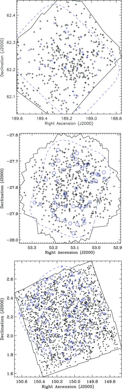
Chandra (solid black line) and AzTEC (dashed blue line) coverage regions for GOODS-N (upper), GOODS-S (middle) and COSMOS (lower). The AzTEC coverage given here corresponds to the 50 per cent uniform coverage region used for source detection. The small circles with radii equal to the AzTEC beam size (18 arcsec in GOODS-N and 28 arcsec in GOODS-S and COSMOS) are plotted at the AzTEC source positions. X-ray source positions are indicated by the small ‘plus’ symbols.

To assess the robustness of our X-ray counterpart identifications, we compute the probability P of random association for a given AzTEC/X-ray pair given the search radii and X-ray source densities (2.97, 3.14 and 1.39 × 10⁻⁴ arcsec⁻² for GOODS-N, GOODS-S and COSMOS, respectively) using the method of Downes et al. (1986), which corrects for the use of a finite search radius and flux-limited source density. The majority of the AzTEC/X-ray pairs (32/45) have P ≤ 0.05 which we define as a ‘robust’ counterpart, the remaining AzTEC/X-ray pairs, with P = 0.05–0.10, are ‘tentative’ associations. Table 1 provides the list of the Chandra-detected AzTEC sources along with their relevant source properties and P values.

Table 1.

Chandra identifications of AzTEC sources in GOODS-N, GOODS-S and COSMOS. Errors are given at the 1σ confidence level. Column 1: AzTEC source ID prefixed by field (i.e. AzGN24 for source 24 in the AzTEC GOODS-N catalogue). Column 2: Chandra ID following IAU standards. Column 3: positional offset between AzTEC and Chandra sources. Errors are derived from Chandra positional uncertainty. Column 4: Chandra 0.5–8.0 keV full band count rate. Column 5: total counts within the source regions as defined from our X-ray source detection. Column 6: estimated background counts within the source regions. Column 7: deboosted AzTEC source flux (see section 3.5 of Austermann et al. 2010 and section 6.2 of Scott et al. 2010). Column (8): probability P of the Chandra source being a random association.

SMM ID	Chandra coordinate	δ_x	0.5–8.0 keV count rate	Source counts	Background counts	1.1 mm flux	P
	(J2000)	(arcsec)	(counts ks⁻¹)			(mJy)
(1)	(2)	(3)	(4)	(5)	(6)
AzGN24	J123608.57+621435.8^a	5.4±0.8	0.031 ± 0.007	98	61	3.1 ± 1.3	0.03
AzGN16a	J123615.83+621515.9^a	3.1 ± 0.5	0.067 ± 0.008	223	42	3.6 ± 1.3	0.03
AzGN16b	J123615.93+621522.0	4.6 ± 0.9	0.013 ± 0.005	51	49	3.6 ± 1.3	0.02
AzGN16c	J123616.08+621514.1^a	3.7 ± 0.4	0.089 ± 0.009	184	46	3.6 ± 1.3	0.02
AzGN10	J123627.52+621218.3	2.7 ± 0.5	0.043 ± 0.007	95	42	4.5 ± 1.3	0.02
AzGN11	J123635.86+620707.8	1.8 ± 2.7	0.176 ± 0.017	812	565	4.1 ± 1.3	0.01
AzGN14	J123651.70+621221.7	4.4 ± 0.4	0.222 ± 0.015	301	42	3.7 ± 1.3	0.03
AzGN7a	J123711.32+621331.1^a	3.3 ± 1.0	0.047 ± 0.008	173	106	5.3 ± 1.3	0.02
AzGN7b	J123711.98+621325.8^a	4.5 ± 1.1	0.043 ± 0.008	150	100	5.3 ± 1.3	0.03
AzGN26	J123713.84+621826.2^a	0.5 ± 1.5	0.195 ± 0.016	486	262	2.8 ± 1.4	0.001
AzGN23	J123716.63+621733.4	2.3 ± 1.3	2.101 ± 0.045	2789	218	3.1 ± 1.3	0.01
AzGS29	J033158.25−274458.8	9.6 ± 2.9	0.079 ± 0.013	1865	1542	2.3 ± 0.6	0.09
AzGS8a	J033204.48−274643.3	8.7 ± 1.5	0.201 ± 0.012	1111	650	3.4 ± 0.6	0.09
AzGS8b	J033205.34−274644.0	2.8 ± 1.4	0.150 ± 0.010	917	591	3.4 ± 0.6	0.03
AzGS10	J033207.12−275128.6	2.9 ± 2.2	0.020 ± 0.008	715	703	3.8 ± 0.7	0.03
AzGS38a	J033209.26−274240.9	3.7 ± 2.7	0.078 ± 0.011	1923	1206	1.7 ± 0.6	0.04
AzGS38b	J033209.71−274249.0	8.0 ± 2.2	0.138 ± 0.013	1705	1106	1.7 ± 0.6	0.09
AzGS1	J033211.39−275213.7	3.2 ± 1.4	0.774 ± 0.021	2338	609	6.7 ± 0.6	0.03
AzGS13	J033212.23−274620.9	5.7 ± 0.8	0.247 ± 0.012	789	260	3.1 ± 0.6	0.07
AzGS7	J033213.88−275600.2	8.7 ± 3.4	0.189 ± 0.019	1932	1497	3.8 ± 0.6	0.09
AzGS11	J033215.32−275037.6	6.6 ± 0.8	0.065 ± 0.007	378	236	3.3 ± 0.6	0.08
AzGS17a	J033222.17−274811.6	6.6 ± 0.3	0.059 ± 0.006	176	52	2.9 ± 0.6	0.08
AzGS17b	J033222.56−274815.0	1.6 ± 0.5	0.029 ± 0.004	123	53	2.9 ± 0.6	0.01
AzGS34	J033229.46−274322.0	9.8 ± 1.4	0.027 ± 0.006	492	392	1.7 ± 0.6	0.09
AzGS20	J033234.78−275534.0	4.8 ± 2.6	0.108 ± 0.013	1853	1490	2.7 ± 0.6	0.05
AzGS14	J033235.18−275215.7	9.2 ± 1.0	0.034 ± 0.006	381	295	2.9 ± 0.6	0.09
AzGS16	J033238.01−274401.2	6.3 ± 1.6	0.012 ± 0.006	392	344	2.7 ± 0.6	0.07
AzGS18	J033244.02−274635.9	5.7 ± 0.6	0.188 ± 0.011	592	198	3.1 ± 0.6	0.07
AzGS25	J033246.83−275120.9	6.9 ± 1.3	0.041 ± 0.007	521	400	1.9 ± 0.6	0.08
AzGS9	J033302.94−275146.9	5.1 ± 3.1	0.204 ± 0.020	1421	1097	3.6 ± 0.6	0.06
AzC56	J095905.05+022156.4	2.7 ± 2.6	0.087 ± 0.040	9	3	4.7 ± 1.1	0.01
AzC181	J095929.70+021706.4	7.8 ± 1.8	0.079 ± 0.029	24	9	2.9 ± 1.2	0.04
AzC101	J095945.15+023021.1	6.9 ± 3.4	0.284 ± 0.065	56	29	3.8 ± 1.1	0.04
AzC71	J095953.85+021853.6	5.8 ± 0.9	0.202 ± 0.048	32	9	4.3 ± 1.1	0.03
AzC118	J095959.96+020633.1	7.0 ± 2.3	0.113 ± 0.033	23	6	3.7 ± 1.2	0.02
AzC43	J100003.73+020206.4	2.3 ± 2.8	0.125 ± 0.047	77	59	4.8 ± 1.1	0.009
AzC81	J100006.11+015239.2	3.1 ± 1.0	0.192 ± 0.041	48	9	4.1 ± 1.1	0.01
AzC45	J100006.55+023259.3	2.2 ± 1.4	0.211 ± 0.051	32	4	4.8 ± 1.1	0.009
AzC44a	J100033.61+014902.0	3.2 ± 0.9	0.303 ± 0.054	55	5	5.0 ± 1.2	0.01
AzC44b	J100033.75+014906.3	6.3 ± 4.5	1.137 ± 0.121	78	40	5.0 ± 1.2	0.03
AzC17	J100055.34+023441.1	8.6 ± 2.1	4.970 ± 0.323	317	31	6.2 ± 1.1	0.04
AzC147	J100107.46+015718.1	2.1 ± 3.2	0.296 ± 0.062	82	42	3.2 ± 1.2	0.007
AzC108	J100116.15+023606.9	7.5 ± 3.8	3.090 ± 0.610	45	12	4.0 ± 1.2	0.04
AzC85	J100139.73+022548.5	9.0 ± 0.8	0.333 ± 0.085	37	3	4.0 ± 1.1	0.04
AzC11	J100141.02+020404.8	8.7 ± 1.8	0.179 ± 0.064	12	4	7.9 ± 1.1	0.04

SMM ID	Chandra coordinate	δ_x	0.5–8.0 keV count rate	Source counts	Background counts	1.1 mm flux	P
	(J2000)	(arcsec)	(counts ks⁻¹)			(mJy)
(1)	(2)	(3)	(4)	(5)	(6)
AzGN24	J123608.57+621435.8^a	5.4±0.8	0.031 ± 0.007	98	61	3.1 ± 1.3	0.03
AzGN16a	J123615.83+621515.9^a	3.1 ± 0.5	0.067 ± 0.008	223	42	3.6 ± 1.3	0.03
AzGN16b	J123615.93+621522.0	4.6 ± 0.9	0.013 ± 0.005	51	49	3.6 ± 1.3	0.02
AzGN16c	J123616.08+621514.1^a	3.7 ± 0.4	0.089 ± 0.009	184	46	3.6 ± 1.3	0.02
AzGN10	J123627.52+621218.3	2.7 ± 0.5	0.043 ± 0.007	95	42	4.5 ± 1.3	0.02
AzGN11	J123635.86+620707.8	1.8 ± 2.7	0.176 ± 0.017	812	565	4.1 ± 1.3	0.01
AzGN14	J123651.70+621221.7	4.4 ± 0.4	0.222 ± 0.015	301	42	3.7 ± 1.3	0.03
AzGN7a	J123711.32+621331.1^a	3.3 ± 1.0	0.047 ± 0.008	173	106	5.3 ± 1.3	0.02
AzGN7b	J123711.98+621325.8^a	4.5 ± 1.1	0.043 ± 0.008	150	100	5.3 ± 1.3	0.03
AzGN26	J123713.84+621826.2^a	0.5 ± 1.5	0.195 ± 0.016	486	262	2.8 ± 1.4	0.001
AzGN23	J123716.63+621733.4	2.3 ± 1.3	2.101 ± 0.045	2789	218	3.1 ± 1.3	0.01
AzGS29	J033158.25−274458.8	9.6 ± 2.9	0.079 ± 0.013	1865	1542	2.3 ± 0.6	0.09
AzGS8a	J033204.48−274643.3	8.7 ± 1.5	0.201 ± 0.012	1111	650	3.4 ± 0.6	0.09
AzGS8b	J033205.34−274644.0	2.8 ± 1.4	0.150 ± 0.010	917	591	3.4 ± 0.6	0.03
AzGS10	J033207.12−275128.6	2.9 ± 2.2	0.020 ± 0.008	715	703	3.8 ± 0.7	0.03
AzGS38a	J033209.26−274240.9	3.7 ± 2.7	0.078 ± 0.011	1923	1206	1.7 ± 0.6	0.04
AzGS38b	J033209.71−274249.0	8.0 ± 2.2	0.138 ± 0.013	1705	1106	1.7 ± 0.6	0.09
AzGS1	J033211.39−275213.7	3.2 ± 1.4	0.774 ± 0.021	2338	609	6.7 ± 0.6	0.03
AzGS13	J033212.23−274620.9	5.7 ± 0.8	0.247 ± 0.012	789	260	3.1 ± 0.6	0.07
AzGS7	J033213.88−275600.2	8.7 ± 3.4	0.189 ± 0.019	1932	1497	3.8 ± 0.6	0.09
AzGS11	J033215.32−275037.6	6.6 ± 0.8	0.065 ± 0.007	378	236	3.3 ± 0.6	0.08
AzGS17a	J033222.17−274811.6	6.6 ± 0.3	0.059 ± 0.006	176	52	2.9 ± 0.6	0.08
AzGS17b	J033222.56−274815.0	1.6 ± 0.5	0.029 ± 0.004	123	53	2.9 ± 0.6	0.01
AzGS34	J033229.46−274322.0	9.8 ± 1.4	0.027 ± 0.006	492	392	1.7 ± 0.6	0.09
AzGS20	J033234.78−275534.0	4.8 ± 2.6	0.108 ± 0.013	1853	1490	2.7 ± 0.6	0.05
AzGS14	J033235.18−275215.7	9.2 ± 1.0	0.034 ± 0.006	381	295	2.9 ± 0.6	0.09
AzGS16	J033238.01−274401.2	6.3 ± 1.6	0.012 ± 0.006	392	344	2.7 ± 0.6	0.07
AzGS18	J033244.02−274635.9	5.7 ± 0.6	0.188 ± 0.011	592	198	3.1 ± 0.6	0.07
AzGS25	J033246.83−275120.9	6.9 ± 1.3	0.041 ± 0.007	521	400	1.9 ± 0.6	0.08
AzGS9	J033302.94−275146.9	5.1 ± 3.1	0.204 ± 0.020	1421	1097	3.6 ± 0.6	0.06
AzC56	J095905.05+022156.4	2.7 ± 2.6	0.087 ± 0.040	9	3	4.7 ± 1.1	0.01
AzC181	J095929.70+021706.4	7.8 ± 1.8	0.079 ± 0.029	24	9	2.9 ± 1.2	0.04
AzC101	J095945.15+023021.1	6.9 ± 3.4	0.284 ± 0.065	56	29	3.8 ± 1.1	0.04
AzC71	J095953.85+021853.6	5.8 ± 0.9	0.202 ± 0.048	32	9	4.3 ± 1.1	0.03
AzC118	J095959.96+020633.1	7.0 ± 2.3	0.113 ± 0.033	23	6	3.7 ± 1.2	0.02
AzC43	J100003.73+020206.4	2.3 ± 2.8	0.125 ± 0.047	77	59	4.8 ± 1.1	0.009
AzC81	J100006.11+015239.2	3.1 ± 1.0	0.192 ± 0.041	48	9	4.1 ± 1.1	0.01
AzC45	J100006.55+023259.3	2.2 ± 1.4	0.211 ± 0.051	32	4	4.8 ± 1.1	0.009
AzC44a	J100033.61+014902.0	3.2 ± 0.9	0.303 ± 0.054	55	5	5.0 ± 1.2	0.01
AzC44b	J100033.75+014906.3	6.3 ± 4.5	1.137 ± 0.121	78	40	5.0 ± 1.2	0.03
AzC17	J100055.34+023441.1	8.6 ± 2.1	4.970 ± 0.323	317	31	6.2 ± 1.1	0.04
AzC147	J100107.46+015718.1	2.1 ± 3.2	0.296 ± 0.062	82	42	3.2 ± 1.2	0.007
AzC108	J100116.15+023606.9	7.5 ± 3.8	3.090 ± 0.610	45	12	4.0 ± 1.2	0.04
AzC85	J100139.73+022548.5	9.0 ± 0.8	0.333 ± 0.085	37	3	4.0 ± 1.1	0.04
AzC11	J100141.02+020404.8	8.7 ± 1.8	0.179 ± 0.064	12	4	7.9 ± 1.1	0.04

^aSource also detected in LNPS10.

Open in new tab

Table 1.

Chandra identifications of AzTEC sources in GOODS-N, GOODS-S and COSMOS. Errors are given at the 1σ confidence level. Column 1: AzTEC source ID prefixed by field (i.e. AzGN24 for source 24 in the AzTEC GOODS-N catalogue). Column 2: Chandra ID following IAU standards. Column 3: positional offset between AzTEC and Chandra sources. Errors are derived from Chandra positional uncertainty. Column 4: Chandra 0.5–8.0 keV full band count rate. Column 5: total counts within the source regions as defined from our X-ray source detection. Column 6: estimated background counts within the source regions. Column 7: deboosted AzTEC source flux (see section 3.5 of Austermann et al. 2010 and section 6.2 of Scott et al. 2010). Column (8): probability P of the Chandra source being a random association.

SMM ID	Chandra coordinate	δ_x	0.5–8.0 keV count rate	Source counts	Background counts	1.1 mm flux	P
	(J2000)	(arcsec)	(counts ks⁻¹)			(mJy)
(1)	(2)	(3)	(4)	(5)	(6)
AzGN24	J123608.57+621435.8^a	5.4±0.8	0.031 ± 0.007	98	61	3.1 ± 1.3	0.03
AzGN16a	J123615.83+621515.9^a	3.1 ± 0.5	0.067 ± 0.008	223	42	3.6 ± 1.3	0.03
AzGN16b	J123615.93+621522.0	4.6 ± 0.9	0.013 ± 0.005	51	49	3.6 ± 1.3	0.02
AzGN16c	J123616.08+621514.1^a	3.7 ± 0.4	0.089 ± 0.009	184	46	3.6 ± 1.3	0.02
AzGN10	J123627.52+621218.3	2.7 ± 0.5	0.043 ± 0.007	95	42	4.5 ± 1.3	0.02
AzGN11	J123635.86+620707.8	1.8 ± 2.7	0.176 ± 0.017	812	565	4.1 ± 1.3	0.01
AzGN14	J123651.70+621221.7	4.4 ± 0.4	0.222 ± 0.015	301	42	3.7 ± 1.3	0.03
AzGN7a	J123711.32+621331.1^a	3.3 ± 1.0	0.047 ± 0.008	173	106	5.3 ± 1.3	0.02
AzGN7b	J123711.98+621325.8^a	4.5 ± 1.1	0.043 ± 0.008	150	100	5.3 ± 1.3	0.03
AzGN26	J123713.84+621826.2^a	0.5 ± 1.5	0.195 ± 0.016	486	262	2.8 ± 1.4	0.001
AzGN23	J123716.63+621733.4	2.3 ± 1.3	2.101 ± 0.045	2789	218	3.1 ± 1.3	0.01
AzGS29	J033158.25−274458.8	9.6 ± 2.9	0.079 ± 0.013	1865	1542	2.3 ± 0.6	0.09
AzGS8a	J033204.48−274643.3	8.7 ± 1.5	0.201 ± 0.012	1111	650	3.4 ± 0.6	0.09
AzGS8b	J033205.34−274644.0	2.8 ± 1.4	0.150 ± 0.010	917	591	3.4 ± 0.6	0.03
AzGS10	J033207.12−275128.6	2.9 ± 2.2	0.020 ± 0.008	715	703	3.8 ± 0.7	0.03
AzGS38a	J033209.26−274240.9	3.7 ± 2.7	0.078 ± 0.011	1923	1206	1.7 ± 0.6	0.04
AzGS38b	J033209.71−274249.0	8.0 ± 2.2	0.138 ± 0.013	1705	1106	1.7 ± 0.6	0.09
AzGS1	J033211.39−275213.7	3.2 ± 1.4	0.774 ± 0.021	2338	609	6.7 ± 0.6	0.03
AzGS13	J033212.23−274620.9	5.7 ± 0.8	0.247 ± 0.012	789	260	3.1 ± 0.6	0.07
AzGS7	J033213.88−275600.2	8.7 ± 3.4	0.189 ± 0.019	1932	1497	3.8 ± 0.6	0.09
AzGS11	J033215.32−275037.6	6.6 ± 0.8	0.065 ± 0.007	378	236	3.3 ± 0.6	0.08
AzGS17a	J033222.17−274811.6	6.6 ± 0.3	0.059 ± 0.006	176	52	2.9 ± 0.6	0.08
AzGS17b	J033222.56−274815.0	1.6 ± 0.5	0.029 ± 0.004	123	53	2.9 ± 0.6	0.01
AzGS34	J033229.46−274322.0	9.8 ± 1.4	0.027 ± 0.006	492	392	1.7 ± 0.6	0.09
AzGS20	J033234.78−275534.0	4.8 ± 2.6	0.108 ± 0.013	1853	1490	2.7 ± 0.6	0.05
AzGS14	J033235.18−275215.7	9.2 ± 1.0	0.034 ± 0.006	381	295	2.9 ± 0.6	0.09
AzGS16	J033238.01−274401.2	6.3 ± 1.6	0.012 ± 0.006	392	344	2.7 ± 0.6	0.07
AzGS18	J033244.02−274635.9	5.7 ± 0.6	0.188 ± 0.011	592	198	3.1 ± 0.6	0.07
AzGS25	J033246.83−275120.9	6.9 ± 1.3	0.041 ± 0.007	521	400	1.9 ± 0.6	0.08
AzGS9	J033302.94−275146.9	5.1 ± 3.1	0.204 ± 0.020	1421	1097	3.6 ± 0.6	0.06
AzC56	J095905.05+022156.4	2.7 ± 2.6	0.087 ± 0.040	9	3	4.7 ± 1.1	0.01
AzC181	J095929.70+021706.4	7.8 ± 1.8	0.079 ± 0.029	24	9	2.9 ± 1.2	0.04
AzC101	J095945.15+023021.1	6.9 ± 3.4	0.284 ± 0.065	56	29	3.8 ± 1.1	0.04
AzC71	J095953.85+021853.6	5.8 ± 0.9	0.202 ± 0.048	32	9	4.3 ± 1.1	0.03
AzC118	J095959.96+020633.1	7.0 ± 2.3	0.113 ± 0.033	23	6	3.7 ± 1.2	0.02
AzC43	J100003.73+020206.4	2.3 ± 2.8	0.125 ± 0.047	77	59	4.8 ± 1.1	0.009
AzC81	J100006.11+015239.2	3.1 ± 1.0	0.192 ± 0.041	48	9	4.1 ± 1.1	0.01
AzC45	J100006.55+023259.3	2.2 ± 1.4	0.211 ± 0.051	32	4	4.8 ± 1.1	0.009
AzC44a	J100033.61+014902.0	3.2 ± 0.9	0.303 ± 0.054	55	5	5.0 ± 1.2	0.01
AzC44b	J100033.75+014906.3	6.3 ± 4.5	1.137 ± 0.121	78	40	5.0 ± 1.2	0.03
AzC17	J100055.34+023441.1	8.6 ± 2.1	4.970 ± 0.323	317	31	6.2 ± 1.1	0.04
AzC147	J100107.46+015718.1	2.1 ± 3.2	0.296 ± 0.062	82	42	3.2 ± 1.2	0.007
AzC108	J100116.15+023606.9	7.5 ± 3.8	3.090 ± 0.610	45	12	4.0 ± 1.2	0.04
AzC85	J100139.73+022548.5	9.0 ± 0.8	0.333 ± 0.085	37	3	4.0 ± 1.1	0.04
AzC11	J100141.02+020404.8	8.7 ± 1.8	0.179 ± 0.064	12	4	7.9 ± 1.1	0.04

SMM ID	Chandra coordinate	δ_x	0.5–8.0 keV count rate	Source counts	Background counts	1.1 mm flux	P
	(J2000)	(arcsec)	(counts ks⁻¹)			(mJy)
(1)	(2)	(3)	(4)	(5)	(6)
AzGN24	J123608.57+621435.8^a	5.4±0.8	0.031 ± 0.007	98	61	3.1 ± 1.3	0.03
AzGN16a	J123615.83+621515.9^a	3.1 ± 0.5	0.067 ± 0.008	223	42	3.6 ± 1.3	0.03
AzGN16b	J123615.93+621522.0	4.6 ± 0.9	0.013 ± 0.005	51	49	3.6 ± 1.3	0.02
AzGN16c	J123616.08+621514.1^a	3.7 ± 0.4	0.089 ± 0.009	184	46	3.6 ± 1.3	0.02
AzGN10	J123627.52+621218.3	2.7 ± 0.5	0.043 ± 0.007	95	42	4.5 ± 1.3	0.02
AzGN11	J123635.86+620707.8	1.8 ± 2.7	0.176 ± 0.017	812	565	4.1 ± 1.3	0.01
AzGN14	J123651.70+621221.7	4.4 ± 0.4	0.222 ± 0.015	301	42	3.7 ± 1.3	0.03
AzGN7a	J123711.32+621331.1^a	3.3 ± 1.0	0.047 ± 0.008	173	106	5.3 ± 1.3	0.02
AzGN7b	J123711.98+621325.8^a	4.5 ± 1.1	0.043 ± 0.008	150	100	5.3 ± 1.3	0.03
AzGN26	J123713.84+621826.2^a	0.5 ± 1.5	0.195 ± 0.016	486	262	2.8 ± 1.4	0.001
AzGN23	J123716.63+621733.4	2.3 ± 1.3	2.101 ± 0.045	2789	218	3.1 ± 1.3	0.01
AzGS29	J033158.25−274458.8	9.6 ± 2.9	0.079 ± 0.013	1865	1542	2.3 ± 0.6	0.09
AzGS8a	J033204.48−274643.3	8.7 ± 1.5	0.201 ± 0.012	1111	650	3.4 ± 0.6	0.09
AzGS8b	J033205.34−274644.0	2.8 ± 1.4	0.150 ± 0.010	917	591	3.4 ± 0.6	0.03
AzGS10	J033207.12−275128.6	2.9 ± 2.2	0.020 ± 0.008	715	703	3.8 ± 0.7	0.03
AzGS38a	J033209.26−274240.9	3.7 ± 2.7	0.078 ± 0.011	1923	1206	1.7 ± 0.6	0.04
AzGS38b	J033209.71−274249.0	8.0 ± 2.2	0.138 ± 0.013	1705	1106	1.7 ± 0.6	0.09
AzGS1	J033211.39−275213.7	3.2 ± 1.4	0.774 ± 0.021	2338	609	6.7 ± 0.6	0.03
AzGS13	J033212.23−274620.9	5.7 ± 0.8	0.247 ± 0.012	789	260	3.1 ± 0.6	0.07
AzGS7	J033213.88−275600.2	8.7 ± 3.4	0.189 ± 0.019	1932	1497	3.8 ± 0.6	0.09
AzGS11	J033215.32−275037.6	6.6 ± 0.8	0.065 ± 0.007	378	236	3.3 ± 0.6	0.08
AzGS17a	J033222.17−274811.6	6.6 ± 0.3	0.059 ± 0.006	176	52	2.9 ± 0.6	0.08
AzGS17b	J033222.56−274815.0	1.6 ± 0.5	0.029 ± 0.004	123	53	2.9 ± 0.6	0.01
AzGS34	J033229.46−274322.0	9.8 ± 1.4	0.027 ± 0.006	492	392	1.7 ± 0.6	0.09
AzGS20	J033234.78−275534.0	4.8 ± 2.6	0.108 ± 0.013	1853	1490	2.7 ± 0.6	0.05
AzGS14	J033235.18−275215.7	9.2 ± 1.0	0.034 ± 0.006	381	295	2.9 ± 0.6	0.09
AzGS16	J033238.01−274401.2	6.3 ± 1.6	0.012 ± 0.006	392	344	2.7 ± 0.6	0.07
AzGS18	J033244.02−274635.9	5.7 ± 0.6	0.188 ± 0.011	592	198	3.1 ± 0.6	0.07
AzGS25	J033246.83−275120.9	6.9 ± 1.3	0.041 ± 0.007	521	400	1.9 ± 0.6	0.08
AzGS9	J033302.94−275146.9	5.1 ± 3.1	0.204 ± 0.020	1421	1097	3.6 ± 0.6	0.06
AzC56	J095905.05+022156.4	2.7 ± 2.6	0.087 ± 0.040	9	3	4.7 ± 1.1	0.01
AzC181	J095929.70+021706.4	7.8 ± 1.8	0.079 ± 0.029	24	9	2.9 ± 1.2	0.04
AzC101	J095945.15+023021.1	6.9 ± 3.4	0.284 ± 0.065	56	29	3.8 ± 1.1	0.04
AzC71	J095953.85+021853.6	5.8 ± 0.9	0.202 ± 0.048	32	9	4.3 ± 1.1	0.03
AzC118	J095959.96+020633.1	7.0 ± 2.3	0.113 ± 0.033	23	6	3.7 ± 1.2	0.02
AzC43	J100003.73+020206.4	2.3 ± 2.8	0.125 ± 0.047	77	59	4.8 ± 1.1	0.009
AzC81	J100006.11+015239.2	3.1 ± 1.0	0.192 ± 0.041	48	9	4.1 ± 1.1	0.01
AzC45	J100006.55+023259.3	2.2 ± 1.4	0.211 ± 0.051	32	4	4.8 ± 1.1	0.009
AzC44a	J100033.61+014902.0	3.2 ± 0.9	0.303 ± 0.054	55	5	5.0 ± 1.2	0.01
AzC44b	J100033.75+014906.3	6.3 ± 4.5	1.137 ± 0.121	78	40	5.0 ± 1.2	0.03
AzC17	J100055.34+023441.1	8.6 ± 2.1	4.970 ± 0.323	317	31	6.2 ± 1.1	0.04
AzC147	J100107.46+015718.1	2.1 ± 3.2	0.296 ± 0.062	82	42	3.2 ± 1.2	0.007
AzC108	J100116.15+023606.9	7.5 ± 3.8	3.090 ± 0.610	45	12	4.0 ± 1.2	0.04
AzC85	J100139.73+022548.5	9.0 ± 0.8	0.333 ± 0.085	37	3	4.0 ± 1.1	0.04
AzC11	J100141.02+020404.8	8.7 ± 1.8	0.179 ± 0.064	12	4	7.9 ± 1.1	0.04

^aSource also detected in LNPS10.

Open in new tab

Through this counterpart analysis, we are implicitly assuming that the AzTEC and X-ray source populations are physically associated and that the two populations are not significantly clustered. If, on the other hand, the X-ray and SMG source populations are clustered, then we are more likely to falsely associate sources and misinterpret the relation between AGN and SB systems. Almaini et al. (2003) found evidence for a correlation between Chandra and SCUBA 850 μm source populations in the European Large Area Infrared Space Observatory Survey N2 field at the 4.3σ significance level and thus concluded that while they trace the same large-scale structure, the AGN and SB phases are not necessarily co-existent. Based on our cross-correlation analysis (see Section 4.2), we find no evidence for significant correlation between deep Chandra and AzTEC source populations in general.

Multiwavelength counterparts

Thanks to the extensive multiwavelength coverage in the GOODS and COSMOS fields, we are able to supplement the millimetre and X-ray data of our AzTEC sample with additional photometry and spectroscopic/photometric redshifts from the GOODS and COSMOS public data sets. Accurate redshifts are the most crucial given the broad redshift distribution of SMGs and the sensitivity of X-ray spectral modelling to redshift (Section 3.1). Across the three fields, we utilize publicly available Very Large Array (VLA; 1.4 GHz; Kellermann et al. 2008; Miller et al. 2008; Morrison et al. 2010), Spitzer IRAC (3.6, 4.5, 5.8, 8.0 μm) and MIPS (24 μm) SIMPLE,¹ GOODS² and FIDEL³ data, including spectroscopic/photometric redshift catalogues where available (e.g. Barger et al. 2003; Barger, Cowie & Wang 2008; Santini et al. 2009; Silverman et al. 2010). Multiwavelength counterparts and redshifts for COSMOS were obtained by cross-referencing our detected sources with Elvis et al. (2009) and the COSMOS team's web-based data repository.⁴ In cross-referencing our AzTEC/X-ray sources with other catalogues, we use a search radius of 2 arcsec, the average X-ray positional uncertainty, centred on the X-ray counterparts. For each potential AzTEC/X-ray pair, we find no more than one potential counterpart in the VLA and Spitzer catalogues; these sources have been cross-checked with other AzTEC counterpart publications (i.e. Chapin et al. 2009; Yun et al. 2012) and show excellent agreement. For reference, ≲1 VLA/Spitzer source is expected to be a mis-association due to random alignments over all three fields. For cases where we have IRAC but no MIPS identifications, we estimate a 5σ MIPS flux upper limit through the photometric error of the MIPS source nearest to the IRAC position. A complete catalogue of the multiwavelength photometry and redshift data for our sample is given in Table 2.

Table 2.

VLA, Spitzer IRAC/MIPS and redshift information for the X-ray-identified AzTEC sources. Spectroscopic and photometric redshift information for the AzTEC/X-ray sources was taken, primarily, from publicly available redshift catalogues (see Section 2.3.2 for details). MIPS upper limits are estimated from the 5σ upper limit of a detected MIPS source nearest to the AzTEC/X-ray position (Section 2.3.2). Errors are given at the 1σ confidence level.

AzTEC ID	Chandra ID	1.4 GHz	24 μm	3.6 μm	4.5 μm	5.8 μm	8.0 μm	z_spec	z_phot
		(μJy)	(μJy)	(μJy)	(μJy)	(μJy)	(μJy)
AzGN24	J123608.57+621435.8	45 ± 9	51 ± 6	6.4 ± 0.6	9.5 ± 0.8	13.4 ± 1.3	18.3 ± 1.5
AzGN16a	J123615.83+621515.9	30 ± 9	5 ± 7	14.9 ± 0.9	19.5 ± 0.8	27.9 ± 1.5	27.1 ± 1.7
AzGN16b	J123615.93+621522.0
AzGN16c	J123616.08+621514.1	38 ± 8	326 ± 8	12.3 ± 0.9	18.1 ± 0.8	29.5 ± 1.5	43.4 ± 1.7	2.578
AzGN10	J123627.52+621218.3	18 ± 4	22 ± 7	1.2 ± 0.4	2.3 ± 0.4	4.2 ± 1.0	9.7 ± 1.1
AzGN11	J123635.86+620707.8	36 ± 10	<38	4.6 ± 1.5	5.6 ± 1.5	10.5 ± 2.0	22.0 ± 2.0	0.952
AzGN14	J123651.70+621221.7
AzGN7a	J123711.32+621331.1	127 ± 9	537 ± 9	37.9 ± 1.2	45.0 ± 1.0	53.3 ± 1.5	37.8 ± 1.7	1.996
AzGN7b	J123711.98+621325.8	52 ± 8	219 ± 7	9.2 ± 0.9	11.4 ± 0.8	16.1 ± 1.3	12.3 ± 1.5	1.996
AzGN26	J123713.84+621826.2	652 ± 5	55 ± 6	3.5 ± 0.6	6.0 ± 0.5	9.4 ± 1.3	16.6 ± 1.5
AzGN23	J123716.63+621733.4	381 ± 8	1240 ± 16	62.7 ± 1.2	83.5 ± 1.0	129.3 ± 1.5	239.6 ± 1.7	1.146
AzGS29	J033158.25−274458.8		<80	73.7 ± 0.1	49.0 ± 0.2	37.0 ± 1.0	19.9 ± 1.0	0.575	0.579
AzGS8a	J033204.48−274643.3		7 ± 4	3.6 ± 0.1	3.5 ± 0.1	1.3 ± 0.6	1.9 ± 0.7		1.450
AzGS8b	J033205.34−274644.0		164 ± 5	13.4 ± 0.1	15.7 ± 0.1	20.6 ± 0.6	27.5 ± 0.6
AzGS10	J033207.12−275128.6		26 ± 8	5.5 ± 0.2	5.7 ± 0.2	6.9 ± 1.2	4.8 ± 1.0		0.990
AzGS38a	J033209.26−274240.9
AzGS38b	J033209.71−274249.0	220 ± 6	39 ± 3	112.4 ± 0.1	67.6 ± 0.1	58.1 ± 0.4	34.2 ± 0.5	0.733	0.762
AzGS1	J033211.39−275213.7	32 ± 6	122 ± 5	10.4 ± 0.1	14.6 ± 0.1	20.0 ± 0.6	28.2 ± 0.7
AzGS13	J033212.23−274620.9		224 ± 4	53.7 ± 0.1	42.7 ± 0.1	33.1 ± 0.4	31.9 ± 0.5	1.033	1.030
AzGS7	J033213.88−275600.2	51 ± 6	103 ± 9	7.9 ± 0.1	12.0 ± 0.1	17.7 ± 0.6	22.7 ± 0.6
AzGS11	J033215.32−275037.6	46 ± 6	117 ± 5	22.9 ± 0.1	22.5 ± 0.1	23.8 ± 0.3	32.5 ± 0.4	0.250	2.280^a
AzGS17a	J033222.17−274811.6		200 ± 5	11.8 ± 0.1	16.5 ± 0.1	23.9 ± 0.3	20.9 ± 0.4		2.500
AzGS17b	J033222.56−274815.0		62 ± 7	16.9 ± 0.1	20.2 ± 0.1	26.3 ± 0.3	21.2 ± 0.4		2.660
AzGS34	J033229.46−274322.0		70 ± 3	17.3 ± 0.1	19.9 ± 0.1	17.2 ± 0.4	14.9 ± 0.5
AzGS20	J033234.78−275534.0							0.038
AzGS14	J033235.18−275215.7		12 ± 3	2.3 ± 0.1	3.7 ± 0.1	5.2 ± 0.4	10.0 ± 0.4		0.857
AzGS16	J033238.01−274401.2		46 ± 3	5.0 ± 0.1	8.1 ± 0.1	10.9 ± 0.4	16.4 ± 0.5	1.401	1.180
AzGS18	J033244.02−274635.9		126 ± 4	8.2 ± 0.1	10.9 ± 0.1	16.0 ± 0.3	22.2 ± 0.4	2.688	2.690
AzGS25	J033246.83−275120.9	90 ± 6	140 ± 4	13.9 ± 0.1	18.8 ± 0.1	24.5 ± 0.4	32.2 ± 0.5	1.101	1.330
AzGS9	J033302.94−275146.9	87 ± 7	229 ± 10	7.7 ± 0.1	12.6 ± 0.2	14.9 ± 0.9	27.3 ± 0.9		3.690
AzC56	J095905.05+022156.4		90 ± 10	7.6 ± 0.1	11.2 ± 0.2	15.9 ± 1.0	28.0 ± 2.5		3.440
AzC181	J095929.70+021706.4		<930	39.0 ± 0.2	44.9 ± 0.3	39.8 ± 1.0	26.3 ± 2.4		1.700
AzC101	J095945.15+023021.1		300 ± 20	78.1 ± 0.2	58.2 ± 0.3	44.9 ± 1.1	44.4 ± 2.4	0.893	0.870
AzC71	J095953.85+021853.6	79 ± 11	520 ± 20	52.0 ± 0.2	49.2 ± 0.3	56.9 ± 1.1	44.4 ± 2.6	0.853	0.720
AzC118	J095959.96+020633.1	104 ± 13	220 ± 20	22.2 ± 0.1	23.0 ± 0.2	22.1 ± 1.0	41.5 ± 2.1		0.790
AzC43	J100003.73+020206.4		<220	5.4 ± 0.1	5.6 ± 0.2	10.9 ± 1.1	8.3 ± 2.4		2.510
AzC81	J100006.11+015239.2		100 ± 10	17.5 ± 0.1	23.0 ± 0.2	19.8 ± 0.9	19.5 ± 2.3	1.796	1.760
AzC45	J100006.55+023259.3		160 ± 10	33.9 ± 0.2	43.3 ± 0.2	51.9 ± 1.0	41.0 ± 2.3		1.120
AzC44a	J100033.61+014902.0		160 ± 20	71.8 ± 0.6	61.0 ± 0.5	47.2 ± 1.1	44.8 ± 2.2		0.910
AzC44b	J100033.75+014906.3
AzC17	J100055.34+023441.1	78 ± 12	1390 ± 20	99.7 ± 0.2	166.1 ± 0.4	254.9 ± 1.2	407.6 ± 3.0	1.404	1.410
AzC147	J100107.46+015718.1		80 ± 10	36.6 ± 0.2	35.7 ± 0.3	29.3 ± 1.1	29.3 ± 2.3		1.230
AzC108	J100116.15+023606.9		520 ± 60	128.1 ± 0.2	140.6 ± 0.4	162.7 ± 1.1	188.7 ± 2.5	0.959	0.950
AzC85	J100139.73+022548.5	549 ± 12	180 ± 20	1100.3 ± 2.3	780.2 ± 2.0	510.3 ± 2.1	346.1 ± 3.0	0.124	0.120
AzC11	J100141.02+020404.8		210 ± 20	11.2 ± 0.1	16.3 ± 0.2	26.5 ± 1.0	40.9 ± 2.3

AzTEC ID	Chandra ID	1.4 GHz	24 μm	3.6 μm	4.5 μm	5.8 μm	8.0 μm	z_spec	z_phot
		(μJy)	(μJy)	(μJy)	(μJy)	(μJy)	(μJy)
AzGN24	J123608.57+621435.8	45 ± 9	51 ± 6	6.4 ± 0.6	9.5 ± 0.8	13.4 ± 1.3	18.3 ± 1.5
AzGN16a	J123615.83+621515.9	30 ± 9	5 ± 7	14.9 ± 0.9	19.5 ± 0.8	27.9 ± 1.5	27.1 ± 1.7
AzGN16b	J123615.93+621522.0
AzGN16c	J123616.08+621514.1	38 ± 8	326 ± 8	12.3 ± 0.9	18.1 ± 0.8	29.5 ± 1.5	43.4 ± 1.7	2.578
AzGN10	J123627.52+621218.3	18 ± 4	22 ± 7	1.2 ± 0.4	2.3 ± 0.4	4.2 ± 1.0	9.7 ± 1.1
AzGN11	J123635.86+620707.8	36 ± 10	<38	4.6 ± 1.5	5.6 ± 1.5	10.5 ± 2.0	22.0 ± 2.0	0.952
AzGN14	J123651.70+621221.7
AzGN7a	J123711.32+621331.1	127 ± 9	537 ± 9	37.9 ± 1.2	45.0 ± 1.0	53.3 ± 1.5	37.8 ± 1.7	1.996
AzGN7b	J123711.98+621325.8	52 ± 8	219 ± 7	9.2 ± 0.9	11.4 ± 0.8	16.1 ± 1.3	12.3 ± 1.5	1.996
AzGN26	J123713.84+621826.2	652 ± 5	55 ± 6	3.5 ± 0.6	6.0 ± 0.5	9.4 ± 1.3	16.6 ± 1.5
AzGN23	J123716.63+621733.4	381 ± 8	1240 ± 16	62.7 ± 1.2	83.5 ± 1.0	129.3 ± 1.5	239.6 ± 1.7	1.146
AzGS29	J033158.25−274458.8		<80	73.7 ± 0.1	49.0 ± 0.2	37.0 ± 1.0	19.9 ± 1.0	0.575	0.579
AzGS8a	J033204.48−274643.3		7 ± 4	3.6 ± 0.1	3.5 ± 0.1	1.3 ± 0.6	1.9 ± 0.7		1.450
AzGS8b	J033205.34−274644.0		164 ± 5	13.4 ± 0.1	15.7 ± 0.1	20.6 ± 0.6	27.5 ± 0.6
AzGS10	J033207.12−275128.6		26 ± 8	5.5 ± 0.2	5.7 ± 0.2	6.9 ± 1.2	4.8 ± 1.0		0.990
AzGS38a	J033209.26−274240.9
AzGS38b	J033209.71−274249.0	220 ± 6	39 ± 3	112.4 ± 0.1	67.6 ± 0.1	58.1 ± 0.4	34.2 ± 0.5	0.733	0.762
AzGS1	J033211.39−275213.7	32 ± 6	122 ± 5	10.4 ± 0.1	14.6 ± 0.1	20.0 ± 0.6	28.2 ± 0.7
AzGS13	J033212.23−274620.9		224 ± 4	53.7 ± 0.1	42.7 ± 0.1	33.1 ± 0.4	31.9 ± 0.5	1.033	1.030
AzGS7	J033213.88−275600.2	51 ± 6	103 ± 9	7.9 ± 0.1	12.0 ± 0.1	17.7 ± 0.6	22.7 ± 0.6
AzGS11	J033215.32−275037.6	46 ± 6	117 ± 5	22.9 ± 0.1	22.5 ± 0.1	23.8 ± 0.3	32.5 ± 0.4	0.250	2.280^a
AzGS17a	J033222.17−274811.6		200 ± 5	11.8 ± 0.1	16.5 ± 0.1	23.9 ± 0.3	20.9 ± 0.4		2.500
AzGS17b	J033222.56−274815.0		62 ± 7	16.9 ± 0.1	20.2 ± 0.1	26.3 ± 0.3	21.2 ± 0.4		2.660
AzGS34	J033229.46−274322.0		70 ± 3	17.3 ± 0.1	19.9 ± 0.1	17.2 ± 0.4	14.9 ± 0.5
AzGS20	J033234.78−275534.0							0.038
AzGS14	J033235.18−275215.7		12 ± 3	2.3 ± 0.1	3.7 ± 0.1	5.2 ± 0.4	10.0 ± 0.4		0.857
AzGS16	J033238.01−274401.2		46 ± 3	5.0 ± 0.1	8.1 ± 0.1	10.9 ± 0.4	16.4 ± 0.5	1.401	1.180
AzGS18	J033244.02−274635.9		126 ± 4	8.2 ± 0.1	10.9 ± 0.1	16.0 ± 0.3	22.2 ± 0.4	2.688	2.690
AzGS25	J033246.83−275120.9	90 ± 6	140 ± 4	13.9 ± 0.1	18.8 ± 0.1	24.5 ± 0.4	32.2 ± 0.5	1.101	1.330
AzGS9	J033302.94−275146.9	87 ± 7	229 ± 10	7.7 ± 0.1	12.6 ± 0.2	14.9 ± 0.9	27.3 ± 0.9		3.690
AzC56	J095905.05+022156.4		90 ± 10	7.6 ± 0.1	11.2 ± 0.2	15.9 ± 1.0	28.0 ± 2.5		3.440
AzC181	J095929.70+021706.4		<930	39.0 ± 0.2	44.9 ± 0.3	39.8 ± 1.0	26.3 ± 2.4		1.700
AzC101	J095945.15+023021.1		300 ± 20	78.1 ± 0.2	58.2 ± 0.3	44.9 ± 1.1	44.4 ± 2.4	0.893	0.870
AzC71	J095953.85+021853.6	79 ± 11	520 ± 20	52.0 ± 0.2	49.2 ± 0.3	56.9 ± 1.1	44.4 ± 2.6	0.853	0.720
AzC118	J095959.96+020633.1	104 ± 13	220 ± 20	22.2 ± 0.1	23.0 ± 0.2	22.1 ± 1.0	41.5 ± 2.1		0.790
AzC43	J100003.73+020206.4		<220	5.4 ± 0.1	5.6 ± 0.2	10.9 ± 1.1	8.3 ± 2.4		2.510
AzC81	J100006.11+015239.2		100 ± 10	17.5 ± 0.1	23.0 ± 0.2	19.8 ± 0.9	19.5 ± 2.3	1.796	1.760
AzC45	J100006.55+023259.3		160 ± 10	33.9 ± 0.2	43.3 ± 0.2	51.9 ± 1.0	41.0 ± 2.3		1.120
AzC44a	J100033.61+014902.0		160 ± 20	71.8 ± 0.6	61.0 ± 0.5	47.2 ± 1.1	44.8 ± 2.2		0.910
AzC44b	J100033.75+014906.3
AzC17	J100055.34+023441.1	78 ± 12	1390 ± 20	99.7 ± 0.2	166.1 ± 0.4	254.9 ± 1.2	407.6 ± 3.0	1.404	1.410
AzC147	J100107.46+015718.1		80 ± 10	36.6 ± 0.2	35.7 ± 0.3	29.3 ± 1.1	29.3 ± 2.3		1.230
AzC108	J100116.15+023606.9		520 ± 60	128.1 ± 0.2	140.6 ± 0.4	162.7 ± 1.1	188.7 ± 2.5	0.959	0.950
AzC85	J100139.73+022548.5	549 ± 12	180 ± 20	1100.3 ± 2.3	780.2 ± 2.0	510.3 ± 2.1	346.1 ± 3.0	0.124	0.120
AzC11	J100141.02+020404.8		210 ± 20	11.2 ± 0.1	16.3 ± 0.2	26.5 ± 1.0	40.9 ± 2.3

^aThe photometric redshift was adopted for J033215.32−275037.6 following cross-catalogue comparison with GOODS-MUSIC (Santini et al. 2009) and additional analysis.

Open in new tab

Table 2.

VLA, Spitzer IRAC/MIPS and redshift information for the X-ray-identified AzTEC sources. Spectroscopic and photometric redshift information for the AzTEC/X-ray sources was taken, primarily, from publicly available redshift catalogues (see Section 2.3.2 for details). MIPS upper limits are estimated from the 5σ upper limit of a detected MIPS source nearest to the AzTEC/X-ray position (Section 2.3.2). Errors are given at the 1σ confidence level.

AzTEC ID	Chandra ID	1.4 GHz	24 μm	3.6 μm	4.5 μm	5.8 μm	8.0 μm	z_spec	z_phot
		(μJy)	(μJy)	(μJy)	(μJy)	(μJy)	(μJy)
AzGN24	J123608.57+621435.8	45 ± 9	51 ± 6	6.4 ± 0.6	9.5 ± 0.8	13.4 ± 1.3	18.3 ± 1.5
AzGN16a	J123615.83+621515.9	30 ± 9	5 ± 7	14.9 ± 0.9	19.5 ± 0.8	27.9 ± 1.5	27.1 ± 1.7
AzGN16b	J123615.93+621522.0
AzGN16c	J123616.08+621514.1	38 ± 8	326 ± 8	12.3 ± 0.9	18.1 ± 0.8	29.5 ± 1.5	43.4 ± 1.7	2.578
AzGN10	J123627.52+621218.3	18 ± 4	22 ± 7	1.2 ± 0.4	2.3 ± 0.4	4.2 ± 1.0	9.7 ± 1.1
AzGN11	J123635.86+620707.8	36 ± 10	<38	4.6 ± 1.5	5.6 ± 1.5	10.5 ± 2.0	22.0 ± 2.0	0.952
AzGN14	J123651.70+621221.7
AzGN7a	J123711.32+621331.1	127 ± 9	537 ± 9	37.9 ± 1.2	45.0 ± 1.0	53.3 ± 1.5	37.8 ± 1.7	1.996
AzGN7b	J123711.98+621325.8	52 ± 8	219 ± 7	9.2 ± 0.9	11.4 ± 0.8	16.1 ± 1.3	12.3 ± 1.5	1.996
AzGN26	J123713.84+621826.2	652 ± 5	55 ± 6	3.5 ± 0.6	6.0 ± 0.5	9.4 ± 1.3	16.6 ± 1.5
AzGN23	J123716.63+621733.4	381 ± 8	1240 ± 16	62.7 ± 1.2	83.5 ± 1.0	129.3 ± 1.5	239.6 ± 1.7	1.146
AzGS29	J033158.25−274458.8		<80	73.7 ± 0.1	49.0 ± 0.2	37.0 ± 1.0	19.9 ± 1.0	0.575	0.579
AzGS8a	J033204.48−274643.3		7 ± 4	3.6 ± 0.1	3.5 ± 0.1	1.3 ± 0.6	1.9 ± 0.7		1.450
AzGS8b	J033205.34−274644.0		164 ± 5	13.4 ± 0.1	15.7 ± 0.1	20.6 ± 0.6	27.5 ± 0.6
AzGS10	J033207.12−275128.6		26 ± 8	5.5 ± 0.2	5.7 ± 0.2	6.9 ± 1.2	4.8 ± 1.0		0.990
AzGS38a	J033209.26−274240.9
AzGS38b	J033209.71−274249.0	220 ± 6	39 ± 3	112.4 ± 0.1	67.6 ± 0.1	58.1 ± 0.4	34.2 ± 0.5	0.733	0.762
AzGS1	J033211.39−275213.7	32 ± 6	122 ± 5	10.4 ± 0.1	14.6 ± 0.1	20.0 ± 0.6	28.2 ± 0.7
AzGS13	J033212.23−274620.9		224 ± 4	53.7 ± 0.1	42.7 ± 0.1	33.1 ± 0.4	31.9 ± 0.5	1.033	1.030
AzGS7	J033213.88−275600.2	51 ± 6	103 ± 9	7.9 ± 0.1	12.0 ± 0.1	17.7 ± 0.6	22.7 ± 0.6
AzGS11	J033215.32−275037.6	46 ± 6	117 ± 5	22.9 ± 0.1	22.5 ± 0.1	23.8 ± 0.3	32.5 ± 0.4	0.250	2.280^a
AzGS17a	J033222.17−274811.6		200 ± 5	11.8 ± 0.1	16.5 ± 0.1	23.9 ± 0.3	20.9 ± 0.4		2.500
AzGS17b	J033222.56−274815.0		62 ± 7	16.9 ± 0.1	20.2 ± 0.1	26.3 ± 0.3	21.2 ± 0.4		2.660
AzGS34	J033229.46−274322.0		70 ± 3	17.3 ± 0.1	19.9 ± 0.1	17.2 ± 0.4	14.9 ± 0.5
AzGS20	J033234.78−275534.0							0.038
AzGS14	J033235.18−275215.7		12 ± 3	2.3 ± 0.1	3.7 ± 0.1	5.2 ± 0.4	10.0 ± 0.4		0.857
AzGS16	J033238.01−274401.2		46 ± 3	5.0 ± 0.1	8.1 ± 0.1	10.9 ± 0.4	16.4 ± 0.5	1.401	1.180
AzGS18	J033244.02−274635.9		126 ± 4	8.2 ± 0.1	10.9 ± 0.1	16.0 ± 0.3	22.2 ± 0.4	2.688	2.690
AzGS25	J033246.83−275120.9	90 ± 6	140 ± 4	13.9 ± 0.1	18.8 ± 0.1	24.5 ± 0.4	32.2 ± 0.5	1.101	1.330
AzGS9	J033302.94−275146.9	87 ± 7	229 ± 10	7.7 ± 0.1	12.6 ± 0.2	14.9 ± 0.9	27.3 ± 0.9		3.690
AzC56	J095905.05+022156.4		90 ± 10	7.6 ± 0.1	11.2 ± 0.2	15.9 ± 1.0	28.0 ± 2.5		3.440
AzC181	J095929.70+021706.4		<930	39.0 ± 0.2	44.9 ± 0.3	39.8 ± 1.0	26.3 ± 2.4		1.700
AzC101	J095945.15+023021.1		300 ± 20	78.1 ± 0.2	58.2 ± 0.3	44.9 ± 1.1	44.4 ± 2.4	0.893	0.870
AzC71	J095953.85+021853.6	79 ± 11	520 ± 20	52.0 ± 0.2	49.2 ± 0.3	56.9 ± 1.1	44.4 ± 2.6	0.853	0.720
AzC118	J095959.96+020633.1	104 ± 13	220 ± 20	22.2 ± 0.1	23.0 ± 0.2	22.1 ± 1.0	41.5 ± 2.1		0.790
AzC43	J100003.73+020206.4		<220	5.4 ± 0.1	5.6 ± 0.2	10.9 ± 1.1	8.3 ± 2.4		2.510
AzC81	J100006.11+015239.2		100 ± 10	17.5 ± 0.1	23.0 ± 0.2	19.8 ± 0.9	19.5 ± 2.3	1.796	1.760
AzC45	J100006.55+023259.3		160 ± 10	33.9 ± 0.2	43.3 ± 0.2	51.9 ± 1.0	41.0 ± 2.3		1.120
AzC44a	J100033.61+014902.0		160 ± 20	71.8 ± 0.6	61.0 ± 0.5	47.2 ± 1.1	44.8 ± 2.2		0.910
AzC44b	J100033.75+014906.3
AzC17	J100055.34+023441.1	78 ± 12	1390 ± 20	99.7 ± 0.2	166.1 ± 0.4	254.9 ± 1.2	407.6 ± 3.0	1.404	1.410
AzC147	J100107.46+015718.1		80 ± 10	36.6 ± 0.2	35.7 ± 0.3	29.3 ± 1.1	29.3 ± 2.3		1.230
AzC108	J100116.15+023606.9		520 ± 60	128.1 ± 0.2	140.6 ± 0.4	162.7 ± 1.1	188.7 ± 2.5	0.959	0.950
AzC85	J100139.73+022548.5	549 ± 12	180 ± 20	1100.3 ± 2.3	780.2 ± 2.0	510.3 ± 2.1	346.1 ± 3.0	0.124	0.120
AzC11	J100141.02+020404.8		210 ± 20	11.2 ± 0.1	16.3 ± 0.2	26.5 ± 1.0	40.9 ± 2.3

AzTEC ID	Chandra ID	1.4 GHz	24 μm	3.6 μm	4.5 μm	5.8 μm	8.0 μm	z_spec	z_phot
		(μJy)	(μJy)	(μJy)	(μJy)	(μJy)	(μJy)
AzGN24	J123608.57+621435.8	45 ± 9	51 ± 6	6.4 ± 0.6	9.5 ± 0.8	13.4 ± 1.3	18.3 ± 1.5
AzGN16a	J123615.83+621515.9	30 ± 9	5 ± 7	14.9 ± 0.9	19.5 ± 0.8	27.9 ± 1.5	27.1 ± 1.7
AzGN16b	J123615.93+621522.0
AzGN16c	J123616.08+621514.1	38 ± 8	326 ± 8	12.3 ± 0.9	18.1 ± 0.8	29.5 ± 1.5	43.4 ± 1.7	2.578
AzGN10	J123627.52+621218.3	18 ± 4	22 ± 7	1.2 ± 0.4	2.3 ± 0.4	4.2 ± 1.0	9.7 ± 1.1
AzGN11	J123635.86+620707.8	36 ± 10	<38	4.6 ± 1.5	5.6 ± 1.5	10.5 ± 2.0	22.0 ± 2.0	0.952
AzGN14	J123651.70+621221.7
AzGN7a	J123711.32+621331.1	127 ± 9	537 ± 9	37.9 ± 1.2	45.0 ± 1.0	53.3 ± 1.5	37.8 ± 1.7	1.996
AzGN7b	J123711.98+621325.8	52 ± 8	219 ± 7	9.2 ± 0.9	11.4 ± 0.8	16.1 ± 1.3	12.3 ± 1.5	1.996
AzGN26	J123713.84+621826.2	652 ± 5	55 ± 6	3.5 ± 0.6	6.0 ± 0.5	9.4 ± 1.3	16.6 ± 1.5
AzGN23	J123716.63+621733.4	381 ± 8	1240 ± 16	62.7 ± 1.2	83.5 ± 1.0	129.3 ± 1.5	239.6 ± 1.7	1.146
AzGS29	J033158.25−274458.8		<80	73.7 ± 0.1	49.0 ± 0.2	37.0 ± 1.0	19.9 ± 1.0	0.575	0.579
AzGS8a	J033204.48−274643.3		7 ± 4	3.6 ± 0.1	3.5 ± 0.1	1.3 ± 0.6	1.9 ± 0.7		1.450
AzGS8b	J033205.34−274644.0		164 ± 5	13.4 ± 0.1	15.7 ± 0.1	20.6 ± 0.6	27.5 ± 0.6
AzGS10	J033207.12−275128.6		26 ± 8	5.5 ± 0.2	5.7 ± 0.2	6.9 ± 1.2	4.8 ± 1.0		0.990
AzGS38a	J033209.26−274240.9
AzGS38b	J033209.71−274249.0	220 ± 6	39 ± 3	112.4 ± 0.1	67.6 ± 0.1	58.1 ± 0.4	34.2 ± 0.5	0.733	0.762
AzGS1	J033211.39−275213.7	32 ± 6	122 ± 5	10.4 ± 0.1	14.6 ± 0.1	20.0 ± 0.6	28.2 ± 0.7
AzGS13	J033212.23−274620.9		224 ± 4	53.7 ± 0.1	42.7 ± 0.1	33.1 ± 0.4	31.9 ± 0.5	1.033	1.030
AzGS7	J033213.88−275600.2	51 ± 6	103 ± 9	7.9 ± 0.1	12.0 ± 0.1	17.7 ± 0.6	22.7 ± 0.6
AzGS11	J033215.32−275037.6	46 ± 6	117 ± 5	22.9 ± 0.1	22.5 ± 0.1	23.8 ± 0.3	32.5 ± 0.4	0.250	2.280^a
AzGS17a	J033222.17−274811.6		200 ± 5	11.8 ± 0.1	16.5 ± 0.1	23.9 ± 0.3	20.9 ± 0.4		2.500
AzGS17b	J033222.56−274815.0		62 ± 7	16.9 ± 0.1	20.2 ± 0.1	26.3 ± 0.3	21.2 ± 0.4		2.660
AzGS34	J033229.46−274322.0		70 ± 3	17.3 ± 0.1	19.9 ± 0.1	17.2 ± 0.4	14.9 ± 0.5
AzGS20	J033234.78−275534.0							0.038
AzGS14	J033235.18−275215.7		12 ± 3	2.3 ± 0.1	3.7 ± 0.1	5.2 ± 0.4	10.0 ± 0.4		0.857
AzGS16	J033238.01−274401.2		46 ± 3	5.0 ± 0.1	8.1 ± 0.1	10.9 ± 0.4	16.4 ± 0.5	1.401	1.180
AzGS18	J033244.02−274635.9		126 ± 4	8.2 ± 0.1	10.9 ± 0.1	16.0 ± 0.3	22.2 ± 0.4	2.688	2.690
AzGS25	J033246.83−275120.9	90 ± 6	140 ± 4	13.9 ± 0.1	18.8 ± 0.1	24.5 ± 0.4	32.2 ± 0.5	1.101	1.330
AzGS9	J033302.94−275146.9	87 ± 7	229 ± 10	7.7 ± 0.1	12.6 ± 0.2	14.9 ± 0.9	27.3 ± 0.9		3.690
AzC56	J095905.05+022156.4		90 ± 10	7.6 ± 0.1	11.2 ± 0.2	15.9 ± 1.0	28.0 ± 2.5		3.440
AzC181	J095929.70+021706.4		<930	39.0 ± 0.2	44.9 ± 0.3	39.8 ± 1.0	26.3 ± 2.4		1.700
AzC101	J095945.15+023021.1		300 ± 20	78.1 ± 0.2	58.2 ± 0.3	44.9 ± 1.1	44.4 ± 2.4	0.893	0.870
AzC71	J095953.85+021853.6	79 ± 11	520 ± 20	52.0 ± 0.2	49.2 ± 0.3	56.9 ± 1.1	44.4 ± 2.6	0.853	0.720
AzC118	J095959.96+020633.1	104 ± 13	220 ± 20	22.2 ± 0.1	23.0 ± 0.2	22.1 ± 1.0	41.5 ± 2.1		0.790
AzC43	J100003.73+020206.4		<220	5.4 ± 0.1	5.6 ± 0.2	10.9 ± 1.1	8.3 ± 2.4		2.510
AzC81	J100006.11+015239.2		100 ± 10	17.5 ± 0.1	23.0 ± 0.2	19.8 ± 0.9	19.5 ± 2.3	1.796	1.760
AzC45	J100006.55+023259.3		160 ± 10	33.9 ± 0.2	43.3 ± 0.2	51.9 ± 1.0	41.0 ± 2.3		1.120
AzC44a	J100033.61+014902.0		160 ± 20	71.8 ± 0.6	61.0 ± 0.5	47.2 ± 1.1	44.8 ± 2.2		0.910
AzC44b	J100033.75+014906.3
AzC17	J100055.34+023441.1	78 ± 12	1390 ± 20	99.7 ± 0.2	166.1 ± 0.4	254.9 ± 1.2	407.6 ± 3.0	1.404	1.410
AzC147	J100107.46+015718.1		80 ± 10	36.6 ± 0.2	35.7 ± 0.3	29.3 ± 1.1	29.3 ± 2.3		1.230
AzC108	J100116.15+023606.9		520 ± 60	128.1 ± 0.2	140.6 ± 0.4	162.7 ± 1.1	188.7 ± 2.5	0.959	0.950
AzC85	J100139.73+022548.5	549 ± 12	180 ± 20	1100.3 ± 2.3	780.2 ± 2.0	510.3 ± 2.1	346.1 ± 3.0	0.124	0.120
AzC11	J100141.02+020404.8		210 ± 20	11.2 ± 0.1	16.3 ± 0.2	26.5 ± 1.0	40.9 ± 2.3

^aThe photometric redshift was adopted for J033215.32−275037.6 following cross-catalogue comparison with GOODS-MUSIC (Santini et al. 2009) and additional analysis.

Open in new tab

ANALYSIS

With our sample of X-ray-selected AzTEC sources in hand, we now examine their physical properties through a variety of methods. We start with modelling of the X-ray spectra.

X-ray spectral modelling

X-ray sources with L_{2.0-10.0 keV} ≳ 10⁴² erg s^{− 1} are generally believed to be powered almost exclusively by AGN with absorption due to modest amounts of dust and gas within the host galaxy. A05b showed that X-ray-identified SMGs are predominately heavily obscured, possibly even to the Compton-thick limit with column densities of N_H ≥ 10²³ cm⁻². For the most extreme cases of obscuration, a buried AGN may only be visible in light scattered off of the obscuring torus. Alternatively, if SMGs are powered by a high rate of star formation, then the observed X-ray emission could result from the stellar population, powered by numerous HMXBs. For comparison, a typical SMG with SFR in the range 100–1000 M_⊙ yr⁻¹ would produce an X-ray source with 2.0–10.0 keV luminosity of ∼ 10⁴¹-10⁴² erg s^{− 1} (Persic et al. 2004, hereafter P04).

For our sample of AzTEC/X-ray sources, we first extract their source and local background spectrum in the 0.5–8.0 keV observed energy range using the region files defined from our source detection (see Section 2.2). Note that background spectra are taken from source-removed event files to avoid contamination from nearby sources. The spectra are fitted in the xspec (version 12.4.0; Arnaud 1996) software package using the C-statistic (Cash 1979) due to the low photon counts in many of the spectra (see Table 1). In order to improve the counting statistics within each bin, we have re-binned the spectra to fixed width spectral channels of ∼43.8 eV.

In fitting the X-ray spectra, we consider two different classes of spectral models: (1) an intrinsically absorbed power law, indicative of AGN and (2) a stellar model based on HMXB emission including intrinsic absorption. These models are designed to be simple, yet physically meaningful, representations of the X-ray emission. For comparison with previous works, we also consider a simple power law with only Galactic absorption, represented by the xspec model PHA(PO), to measure the effective photon index Γ_Eff. As the C-statistic itself is not a measure of the ‘goodness of fit’ (see, however, Lucy 2000), we use the xspec GOODNESS command for comparing the different spectral models (Section 3.1.3).

Model A: absorbed power law

Our first model provides a simple parametrization of the X-ray emission from an AGN, represented by a single power law. The model includes the effects of both (Milky Way) Galactic and intrinsic absorption and is represented by the xspec model PHA(ZPHA(PO)). The X-ray spectra are thus defined by the intrinsic absorption, N_H, and photon index, Γ. As these values can be strongly correlated for weak sources, we chose to fix the photon index to Γ = 1.8, typical for unobscured AGNs (i.e. Nandra & Pounds 1994; Tozzi et al. 2006). The model (hereafter Model A) thus represents a typical AGN and provides an estimate of the level of obscuration present in our X-ray-identified SMGs.

Model B: absorbed HMXB

Our second model (Model B) is developed for emission due to star formation and is based on the HMXB X-ray spectral model of Persic & Rephaeli (2002). In summary, the X-ray emission from HMXBs can be expressed as a broken power law of the form

\begin{equation} f(\epsilon ) =\left\lbrace \begin{array}{@{}l@{\quad }l@{}}\epsilon ^{-\Gamma _{\rm acc}}& \quad \rm {if} \, \epsilon \le \epsilon _c\\ \epsilon ^{-\Gamma _{\rm acc}}\rm {e}^{-[\epsilon -\epsilon _c]/\epsilon _F}& \quad \rm {if}\, \epsilon >\epsilon _c \end{array}\right. \end{equation}

(1)

where Γ_acc = 1.2 (typical of bright, accretion-powered X-ray sources; White, Swank & Holt 1983) with a cutoff energy of ϵ_c ∼ 20 keV and e-folding energy of ϵ_F ∼ 12 keV. Ideally, when constructing a spectral model for stellar processes, we should also include contributions from low-mass X-ray binaries (LMXBs) and supernovae. However, supernovae contribute little to >2 keV rest-frame flux compared to HMXBs. While LMXBs may contribute a considerable fraction of the hard X-ray flux, the low-mass stellar companion typically has not had time to evolve off the main sequence and fill its Roche lobe by z ∼1–2. For sources in our sample with z < 1, we may still use the HMXB-SFR relation as Persic & Rephaeli (2007) showed that for moderate to high SFRs (SFRs ≳ 50 M_⊙ yr⁻¹) the X-ray-SFR relation is similar to the HMXB-SFR relation. Our stellar spectral model therefore consists of only the HMXB emission, which is absorbed by both Galactic and intrinsic material (PHA(ZPHA(HMXB)) in xspec, where the model HMXB is defined as given above). We include intrinsic obscuration in Model B, since it is clear from multiwavelength evidence that SMGs are heavily dust-enshrouded systems. With Γ_acc fixed to 1.2, we are left with only the intrinsic obscuration and normalization to vary between spectra, similar to Model A.

As shown in Fig. 2, there are immediate differences in the spectral shapes of our adopted models. Both models appear similar at low energies; however, the difference in spectral slopes, as well as the exponential cutoff in Model B, is apparent for higher energies. For high obscuration and low count spectra, it is difficult to distinguish between Models A and B (Section 3.1.3). However, the derived N_H values will vary according to the power-law spectral slope. Additionally, we can compare the X-ray-derived SFRs of Model B with those obtained through our NIR-to-radio SED modelling (Section 3.2).

Figure 2.

Comparison of the X-ray spectral Models A (solid) and B (dot–dashed) normalized at ∼10 keV. The models are shown for fiducial column densities of 1022 (top) and 1023 cm−2 (bottom). The shaded region indicates the effective rest-frame energies sampled by the 0.5–8.0 keV observed spectrum of a source at z ∼ 2.

Open in new tab Download slide

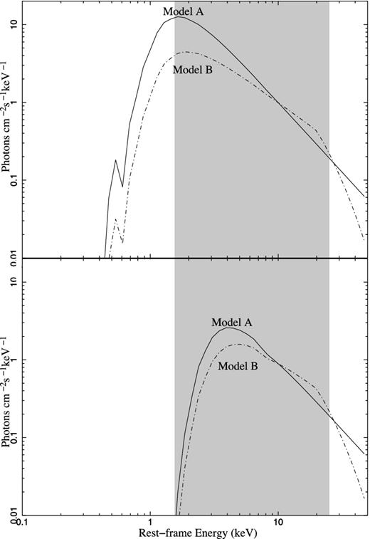
Comparison of the X-ray spectral Models A (solid) and B (dot–dashed) normalized at ∼10 keV. The models are shown for fiducial column densities of 10²² (top) and 10²³ cm⁻² (bottom). The shaded region indicates the effective rest-frame energies sampled by the 0.5–8.0 keV observed spectrum of a source at z ∼ 2.

Application of X-ray spectral models

We now apply our set of spectral models to the X-ray-identified AzTEC SMGs. To correctly fit the intrinsic absorption, which has a strong energy dependence through the photoelectric cross-section, we require accurate source redshift information. This limits us to 32 out of our original sample of 45 X-ray sources (∼63 per cent), including 5 sources in GOODS-N, 14 in GOODS-S and 13 in COSMOS. We favour the spectroscopic redshift, whenever available, over the photometric redshift. Milky Way absorption values of 1.5, 0.9 and 2.5 × 10²⁰ cm⁻² are included for the spectra, depending on whether they were taken in GOODS-N, GOODS-S or COSMOS, respectively. The best-fitting parameters for each set of models, as well as their C-statistic values and associated rest-frame, absorption-corrected 2.0–10.0 keV luminosities, are given in Table 3. As a simple check, we have compared our derived luminosities with those of previously published catalogues (i.e. Alexander et al. 2003; Tozzi et al. 2006) which correlate well with our results.

Table 3.

X-ray spectral fits to identified AzTEC/X-ray sources. Spectral models used are Galactic dust- and intrinsically absorbed AGN power law (PHA(ZPHA(PO)), Model A) and Galactic dust- and intrinsically absorbed power law with an exponential cutoff relating to emission from HMXBs (PHA(ZPHA(HMXB)), Model B). Models that offer the best fit to the X-ray spectra based on our simulations are emphasized in bold. The relevant parameters given here are the intrinsic neutral hydrogen column density (N_H in 10²² cm⁻²), absorption-corrected, rest-frame X-ray luminosity in the 2.0–10.0 keV energy band (L_X in 10⁴³ erg s⁻¹) and X-ray-derived SFR (SFR_X in 1000 M_⊙ yr⁻¹) for Model B assuming the P04 relation. Errors are given at the 90 per cent confidence level.

Chandra ID	Γ_Eff	Model A			Model B
		N_H	L_X	C-stat	N_H	L_X	SFR_X	C-stat
J123616.08+621514.1	0.98\|$ {^{+ 0.23}_{-0.28}} $\|	16.46\|$ {^{+ 7.64}_{-6.20}} $\|	4.40	159.3	6.70\|$ {^{+ 5.76}_{-4.05}} $\|	2.60	26.0	161.0
J123635.86+620707.8	−0.56\|$ {^{+ 0.36}_{-0.45}} $\|	97.94\|$ {^{+ 25.89}_{-29.10}} $\|	8.89	212.7	74.19\|$ {^{+ 25.15}_{-27.01}} $\|	4.51	45.1	213.3
J123711.32+621331.1	0.69\|$ {^{+ 0.52}_{-0.55}} $\|	9.72\|$ {^{+ 21.27}_{-6.95}} $\|	0.92	189.0	< 16.28	0.62	6.2	186.7
J123711.98+621325.8	−0.41\|$ {^{+ 0.65}_{-0.61}} $\|	57.60\|$ {^{+ 45.78}_{-24.30}} $\|	2.70	199.2	38.31\|$ {^{+ 37.00}_{-18.49}} $\|	1.37	13.7	198.8
J123716.63+621733.4	1.17\|$ {^{+ 0.05}_{-0.06}} $\|	2.10\|$ {^{+ 0.25}_{-0.23}} $\|	9.95	236.6	0.52\|$ {^{+ 0.18}_{-0.17}} $\|	8.76	87.6	239.4
J033158.25−274458.8	0.99\|$ {^{+ 0.59}_{-0.55}} $\|	<1.93	0.07	177.3	< 0.83	0.08	0.8	173.8
J033204.48−274643.3	1.39\|$ {^{+ 0.24}_{-0.20}} $\|	1.00\|$ {^{+ 1.02}_{-0.82}} $\|	1.08	187.0	<0.37	1.07	10.7	186.1
J033207.12−275128.6	0.74\|$ {^{+ −0.75}_{-0.75}} $\|	< 14.0	0.04	189.1	<12.3	0.04	0.4	189.2
J033209.71−274249.0	2.22\|$ {^{+ 0.30}_{-0.28}} $\|	< 0.06	0.25	199.4	<0.04	0.34	3.4	238.4
J033212.23−274620.9	0.85\|$ {^{+ 0.15}_{-0.13}} $\|	3.34\|$ {^{+ 0.69}_{-0.68}} $\|	1.00	189.8	1.53\|$ {^{+ 0.58}_{-0.50}} $\|	0.88	8.8	186.6
J033215.32−275037.6	0.96\|$ {^{+ 0.40}_{-0.29}} $\|	0.82\|$ {^{+ 0.41}_{-0.42}} $\|	0.01	204.2	0.34\|$ {^{+ 0.35}_{-0.31}} $\|	0.01	0.1	205.7
J033222.17−274811.6	0.38\|$ {^{+ 0.27}_{-0.28}} $\|	39.19\|$ {^{+ 14.60}_{-10.40}} $\|	3.11	181.8	23.67\|$ {^{+ 10.86}_{-8.72}} $\|	1.66	16.6	182.1
J033222.56−274815.0	−0.43\|$ {^{+ 0.49}_{-0.42}} $\|	94.11\|$ {^{+ 55.73}_{-32.70}} $\|	3.51	182.9	55.83\|$ {^{+ 45.48}_{-21.71}} $\|	1.49	14.9	180.6
J033234.78−275534.0	1.06\|$ {^{+ 0.28}_{-0.31}} $\|	0.43\|$ {^{+ 0.27}_{-0.19}} $\|	4.0e-4	167.9	< 0.45	5.0e−4	5.0e−3	167.7
J033235.18−275215.7	0.64\|$ {^{+ 0.39}_{-0.54}} $\|	5.17\|$ {^{+ 4.38}_{-2.08}} $\|	0.12	179.7	3.17\|$ {^{+ 3.36}_{-1.84}} $\|	0.10	1.0	180.9
J033238.01−274401.2	1.77\|$ {^{+ 1.00}_{-0.88}} $\|	< 5.53	0.14	235.8	<3.95	0.14	1.4	237.6
J033244.02−274635.9	2.01\|$ {^{+ 0.20}_{-0.20}} $\|	< 0.96	3.64	181.6	<0.26	3.15	31.5	230.3
J033246.83−275120.9	0.95\|$ {^{+ 0.52}_{-0.64}} $\|	4.32\|$ {^{+ 4.92}_{-3.16}} $\|	0.20	209.2	< 5.64	0.17	1.7	208.9
J033302.94−275146.9	1.41\|$ {^{+ 0.37}_{-0.26}} $\|	10.36\|$ {^{+ 10.41}_{-6.34}} $\|	14.37	175.5	<7.89	8.69	86.9	182.4
J095905.05+022156.4	0.98\|$ {^{+ 1.40}_{-1.25}} $\|	< 78.54	4.92	47.1	<60.47	2.72	27.2	47.6
J095929.70+021706.4	1.11\|$ {^{+ 1.43}_{-1.23}} $\|	<4.14	0.83	92.7	< 3.28	0.93	9.3	91.8
J095945.15+023021.1	1.24\|$ {^{+ 2.97}_{-1.38}} $\|	<1.01	0.41	140.0	< 0.95	0.57	5.7	139.7
J095953.85+021853.6	0.57\|$ {^{+ 0.58}_{-0.59}} $\|	5.56\|$ {^{+ 3.98}_{-3.14}} $\|	0.79	103.2	3.27\|$ {^{+ 3.66}_{-2.56}} $\|	0.66	6.6	103.7
J095959.96+020633.1	0.52\|$ {^{+ 0.66}_{-0.74}} $\|	5.53\|$ {^{+ 4.30}_{-3.11}} $\|	0.39	79.0	3.71\|$ {^{+ 3.92}_{-2.65}} $\|	0.33	3.3	80.0
J100003.73+020206.4	1.00\|$ {^{+ 2.06}_{-1.53}} $\|	< 124.89	6.16	141.2	<82.08	2.52	25.2	140.8
J100006.11+015239.2	1.77\|$ {^{+ 0.70}_{-0.57}} $\|	< 1.48	2.25	115.6	<0.83	2.26	22.6	118.3
J100006.55+023259.3	1.26\|$ {^{+ 0.58}_{-0.54}} $\|	< 2.98	0.82	87.1	<1.56	0.79	7.9	86.4
J100033.61+014902.0	1.57\|$ {^{+ 0.50}_{-0.45}} $\|	<0.68	0.75	104.8	< 0.29	0.95	9.5	107.5
J100055.34+023441.1	1.85\|$ {^{+ 0.19}_{-0.19}} $\|	< 0.44	24.88	159.2	<0.10	26.84	268.4	181.6
J100107.46+015718.1	1.59\|$ {^{+ 0.79}_{-0.60}} $\|	0.88\|$ {^{+ 2.27}_{-0.86}} $\|	1.46	148.5	< 1.50	1.49	14.9	149.9
J100116.15+023606.9	1.72\|$ {^{+ 0.60}_{-0.56}} $\|	0.20\|$ {^{+ 1.31}_{-0.19}} $\|	5.84	100.3	<0.69	6.72	67.1	102.6
J100139.73+022548.5	3.23\|$ {^{+ 0.79}_{-0.71}} $\|	< 0.05	0.01	81.3	<0.04	0.02	0.2	97.5

Chandra ID	Γ_Eff	Model A			Model B
		N_H	L_X	C-stat	N_H	L_X	SFR_X	C-stat
J123616.08+621514.1	0.98\|$ {^{+ 0.23}_{-0.28}} $\|	16.46\|$ {^{+ 7.64}_{-6.20}} $\|	4.40	159.3	6.70\|$ {^{+ 5.76}_{-4.05}} $\|	2.60	26.0	161.0
J123635.86+620707.8	−0.56\|$ {^{+ 0.36}_{-0.45}} $\|	97.94\|$ {^{+ 25.89}_{-29.10}} $\|	8.89	212.7	74.19\|$ {^{+ 25.15}_{-27.01}} $\|	4.51	45.1	213.3
J123711.32+621331.1	0.69\|$ {^{+ 0.52}_{-0.55}} $\|	9.72\|$ {^{+ 21.27}_{-6.95}} $\|	0.92	189.0	< 16.28	0.62	6.2	186.7
J123711.98+621325.8	−0.41\|$ {^{+ 0.65}_{-0.61}} $\|	57.60\|$ {^{+ 45.78}_{-24.30}} $\|	2.70	199.2	38.31\|$ {^{+ 37.00}_{-18.49}} $\|	1.37	13.7	198.8
J123716.63+621733.4	1.17\|$ {^{+ 0.05}_{-0.06}} $\|	2.10\|$ {^{+ 0.25}_{-0.23}} $\|	9.95	236.6	0.52\|$ {^{+ 0.18}_{-0.17}} $\|	8.76	87.6	239.4
J033158.25−274458.8	0.99\|$ {^{+ 0.59}_{-0.55}} $\|	<1.93	0.07	177.3	< 0.83	0.08	0.8	173.8
J033204.48−274643.3	1.39\|$ {^{+ 0.24}_{-0.20}} $\|	1.00\|$ {^{+ 1.02}_{-0.82}} $\|	1.08	187.0	<0.37	1.07	10.7	186.1
J033207.12−275128.6	0.74\|$ {^{+ −0.75}_{-0.75}} $\|	< 14.0	0.04	189.1	<12.3	0.04	0.4	189.2
J033209.71−274249.0	2.22\|$ {^{+ 0.30}_{-0.28}} $\|	< 0.06	0.25	199.4	<0.04	0.34	3.4	238.4
J033212.23−274620.9	0.85\|$ {^{+ 0.15}_{-0.13}} $\|	3.34\|$ {^{+ 0.69}_{-0.68}} $\|	1.00	189.8	1.53\|$ {^{+ 0.58}_{-0.50}} $\|	0.88	8.8	186.6
J033215.32−275037.6	0.96\|$ {^{+ 0.40}_{-0.29}} $\|	0.82\|$ {^{+ 0.41}_{-0.42}} $\|	0.01	204.2	0.34\|$ {^{+ 0.35}_{-0.31}} $\|	0.01	0.1	205.7
J033222.17−274811.6	0.38\|$ {^{+ 0.27}_{-0.28}} $\|	39.19\|$ {^{+ 14.60}_{-10.40}} $\|	3.11	181.8	23.67\|$ {^{+ 10.86}_{-8.72}} $\|	1.66	16.6	182.1
J033222.56−274815.0	−0.43\|$ {^{+ 0.49}_{-0.42}} $\|	94.11\|$ {^{+ 55.73}_{-32.70}} $\|	3.51	182.9	55.83\|$ {^{+ 45.48}_{-21.71}} $\|	1.49	14.9	180.6
J033234.78−275534.0	1.06\|$ {^{+ 0.28}_{-0.31}} $\|	0.43\|$ {^{+ 0.27}_{-0.19}} $\|	4.0e-4	167.9	< 0.45	5.0e−4	5.0e−3	167.7
J033235.18−275215.7	0.64\|$ {^{+ 0.39}_{-0.54}} $\|	5.17\|$ {^{+ 4.38}_{-2.08}} $\|	0.12	179.7	3.17\|$ {^{+ 3.36}_{-1.84}} $\|	0.10	1.0	180.9
J033238.01−274401.2	1.77\|$ {^{+ 1.00}_{-0.88}} $\|	< 5.53	0.14	235.8	<3.95	0.14	1.4	237.6
J033244.02−274635.9	2.01\|$ {^{+ 0.20}_{-0.20}} $\|	< 0.96	3.64	181.6	<0.26	3.15	31.5	230.3
J033246.83−275120.9	0.95\|$ {^{+ 0.52}_{-0.64}} $\|	4.32\|$ {^{+ 4.92}_{-3.16}} $\|	0.20	209.2	< 5.64	0.17	1.7	208.9
J033302.94−275146.9	1.41\|$ {^{+ 0.37}_{-0.26}} $\|	10.36\|$ {^{+ 10.41}_{-6.34}} $\|	14.37	175.5	<7.89	8.69	86.9	182.4
J095905.05+022156.4	0.98\|$ {^{+ 1.40}_{-1.25}} $\|	< 78.54	4.92	47.1	<60.47	2.72	27.2	47.6
J095929.70+021706.4	1.11\|$ {^{+ 1.43}_{-1.23}} $\|	<4.14	0.83	92.7	< 3.28	0.93	9.3	91.8
J095945.15+023021.1	1.24\|$ {^{+ 2.97}_{-1.38}} $\|	<1.01	0.41	140.0	< 0.95	0.57	5.7	139.7
J095953.85+021853.6	0.57\|$ {^{+ 0.58}_{-0.59}} $\|	5.56\|$ {^{+ 3.98}_{-3.14}} $\|	0.79	103.2	3.27\|$ {^{+ 3.66}_{-2.56}} $\|	0.66	6.6	103.7
J095959.96+020633.1	0.52\|$ {^{+ 0.66}_{-0.74}} $\|	5.53\|$ {^{+ 4.30}_{-3.11}} $\|	0.39	79.0	3.71\|$ {^{+ 3.92}_{-2.65}} $\|	0.33	3.3	80.0
J100003.73+020206.4	1.00\|$ {^{+ 2.06}_{-1.53}} $\|	< 124.89	6.16	141.2	<82.08	2.52	25.2	140.8
J100006.11+015239.2	1.77\|$ {^{+ 0.70}_{-0.57}} $\|	< 1.48	2.25	115.6	<0.83	2.26	22.6	118.3
J100006.55+023259.3	1.26\|$ {^{+ 0.58}_{-0.54}} $\|	< 2.98	0.82	87.1	<1.56	0.79	7.9	86.4
J100033.61+014902.0	1.57\|$ {^{+ 0.50}_{-0.45}} $\|	<0.68	0.75	104.8	< 0.29	0.95	9.5	107.5
J100055.34+023441.1	1.85\|$ {^{+ 0.19}_{-0.19}} $\|	< 0.44	24.88	159.2	<0.10	26.84	268.4	181.6
J100107.46+015718.1	1.59\|$ {^{+ 0.79}_{-0.60}} $\|	0.88\|$ {^{+ 2.27}_{-0.86}} $\|	1.46	148.5	< 1.50	1.49	14.9	149.9
J100116.15+023606.9	1.72\|$ {^{+ 0.60}_{-0.56}} $\|	0.20\|$ {^{+ 1.31}_{-0.19}} $\|	5.84	100.3	<0.69	6.72	67.1	102.6
J100139.73+022548.5	3.23\|$ {^{+ 0.79}_{-0.71}} $\|	< 0.05	0.01	81.3	<0.04	0.02	0.2	97.5

Open in new tab

Table 3.

X-ray spectral fits to identified AzTEC/X-ray sources. Spectral models used are Galactic dust- and intrinsically absorbed AGN power law (PHA(ZPHA(PO)), Model A) and Galactic dust- and intrinsically absorbed power law with an exponential cutoff relating to emission from HMXBs (PHA(ZPHA(HMXB)), Model B). Models that offer the best fit to the X-ray spectra based on our simulations are emphasized in bold. The relevant parameters given here are the intrinsic neutral hydrogen column density (N_H in 10²² cm⁻²), absorption-corrected, rest-frame X-ray luminosity in the 2.0–10.0 keV energy band (L_X in 10⁴³ erg s⁻¹) and X-ray-derived SFR (SFR_X in 1000 M_⊙ yr⁻¹) for Model B assuming the P04 relation. Errors are given at the 90 per cent confidence level.

Chandra ID	Γ_Eff	Model A			Model B
		N_H	L_X	C-stat	N_H	L_X	SFR_X	C-stat
J123616.08+621514.1	0.98\|$ {^{+ 0.23}_{-0.28}} $\|	16.46\|$ {^{+ 7.64}_{-6.20}} $\|	4.40	159.3	6.70\|$ {^{+ 5.76}_{-4.05}} $\|	2.60	26.0	161.0
J123635.86+620707.8	−0.56\|$ {^{+ 0.36}_{-0.45}} $\|	97.94\|$ {^{+ 25.89}_{-29.10}} $\|	8.89	212.7	74.19\|$ {^{+ 25.15}_{-27.01}} $\|	4.51	45.1	213.3
J123711.32+621331.1	0.69\|$ {^{+ 0.52}_{-0.55}} $\|	9.72\|$ {^{+ 21.27}_{-6.95}} $\|	0.92	189.0	< 16.28	0.62	6.2	186.7
J123711.98+621325.8	−0.41\|$ {^{+ 0.65}_{-0.61}} $\|	57.60\|$ {^{+ 45.78}_{-24.30}} $\|	2.70	199.2	38.31\|$ {^{+ 37.00}_{-18.49}} $\|	1.37	13.7	198.8
J123716.63+621733.4	1.17\|$ {^{+ 0.05}_{-0.06}} $\|	2.10\|$ {^{+ 0.25}_{-0.23}} $\|	9.95	236.6	0.52\|$ {^{+ 0.18}_{-0.17}} $\|	8.76	87.6	239.4
J033158.25−274458.8	0.99\|$ {^{+ 0.59}_{-0.55}} $\|	<1.93	0.07	177.3	< 0.83	0.08	0.8	173.8
J033204.48−274643.3	1.39\|$ {^{+ 0.24}_{-0.20}} $\|	1.00\|$ {^{+ 1.02}_{-0.82}} $\|	1.08	187.0	<0.37	1.07	10.7	186.1
J033207.12−275128.6	0.74\|$ {^{+ −0.75}_{-0.75}} $\|	< 14.0	0.04	189.1	<12.3	0.04	0.4	189.2
J033209.71−274249.0	2.22\|$ {^{+ 0.30}_{-0.28}} $\|	< 0.06	0.25	199.4	<0.04	0.34	3.4	238.4
J033212.23−274620.9	0.85\|$ {^{+ 0.15}_{-0.13}} $\|	3.34\|$ {^{+ 0.69}_{-0.68}} $\|	1.00	189.8	1.53\|$ {^{+ 0.58}_{-0.50}} $\|	0.88	8.8	186.6
J033215.32−275037.6	0.96\|$ {^{+ 0.40}_{-0.29}} $\|	0.82\|$ {^{+ 0.41}_{-0.42}} $\|	0.01	204.2	0.34\|$ {^{+ 0.35}_{-0.31}} $\|	0.01	0.1	205.7
J033222.17−274811.6	0.38\|$ {^{+ 0.27}_{-0.28}} $\|	39.19\|$ {^{+ 14.60}_{-10.40}} $\|	3.11	181.8	23.67\|$ {^{+ 10.86}_{-8.72}} $\|	1.66	16.6	182.1
J033222.56−274815.0	−0.43\|$ {^{+ 0.49}_{-0.42}} $\|	94.11\|$ {^{+ 55.73}_{-32.70}} $\|	3.51	182.9	55.83\|$ {^{+ 45.48}_{-21.71}} $\|	1.49	14.9	180.6
J033234.78−275534.0	1.06\|$ {^{+ 0.28}_{-0.31}} $\|	0.43\|$ {^{+ 0.27}_{-0.19}} $\|	4.0e-4	167.9	< 0.45	5.0e−4	5.0e−3	167.7
J033235.18−275215.7	0.64\|$ {^{+ 0.39}_{-0.54}} $\|	5.17\|$ {^{+ 4.38}_{-2.08}} $\|	0.12	179.7	3.17\|$ {^{+ 3.36}_{-1.84}} $\|	0.10	1.0	180.9
J033238.01−274401.2	1.77\|$ {^{+ 1.00}_{-0.88}} $\|	< 5.53	0.14	235.8	<3.95	0.14	1.4	237.6
J033244.02−274635.9	2.01\|$ {^{+ 0.20}_{-0.20}} $\|	< 0.96	3.64	181.6	<0.26	3.15	31.5	230.3
J033246.83−275120.9	0.95\|$ {^{+ 0.52}_{-0.64}} $\|	4.32\|$ {^{+ 4.92}_{-3.16}} $\|	0.20	209.2	< 5.64	0.17	1.7	208.9
J033302.94−275146.9	1.41\|$ {^{+ 0.37}_{-0.26}} $\|	10.36\|$ {^{+ 10.41}_{-6.34}} $\|	14.37	175.5	<7.89	8.69	86.9	182.4
J095905.05+022156.4	0.98\|$ {^{+ 1.40}_{-1.25}} $\|	< 78.54	4.92	47.1	<60.47	2.72	27.2	47.6
J095929.70+021706.4	1.11\|$ {^{+ 1.43}_{-1.23}} $\|	<4.14	0.83	92.7	< 3.28	0.93	9.3	91.8
J095945.15+023021.1	1.24\|$ {^{+ 2.97}_{-1.38}} $\|	<1.01	0.41	140.0	< 0.95	0.57	5.7	139.7
J095953.85+021853.6	0.57\|$ {^{+ 0.58}_{-0.59}} $\|	5.56\|$ {^{+ 3.98}_{-3.14}} $\|	0.79	103.2	3.27\|$ {^{+ 3.66}_{-2.56}} $\|	0.66	6.6	103.7
J095959.96+020633.1	0.52\|$ {^{+ 0.66}_{-0.74}} $\|	5.53\|$ {^{+ 4.30}_{-3.11}} $\|	0.39	79.0	3.71\|$ {^{+ 3.92}_{-2.65}} $\|	0.33	3.3	80.0
J100003.73+020206.4	1.00\|$ {^{+ 2.06}_{-1.53}} $\|	< 124.89	6.16	141.2	<82.08	2.52	25.2	140.8
J100006.11+015239.2	1.77\|$ {^{+ 0.70}_{-0.57}} $\|	< 1.48	2.25	115.6	<0.83	2.26	22.6	118.3
J100006.55+023259.3	1.26\|$ {^{+ 0.58}_{-0.54}} $\|	< 2.98	0.82	87.1	<1.56	0.79	7.9	86.4
J100033.61+014902.0	1.57\|$ {^{+ 0.50}_{-0.45}} $\|	<0.68	0.75	104.8	< 0.29	0.95	9.5	107.5
J100055.34+023441.1	1.85\|$ {^{+ 0.19}_{-0.19}} $\|	< 0.44	24.88	159.2	<0.10	26.84	268.4	181.6
J100107.46+015718.1	1.59\|$ {^{+ 0.79}_{-0.60}} $\|	0.88\|$ {^{+ 2.27}_{-0.86}} $\|	1.46	148.5	< 1.50	1.49	14.9	149.9
J100116.15+023606.9	1.72\|$ {^{+ 0.60}_{-0.56}} $\|	0.20\|$ {^{+ 1.31}_{-0.19}} $\|	5.84	100.3	<0.69	6.72	67.1	102.6
J100139.73+022548.5	3.23\|$ {^{+ 0.79}_{-0.71}} $\|	< 0.05	0.01	81.3	<0.04	0.02	0.2	97.5

Chandra ID	Γ_Eff	Model A			Model B
		N_H	L_X	C-stat	N_H	L_X	SFR_X	C-stat
J123616.08+621514.1	0.98\|$ {^{+ 0.23}_{-0.28}} $\|	16.46\|$ {^{+ 7.64}_{-6.20}} $\|	4.40	159.3	6.70\|$ {^{+ 5.76}_{-4.05}} $\|	2.60	26.0	161.0
J123635.86+620707.8	−0.56\|$ {^{+ 0.36}_{-0.45}} $\|	97.94\|$ {^{+ 25.89}_{-29.10}} $\|	8.89	212.7	74.19\|$ {^{+ 25.15}_{-27.01}} $\|	4.51	45.1	213.3
J123711.32+621331.1	0.69\|$ {^{+ 0.52}_{-0.55}} $\|	9.72\|$ {^{+ 21.27}_{-6.95}} $\|	0.92	189.0	< 16.28	0.62	6.2	186.7
J123711.98+621325.8	−0.41\|$ {^{+ 0.65}_{-0.61}} $\|	57.60\|$ {^{+ 45.78}_{-24.30}} $\|	2.70	199.2	38.31\|$ {^{+ 37.00}_{-18.49}} $\|	1.37	13.7	198.8
J123716.63+621733.4	1.17\|$ {^{+ 0.05}_{-0.06}} $\|	2.10\|$ {^{+ 0.25}_{-0.23}} $\|	9.95	236.6	0.52\|$ {^{+ 0.18}_{-0.17}} $\|	8.76	87.6	239.4
J033158.25−274458.8	0.99\|$ {^{+ 0.59}_{-0.55}} $\|	<1.93	0.07	177.3	< 0.83	0.08	0.8	173.8
J033204.48−274643.3	1.39\|$ {^{+ 0.24}_{-0.20}} $\|	1.00\|$ {^{+ 1.02}_{-0.82}} $\|	1.08	187.0	<0.37	1.07	10.7	186.1
J033207.12−275128.6	0.74\|$ {^{+ −0.75}_{-0.75}} $\|	< 14.0	0.04	189.1	<12.3	0.04	0.4	189.2
J033209.71−274249.0	2.22\|$ {^{+ 0.30}_{-0.28}} $\|	< 0.06	0.25	199.4	<0.04	0.34	3.4	238.4
J033212.23−274620.9	0.85\|$ {^{+ 0.15}_{-0.13}} $\|	3.34\|$ {^{+ 0.69}_{-0.68}} $\|	1.00	189.8	1.53\|$ {^{+ 0.58}_{-0.50}} $\|	0.88	8.8	186.6
J033215.32−275037.6	0.96\|$ {^{+ 0.40}_{-0.29}} $\|	0.82\|$ {^{+ 0.41}_{-0.42}} $\|	0.01	204.2	0.34\|$ {^{+ 0.35}_{-0.31}} $\|	0.01	0.1	205.7
J033222.17−274811.6	0.38\|$ {^{+ 0.27}_{-0.28}} $\|	39.19\|$ {^{+ 14.60}_{-10.40}} $\|	3.11	181.8	23.67\|$ {^{+ 10.86}_{-8.72}} $\|	1.66	16.6	182.1
J033222.56−274815.0	−0.43\|$ {^{+ 0.49}_{-0.42}} $\|	94.11\|$ {^{+ 55.73}_{-32.70}} $\|	3.51	182.9	55.83\|$ {^{+ 45.48}_{-21.71}} $\|	1.49	14.9	180.6
J033234.78−275534.0	1.06\|$ {^{+ 0.28}_{-0.31}} $\|	0.43\|$ {^{+ 0.27}_{-0.19}} $\|	4.0e-4	167.9	< 0.45	5.0e−4	5.0e−3	167.7
J033235.18−275215.7	0.64\|$ {^{+ 0.39}_{-0.54}} $\|	5.17\|$ {^{+ 4.38}_{-2.08}} $\|	0.12	179.7	3.17\|$ {^{+ 3.36}_{-1.84}} $\|	0.10	1.0	180.9
J033238.01−274401.2	1.77\|$ {^{+ 1.00}_{-0.88}} $\|	< 5.53	0.14	235.8	<3.95	0.14	1.4	237.6
J033244.02−274635.9	2.01\|$ {^{+ 0.20}_{-0.20}} $\|	< 0.96	3.64	181.6	<0.26	3.15	31.5	230.3
J033246.83−275120.9	0.95\|$ {^{+ 0.52}_{-0.64}} $\|	4.32\|$ {^{+ 4.92}_{-3.16}} $\|	0.20	209.2	< 5.64	0.17	1.7	208.9
J033302.94−275146.9	1.41\|$ {^{+ 0.37}_{-0.26}} $\|	10.36\|$ {^{+ 10.41}_{-6.34}} $\|	14.37	175.5	<7.89	8.69	86.9	182.4
J095905.05+022156.4	0.98\|$ {^{+ 1.40}_{-1.25}} $\|	< 78.54	4.92	47.1	<60.47	2.72	27.2	47.6
J095929.70+021706.4	1.11\|$ {^{+ 1.43}_{-1.23}} $\|	<4.14	0.83	92.7	< 3.28	0.93	9.3	91.8
J095945.15+023021.1	1.24\|$ {^{+ 2.97}_{-1.38}} $\|	<1.01	0.41	140.0	< 0.95	0.57	5.7	139.7
J095953.85+021853.6	0.57\|$ {^{+ 0.58}_{-0.59}} $\|	5.56\|$ {^{+ 3.98}_{-3.14}} $\|	0.79	103.2	3.27\|$ {^{+ 3.66}_{-2.56}} $\|	0.66	6.6	103.7
J095959.96+020633.1	0.52\|$ {^{+ 0.66}_{-0.74}} $\|	5.53\|$ {^{+ 4.30}_{-3.11}} $\|	0.39	79.0	3.71\|$ {^{+ 3.92}_{-2.65}} $\|	0.33	3.3	80.0
J100003.73+020206.4	1.00\|$ {^{+ 2.06}_{-1.53}} $\|	< 124.89	6.16	141.2	<82.08	2.52	25.2	140.8
J100006.11+015239.2	1.77\|$ {^{+ 0.70}_{-0.57}} $\|	< 1.48	2.25	115.6	<0.83	2.26	22.6	118.3
J100006.55+023259.3	1.26\|$ {^{+ 0.58}_{-0.54}} $\|	< 2.98	0.82	87.1	<1.56	0.79	7.9	86.4
J100033.61+014902.0	1.57\|$ {^{+ 0.50}_{-0.45}} $\|	<0.68	0.75	104.8	< 0.29	0.95	9.5	107.5
J100055.34+023441.1	1.85\|$ {^{+ 0.19}_{-0.19}} $\|	< 0.44	24.88	159.2	<0.10	26.84	268.4	181.6
J100107.46+015718.1	1.59\|$ {^{+ 0.79}_{-0.60}} $\|	0.88\|$ {^{+ 2.27}_{-0.86}} $\|	1.46	148.5	< 1.50	1.49	14.9	149.9
J100116.15+023606.9	1.72\|$ {^{+ 0.60}_{-0.56}} $\|	0.20\|$ {^{+ 1.31}_{-0.19}} $\|	5.84	100.3	<0.69	6.72	67.1	102.6
J100139.73+022548.5	3.23\|$ {^{+ 0.79}_{-0.71}} $\|	< 0.05	0.01	81.3	<0.04	0.02	0.2	97.5

Open in new tab

In order to determine which of our sets of models offer the best fit to the X-ray spectra, we run 2000 Monte Carlo simulations through the GOODNESS command in xspec, which provides the percentage of simulations that have a C-statistic lower than the observed spectrum. The best-fitting spectral models, the ones providing the lowest goodness fraction, have been highlighted in boldface in Table 3. As one might expect, the models with the lowest C-statistics tend to also provide the lowest goodness fractions, indicating a very high probability that the observed spectrum can be characterized by the best-fitting model. Models A and B often show very similar C-statistics, which leads to only a few per cent difference in their goodness fractions. These differences are not statistically significant based on 10 000 FAKEIT simulated fits using an intrinsically absorbed Γ = 1.8 power law as the template spectrum.

We find that ∼53 per cent (17/32) of the AzTEC/X-ray sources have X-ray spectra that immediately favour an AGN origin. Of these, ∼70 per cent show evidence for heavy obscuration with N_H ≳ 10²³ cm⁻². Regardless of the best-fitting spectral model, the majority of AzTEC/X-ray sources (22/32) have 2.0–10.0 keV rest-frame luminosities of ≳10⁴³ erg s⁻¹, heavily favouring an AGN interpretation. Note that the derived luminosities are sensitive to the choice of the X-ray model. For those AzTEC/X-ray sources that favour the SB model Model B, we use the X-ray luminosity to SFR relation of P04 to estimate an SFR, assuming no contribution from a buried AGN. There is some uncertainty in the exact form of the X-ray-to-SFR scaling relation as discussed by Mineo, Gilfanov & Sunyaev (2011); however, many of these relations consider local, low-SFR ( ≲ 10 M_⊙ yr^{− 1}) sources during their construction. As we are concerned with potentially high SFRs, we favour the P04 and Persic & Rephaeli (2007) SFR-X-ray scaling relations; using the Ranalli, Comastri & Setti (2003) relation, or similar, would decrease the estimated SFRs by a factor of ∼2–5. The high X-ray luminosities would require very strong SFRs of the order of ≳10³–10⁴ M_⊙ yr⁻¹, which is pushing the limits for typical SMGs. However, there are five sources with L_X ≲ 10⁴² erg s⁻¹ which are candidates to be SB-powered X-ray sources. These sources account for ∼16 per cent of our X-ray-identified SMG sample, consistent with the SB-powered fraction of LNPS10 (∼17 ± 6 per cent). We caution, however, that this does not necessarily imply that their X-ray emission is dominated by star formation (see Section 3.2.2, Table 4). These results thus show that the bulk of the X-ray emission from our SMG sample is predominately produced by obscured AGNs.

Table 4.

Best-fitting SED parameters for the composite AGN+SB models based on the broad-band photometry of AzTEC/X-ray sources. The predicted X-ray luminosities are compared to those derived from the X-ray spectral modelling (Section 3.1.4) to provide additional weights in calculating the likelihoods. Errors are given at the 1σ confidence level after marginalizing over all other free parameters in the fitted templates. Column 1: Chandra Source ID. Columns 2, 3 and 4: AGN template galaxy outer radius, intrinsic luminosity and visual extinction. Columns 5, 6 and 7: SB template normalization, age and optical depth. Column 8: total model-derived, rest-frame bolometric IR luminosity from the AGN and SB templates over the wavelength range ∼0.001–1500 μm. Column 9: SFR derived from equation (2) (Section 3.2.1) and Columns 5 and 6. Column 10: SED-derived X-ray luminosity. Column 11: fractional contribution of AGN template to total model emission at 1.1 mm. Column 12: fractional contribution of model to observed 1.1 mm flux. Column 13: ln(L) of best-fitting parameters.

	AGN			SB			IR		X-ray
Chandra ID	R	L	A_V	Norm	Age	τ_ν	Lum.	SFR	Lum.	f_{AGN, 1.1 mm}	f_1.1 mm	ln(L)
	(kpc)	(log(L_⊙))	(mag)		(Myr)		(10¹² L_⊙)	(M_⊙ yr⁻¹)	(10⁴³ erg s⁻¹)
(1)	(2)	(3)	(4)	(5)	(6)	(7)	(8)	(9)	(10)	(11)	(12)	(13)
J123616.08+621514.1	0.13\|$ {^{+ 0.15}_{-0.01}} $\|	11.51\|$ {^{+ 0.05}_{-0.18}} $\|	26.10\|$ {^{+ 36.73}_{-17.57}} $\|	8532.40\|$ {^{+ 650.39}_{-490.44}} $\|	44.95\|$ {^{+ 11.53}_{-7.68}} $\|	192.73\|$ {^{+ 7.26}_{-41.29}} $\|	11.10\|$ {^{+ 3.30}_{-3.20}} $\|	901	4.84\|$ {^{+ 0.57}_{-1.26}} $\|	0.00	0.001	−27.94
J123635.86+620707.8	14.30\|$ {^{+ 1.70}_{-14.17}} $\|	10.52\|$ {^{+ 0.11}_{-0.18}} $\|	125.85\|$ {^{+ 2.14}_{-124.84}} $\|	213.66\|$ {^{+ 114.63}_{-92.54}} $\|	56.24\|$ {^{+ 15.75}_{-28.36}} $\|	196.40\|$ {^{+ 3.60}_{-139.53}} $\|	0.23\|$ {^{+ 0.33}_{-0.11}} $\|	12	0.79\|$ {^{+ 0.19}_{-0.21}} $\|	0.91	0.312	−11.40
J123711.32+621331.1	0.91\|$ {^{+ 15.07}_{-0.79}} $\|	10.41\|$ {^{+ 0.11}_{-0.12}} $\|	56.00\|$ {^{+ 31.97}_{-54.99}} $\|	7965.80\|$ {^{+ 182.33}_{-211.12}} $\|	56.66\|$ {^{+ 6.41}_{-10.49}} $\|	198.62\|$ {^{+ 1.37}_{-43.97}} $\|	7.10\|$ {^{+ 2.61}_{-1.21}} $\|	468	0.72\|$ {^{+ 0.13}_{-0.14}} $\|	0.01	0.005	−40.04
J123711.98+621325.8	9.20\|$ {^{+ 6.74}_{-9.08}} $\|	10.81\|$ {^{+ 0.13}_{-0.14}} $\|	74.24\|$ {^{+ 53.54}_{-73.24}} $\|	2685.09\|$ {^{+ 113.89}_{-287.82}} $\|	43.46\|$ {^{+ 12.53}_{-5.76}} $\|	195.49\|$ {^{+ 4.51}_{-42.44}} $\|	3.64\|$ {^{+ 0.65}_{-1.22}} $\|	305	1.39\|$ {^{+ 0.34}_{-0.31}} $\|	0.16	0.059	−9.59
J123716.63+621733.4	15.98\|$ {^{+ 0.02}_{-7.55}} $\|	12.25\|$ {^{+ 0.02}_{-0.01}} $\|	2.10\|$ {^{+ 1.80}_{-1.02}} $\|	9451.94\|$ {^{+ 241.06}_{-179.17}} $\|	1.37\|$ {^{+ 4.85}_{-1.37}} $\|	151.18\|$ {^{+ 46.25}_{-47.75}} $\|	13.00\|$ {^{+ 15.90}_{-0.20}} $\|	8825	17.30\|$ {^{+ 0.63}_{-0.11}} $\|	0.23	0.131	−2868.31
J033158.25−274458.8	14.26\|$ {^{+ 1.74}_{-14.13}} $\|	9.21\|$ {^{+ 0.20}_{-0.13}} $\|	1.00\|$ {^{+ 3.91}_{-0.01}} $\|	1097.69\|$ {^{+ 2.81}_{-4.57}} $\|	70.67\|$ {^{+ 1.33}_{-6.40}} $\|	199.88\|$ {^{+ 0.11}_{-48.26}} $\|	0.67\|$ {^{+ 0.12}_{-0.03}} $\|	32	0.07\|$ {^{+ 0.03}_{-0.01}} $\|	0.05	0.017	−2226.84
J033204.48−274643.3	14.63\|$ {^{+ 1.36}_{-14.49}} $\|	10.67\|$ {^{+ 0.16}_{-0.19}} $\|	1.03\|$ {^{+ 9.78}_{-0.03}} $\|	233.46\|$ {^{+ 96.74}_{-53.53}} $\|	68.27\|$ {^{+ 3.73}_{-10.70}} $\|	105.65\|$ {^{+ 94.31}_{-55.34}} $\|	0.20\|$ {^{+ 0.07}_{-0.06}} $\|	7	1.05\|$ {^{+ 0.35}_{-0.33}} $\|	0.44	0.021	−24.87
J033207.12−275128.6	8.48\|$ {^{+ 7.51}_{-8.35}} $\|	8.97\|$ {^{+ 0.11}_{-0.13}} $\|	67.61\|$ {^{+ 7.31}_{-66.61}} $\|	246.75\|$ {^{+ 13.02}_{-24.16}} $\|	71.54\|$ {^{+ 0.45}_{-13.85}} $\|	197.10\|$ {^{+ 2.88}_{-44.25}} $\|	0.15\|$ {^{+ 0.06}_{-0.01}} $\|	6	0.04\|$ {^{+ 0.01}_{-0.01}} $\|	0.25	0.010	−23.65
J033209.71−274249.0	15.91\|$ {^{+ 0.09}_{-5.84}} $\|	11.00\|$ {^{+ 0.01}_{-0.01}} $\|	1.00\|$ {^{+ 0.01}_{-0.01}} $\|	2040.88\|$ {^{+ 3.22}_{-3.52}} $\|	71.22\|$ {^{+ 0.78}_{-0.50}} $\|	198.51\|$ {^{+ 1.48}_{-31.29}} $\|	1.32\|$ {^{+ 0.02}_{-0.03}} $\|	57	1.87\|$ {^{+ 0.01}_{-0.01}} $\|	0.10	0.070	−135 568.62
J033212.23−274620.9	15.91\|$ {^{+ 0.09}_{-7.64}} $\|	11.25\|$ {^{+ 0.01}_{-0.01}} $\|	1.08\|$ {^{+ 0.89}_{-0.08}} $\|	2106.95\|$ {^{+ 8.74}_{-6.94}} $\|	71.46\|$ {^{+ 0.54}_{-7.25}} $\|	193.54\|$ {^{+ 6.45}_{-42.36}} $\|	1.43\|$ {^{+ 0.26}_{-0.02}} $\|	59	2.94\|$ {^{+ 0.02}_{-0.01}} $\|	0.11	0.038	−3350.01
J033215.32−275037.6	5.65\|$ {^{+ 10.34}_{-5.53}} $\|	10.70\|$ {^{+ 0.05}_{-0.29}} $\|	1.03\|$ {^{+ 1.99}_{-0.03}} $\|	3280.00\|$ {^{+ 23.15}_{-27.60}} $\|	70.60\|$ {^{+ 1.40}_{-6.14}} $\|	50.31\|$ {^{+ 47.39}_{-0.30}} $\|	2.04\|$ {^{+ 0.34}_{-0.10}} $\|	96	1.10\|$ {^{+ 0.09}_{-0.44}} $\|	0.01	0.004	−1280.28
J033222.17−274811.6	15.38\|$ {^{+ 0.62}_{-15.11}} $\|	11.27\|$ {^{+ 0.07}_{-0.02}} $\|	4.46\|$ {^{+ 10.92}_{-2.38}} $\|	2483.75\|$ {^{+ 80.91}_{-22.82}} $\|	44.38\|$ {^{+ 11.97}_{-6.94}} $\|	53.72\|$ {^{+ 43.88}_{-3.72}} $\|	3.39\|$ {^{+ 0.78}_{-0.97}} $\|	269	3.08\|$ {^{+ 0.46}_{-0.13}} $\|	0.18	0.098	−60.08
J033222.56−274815.0	13.81\|$ {^{+ 2.19}_{-13.68}} $\|	10.85\|$ {^{+ 0.19}_{-0.08}} $\|	1.08\|$ {^{+ 2.24}_{-0.08}} $\|	3844.91\|$ {^{+ 37.39}_{-72.25}} $\|	71.97\|$ {^{+ 0.03}_{-7.59}} $\|	57.91\|$ {^{+ 40.71}_{-7.88}} $\|	2.32\|$ {^{+ 0.51}_{-0.01}} $\|	105	1.48\|$ {^{+ 0.56}_{-0.22}} $\|	0.04	0.022	−62.72
J033235.18−275215.7	0.15\|$ {^{+ 0.10}_{-0.02}} $\|	9.76\|$ {^{+ 0.02}_{-0.01}} $\|	50.82\|$ {^{+ 1.18}_{-18.32}} $\|	109.77\|$ {^{+ 5.04}_{-6.44}} $\|	71.98\|$ {^{+ 0.02}_{-7.41}} $\|	198.63\|$ {^{+ 1.37}_{-46.96}} $\|	0.07\|$ {^{+ 0.02}_{-0.01}} $\|	3	0.18\|$ {^{+ 0.01}_{-0.01}} $\|	0.02	0.000	−302.13
J033238.01−274401.2	15.69\|$ {^{+ 0.31}_{-15.56}} $\|	9.51\|$ {^{+ 0.07}_{-0.15}} $\|	10.90\|$ {^{+ 19.09}_{-9.90}} $\|	1019.35\|$ {^{+ 22.35}_{-21.65}} $\|	36.06\|$ {^{+ 8.06}_{-8.69}} $\|	198.61\|$ {^{+ 1.39}_{-43.73}} $\|	1.70\|$ {^{+ 0.50}_{-0.38}} $\|	167	0.13\|$ {^{+ 0.02}_{-0.03}} $\|	0.10	0.024	−111.65
J033244.02−274635.9	0.13\|$ {^{+ 0.11}_{-0.01}} $\|	11.51\|$ {^{+ 0.04}_{-0.01}} $\|	5.92\|$ {^{+ 0.08}_{-1.70}} $\|	2523.09\|$ {^{+ 38.84}_{-38.49}} $\|	57.21\|$ {^{+ 6.09}_{-11.43}} $\|	101.31\|$ {^{+ 45.07}_{-46.64}} $\|	2.53\|$ {^{+ 0.92}_{-0.35}} $\|	144	4.75\|$ {^{+ 0.44}_{-0.16}} $\|	0.00	0.000	−89.91
J033246.83−275120.9	0.14\|$ {^{+ 0.11}_{-0.01}} $\|	10.00\|$ {^{+ 0.02}_{-0.01}} $\|	30.97\|$ {^{+ 0.03}_{-14.38}} $\|	868.22\|$ {^{+ 9.67}_{-7.11}} $\|	71.34\|$ {^{+ 0.66}_{-6.77}} $\|	197.29\|$ {^{+ 2.71}_{-45.44}} $\|	0.53\|$ {^{+ 0.10}_{-0.01}} $\|	24	0.30\|$ {^{+ 0.01}_{-0.01}} $\|	0.00	0.000	−4001.74
J033302.94−275146.9	0.25\|$ {^{+ 0.22}_{-0.01}} $\|	12.26\|$ {^{+ 0.03}_{-0.01}} $\|	6.96\|$ {^{+ 8.01}_{-2.80}} $\|	7001.07\|$ {^{+ 139.78}_{-215.29}} $\|	44.91\|$ {^{+ 11.39}_{-7.35}} $\|	100.74\|$ {^{+ 45.91}_{-46.93}} $\|	10.70\|$ {^{+ 2.30}_{-2.60}} $\|	741	17.39\|$ {^{+ 1.32}_{-0.25}} $\|	0.00	0.001	−61.65
J095905.05+022156.4	2.39\|$ {^{+ 13.57}_{-2.26}} $\|	11.40\|$ {^{+ 0.13}_{-0.13}} $\|	7.42\|$ {^{+ 120.08}_{-6.42}} $\|	8693.26\|$ {^{+ 308.01}_{-550.64}} $\|	44.42\|$ {^{+ 11.06}_{-6.48}} $\|	151.03\|$ {^{+ 44.55}_{-47.51}} $\|	11.40\|$ {^{+ 2.60}_{-3.30}} $\|	942	4.08\|$ {^{+ 0.93}_{-0.88}} $\|	0.01	0.009	−4.53
J095929.70+021706.4	6.22\|$ {^{+ 9.78}_{-6.09}} $\|	10.61\|$ {^{+ 0.12}_{-0.13}} $\|	16.33\|$ {^{+ 1.22}_{-15.32}} $\|	4819.83\|$ {^{+ 39.78}_{-238.62}} $\|	71.79\|$ {^{+ 0.21}_{-12.12}} $\|	148.38\|$ {^{+ 48.37}_{-44.31}} $\|	2.87\|$ {^{+ 0.94}_{-0.06}} $\|	133	0.97\|$ {^{+ 0.21}_{-0.22}} $\|	0.06	0.027	−2.33
J095945.15+023021.1	9.82\|$ {^{+ 6.00}_{-8.78}} $\|	10.75\|$ {^{+ 0.01}_{-0.01}} $\|	1.31\|$ {^{+ 0.68}_{-0.31}} $\|	1797.01\|$ {^{+ 8.54}_{-19.38}} $\|	71.87\|$ {^{+ 0.13}_{-7.66}} $\|	60.11\|$ {^{+ 38.85}_{-10.11}} $\|	1.11\|$ {^{+ 0.23}_{-0.01}} $\|	49	1.19\|$ {^{+ 0.04}_{-0.01}} $\|	0.04	0.007	−588.57
J095953.85+021853.6	0.13\|$ {^{+ 0.11}_{-0.01}} $\|	10.52\|$ {^{+ 0.08}_{-0.01}} $\|	31.08\|$ {^{+ 5.99}_{-14.31}} $\|	1677.68\|$ {^{+ 15.21}_{-14.04}} $\|	71.88\|$ {^{+ 0.12}_{-7.63}} $\|	195.74\|$ {^{+ 4.25}_{-44.40}} $\|	1.02\|$ {^{+ 0.22}_{-0.01}} $\|	46	0.78\|$ {^{+ 0.15}_{-0.03}} $\|	0.00	0.000	−222.44
J095959.96+020633.1	12.49\|$ {^{+ 3.50}_{-12.37}} $\|	10.09\|$ {^{+ 0.07}_{-0.02}} $\|	52.38\|$ {^{+ 0.20}_{-33.85}} $\|	669.15\|$ {^{+ 7.07}_{-11.74}} $\|	46.63\|$ {^{+ 8.96}_{-9.36}} $\|	190.37\|$ {^{+ 9.63}_{-39.41}} $\|	0.82\|$ {^{+ 0.27}_{-0.19}} $\|	65	0.36\|$ {^{+ 0.05}_{-0.02}} $\|	0.51	0.085	−174.35
J100003.73+020206.4	12.25\|$ {^{+ 3.75}_{-12.12}} $\|	11.18\|$ {^{+ 0.11}_{-0.17}} $\|	121.10\|$ {^{+ 6.90}_{-120.08}} $\|	995.74\|$ {^{+ 44.76}_{-169.08}} $\|	70.55\|$ {^{+ 1.45}_{-24.73}} $\|	54.92\|$ {^{+ 43.17}_{-4.92}} $\|	0.76\|$ {^{+ 0.56}_{-0.11}} $\|	29	2.65\|$ {^{+ 0.58}_{-0.74}} $\|	0.75	0.212	−18.55
J100006.11+015239.2	12.59\|$ {^{+ 3.41}_{-12.47}} $\|	11.07\|$ {^{+ 0.13}_{-0.16}} $\|	7.90\|$ {^{+ 0.02}_{-6.89}} $\|	2859.00\|$ {^{+ 34.58}_{-188.34}} $\|	71.82\|$ {^{+ 0.18}_{-13.53}} $\|	185.32\|$ {^{+ 14.67}_{-33.72}} $\|	1.80\|$ {^{+ 0.64}_{-0.09}} $\|	78	2.21\|$ {^{+ 0.57}_{-0.56}} $\|	0.21	0.063	−11.98
J100006.55+023259.3	0.92\|$ {^{+ 2.81}_{-0.75}} $\|	10.43\|$ {^{+ 0.07}_{-0.11}} $\|	1.01\|$ {^{+ 0.93}_{-0.01}} $\|	1905.42\|$ {^{+ 19.50}_{-16.07}} $\|	71.04\|$ {^{+ 0.96}_{-6.52}} $\|	194.34\|$ {^{+ 5.66}_{-42.19}} $\|	1.17\|$ {^{+ 0.21}_{-0.04}} $\|	54	0.68\|$ {^{+ 0.07}_{-0.13}} $\|	0.00	0.000	−4319.74
J100033.61+014902.0	6.84\|$ {^{+ 9.16}_{-5.87}} $\|	10.64\|$ {^{+ 0.13}_{-0.12}} $\|	1.47\|$ {^{+ 0.09}_{-0.34}} $\|	2418.84\|$ {^{+ 26.17}_{-41.92}} $\|	71.81\|$ {^{+ 0.19}_{-7.48}} $\|	193.21\|$ {^{+ 6.79}_{-41.24}} $\|	1.47\|$ {^{+ 0.31}_{-0.03}} $\|	66	1.00\|$ {^{+ 0.23}_{-0.21}} $\|	0.03	0.005	−323.60
J100055.34+023441.1	15.73\|$ {^{+ 0.26}_{-7.54}} $\|	12.75\|$ {^{+ 0.02}_{-0.01}} $\|	2.32\|$ {^{+ 0.03}_{-0.31}} $\|	1366.06\|$ {^{+ 69.89}_{-49.88}} $\|	17.24\|$ {^{+ 8.42}_{-6.91}} $\|	54.57\|$ {^{+ 43.64}_{-4.57}} $\|	9.53\|$ {^{+ 0.69}_{-0.73}} $\|	576	40.84\|$ {^{+ 1.98}_{-0.37}} $\|	0.47	0.076	−18 184.24
J100107.46+015718.1	15.60\|$ {^{+ 0.40}_{-12.86}} $\|	10.87\|$ {^{+ 0.25}_{-0.08}} $\|	2.43\|$ {^{+ 5.60}_{-1.42}} $\|	2202.64\|$ {^{+ 101.75}_{-130.42}} $\|	70.94\|$ {^{+ 1.06}_{-6.85}} $\|	197.34\|$ {^{+ 2.66}_{-46.46}} $\|	1.40\|$ {^{+ 0.31}_{-0.06}} $\|	63	1.52\|$ {^{+ 0.86}_{-0.23}} $\|	0.12	0.028	−93.88
J100116.15+023606.9	0.13\|$ {^{+ 0.11}_{-0.01}} $\|	11.82\|$ {^{+ 0.11}_{-0.15}} $\|	8.08\|$ {^{+ 0.01}_{-0.07}} $\|	4426.14\|$ {^{+ 18.13}_{-15.78}} $\|	64.22\|$ {^{+ 7.29}_{-6.83}} $\|	196.37\|$ {^{+ 3.62}_{-43.90}} $\|	3.85\|$ {^{+ 0.71}_{-0.63}} $\|	178	8.23\|$ {^{+ 1.68}_{-1.96}} $\|	0.00	0.000	−1096.50
J100139.73+022548.5	0.99\|$ {^{+ 0.32}_{-0.48}} $\|	9.00\|$ {^{+ 0.01}_{-0.01}} $\|	1.00\|$ {^{+ 0.01}_{-0.01}} $\|	10.41\|$ {^{+ 0.08}_{-0.09}} $\|	2.07\|$ {^{+ 4.26}_{-2.07}} $\|	51.98\|$ {^{+ 44.46}_{-1.96}} $\|	0.01\|$ {^{+ 0.02}_{-0.01}} $\|	9	0.04\|$ {^{+ 0.01}_{-0.01}} $\|	0.32	0.001	−187 114.26

	AGN			SB			IR		X-ray
Chandra ID	R	L	A_V	Norm	Age	τ_ν	Lum.	SFR	Lum.	f_{AGN, 1.1 mm}	f_1.1 mm	ln(L)
	(kpc)	(log(L_⊙))	(mag)		(Myr)		(10¹² L_⊙)	(M_⊙ yr⁻¹)	(10⁴³ erg s⁻¹)
(1)	(2)	(3)	(4)	(5)	(6)	(7)	(8)	(9)	(10)	(11)	(12)	(13)
J123616.08+621514.1	0.13\|$ {^{+ 0.15}_{-0.01}} $\|	11.51\|$ {^{+ 0.05}_{-0.18}} $\|	26.10\|$ {^{+ 36.73}_{-17.57}} $\|	8532.40\|$ {^{+ 650.39}_{-490.44}} $\|	44.95\|$ {^{+ 11.53}_{-7.68}} $\|	192.73\|$ {^{+ 7.26}_{-41.29}} $\|	11.10\|$ {^{+ 3.30}_{-3.20}} $\|	901	4.84\|$ {^{+ 0.57}_{-1.26}} $\|	0.00	0.001	−27.94
J123635.86+620707.8	14.30\|$ {^{+ 1.70}_{-14.17}} $\|	10.52\|$ {^{+ 0.11}_{-0.18}} $\|	125.85\|$ {^{+ 2.14}_{-124.84}} $\|	213.66\|$ {^{+ 114.63}_{-92.54}} $\|	56.24\|$ {^{+ 15.75}_{-28.36}} $\|	196.40\|$ {^{+ 3.60}_{-139.53}} $\|	0.23\|$ {^{+ 0.33}_{-0.11}} $\|	12	0.79\|$ {^{+ 0.19}_{-0.21}} $\|	0.91	0.312	−11.40
J123711.32+621331.1	0.91\|$ {^{+ 15.07}_{-0.79}} $\|	10.41\|$ {^{+ 0.11}_{-0.12}} $\|	56.00\|$ {^{+ 31.97}_{-54.99}} $\|	7965.80\|$ {^{+ 182.33}_{-211.12}} $\|	56.66\|$ {^{+ 6.41}_{-10.49}} $\|	198.62\|$ {^{+ 1.37}_{-43.97}} $\|	7.10\|$ {^{+ 2.61}_{-1.21}} $\|	468	0.72\|$ {^{+ 0.13}_{-0.14}} $\|	0.01	0.005	−40.04
J123711.98+621325.8	9.20\|$ {^{+ 6.74}_{-9.08}} $\|	10.81\|$ {^{+ 0.13}_{-0.14}} $\|	74.24\|$ {^{+ 53.54}_{-73.24}} $\|	2685.09\|$ {^{+ 113.89}_{-287.82}} $\|	43.46\|$ {^{+ 12.53}_{-5.76}} $\|	195.49\|$ {^{+ 4.51}_{-42.44}} $\|	3.64\|$ {^{+ 0.65}_{-1.22}} $\|	305	1.39\|$ {^{+ 0.34}_{-0.31}} $\|	0.16	0.059	−9.59
J123716.63+621733.4	15.98\|$ {^{+ 0.02}_{-7.55}} $\|	12.25\|$ {^{+ 0.02}_{-0.01}} $\|	2.10\|$ {^{+ 1.80}_{-1.02}} $\|	9451.94\|$ {^{+ 241.06}_{-179.17}} $\|	1.37\|$ {^{+ 4.85}_{-1.37}} $\|	151.18\|$ {^{+ 46.25}_{-47.75}} $\|	13.00\|$ {^{+ 15.90}_{-0.20}} $\|	8825	17.30\|$ {^{+ 0.63}_{-0.11}} $\|	0.23	0.131	−2868.31
J033158.25−274458.8	14.26\|$ {^{+ 1.74}_{-14.13}} $\|	9.21\|$ {^{+ 0.20}_{-0.13}} $\|	1.00\|$ {^{+ 3.91}_{-0.01}} $\|	1097.69\|$ {^{+ 2.81}_{-4.57}} $\|	70.67\|$ {^{+ 1.33}_{-6.40}} $\|	199.88\|$ {^{+ 0.11}_{-48.26}} $\|	0.67\|$ {^{+ 0.12}_{-0.03}} $\|	32	0.07\|$ {^{+ 0.03}_{-0.01}} $\|	0.05	0.017	−2226.84
J033204.48−274643.3	14.63\|$ {^{+ 1.36}_{-14.49}} $\|	10.67\|$ {^{+ 0.16}_{-0.19}} $\|	1.03\|$ {^{+ 9.78}_{-0.03}} $\|	233.46\|$ {^{+ 96.74}_{-53.53}} $\|	68.27\|$ {^{+ 3.73}_{-10.70}} $\|	105.65\|$ {^{+ 94.31}_{-55.34}} $\|	0.20\|$ {^{+ 0.07}_{-0.06}} $\|	7	1.05\|$ {^{+ 0.35}_{-0.33}} $\|	0.44	0.021	−24.87
J033207.12−275128.6	8.48\|$ {^{+ 7.51}_{-8.35}} $\|	8.97\|$ {^{+ 0.11}_{-0.13}} $\|	67.61\|$ {^{+ 7.31}_{-66.61}} $\|	246.75\|$ {^{+ 13.02}_{-24.16}} $\|	71.54\|$ {^{+ 0.45}_{-13.85}} $\|	197.10\|$ {^{+ 2.88}_{-44.25}} $\|	0.15\|$ {^{+ 0.06}_{-0.01}} $\|	6	0.04\|$ {^{+ 0.01}_{-0.01}} $\|	0.25	0.010	−23.65
J033209.71−274249.0	15.91\|$ {^{+ 0.09}_{-5.84}} $\|	11.00\|$ {^{+ 0.01}_{-0.01}} $\|	1.00\|$ {^{+ 0.01}_{-0.01}} $\|	2040.88\|$ {^{+ 3.22}_{-3.52}} $\|	71.22\|$ {^{+ 0.78}_{-0.50}} $\|	198.51\|$ {^{+ 1.48}_{-31.29}} $\|	1.32\|$ {^{+ 0.02}_{-0.03}} $\|	57	1.87\|$ {^{+ 0.01}_{-0.01}} $\|	0.10	0.070	−135 568.62
J033212.23−274620.9	15.91\|$ {^{+ 0.09}_{-7.64}} $\|	11.25\|$ {^{+ 0.01}_{-0.01}} $\|	1.08\|$ {^{+ 0.89}_{-0.08}} $\|	2106.95\|$ {^{+ 8.74}_{-6.94}} $\|	71.46\|$ {^{+ 0.54}_{-7.25}} $\|	193.54\|$ {^{+ 6.45}_{-42.36}} $\|	1.43\|$ {^{+ 0.26}_{-0.02}} $\|	59	2.94\|$ {^{+ 0.02}_{-0.01}} $\|	0.11	0.038	−3350.01
J033215.32−275037.6	5.65\|$ {^{+ 10.34}_{-5.53}} $\|	10.70\|$ {^{+ 0.05}_{-0.29}} $\|	1.03\|$ {^{+ 1.99}_{-0.03}} $\|	3280.00\|$ {^{+ 23.15}_{-27.60}} $\|	70.60\|$ {^{+ 1.40}_{-6.14}} $\|	50.31\|$ {^{+ 47.39}_{-0.30}} $\|	2.04\|$ {^{+ 0.34}_{-0.10}} $\|	96	1.10\|$ {^{+ 0.09}_{-0.44}} $\|	0.01	0.004	−1280.28
J033222.17−274811.6	15.38\|$ {^{+ 0.62}_{-15.11}} $\|	11.27\|$ {^{+ 0.07}_{-0.02}} $\|	4.46\|$ {^{+ 10.92}_{-2.38}} $\|	2483.75\|$ {^{+ 80.91}_{-22.82}} $\|	44.38\|$ {^{+ 11.97}_{-6.94}} $\|	53.72\|$ {^{+ 43.88}_{-3.72}} $\|	3.39\|$ {^{+ 0.78}_{-0.97}} $\|	269	3.08\|$ {^{+ 0.46}_{-0.13}} $\|	0.18	0.098	−60.08
J033222.56−274815.0	13.81\|$ {^{+ 2.19}_{-13.68}} $\|	10.85\|$ {^{+ 0.19}_{-0.08}} $\|	1.08\|$ {^{+ 2.24}_{-0.08}} $\|	3844.91\|$ {^{+ 37.39}_{-72.25}} $\|	71.97\|$ {^{+ 0.03}_{-7.59}} $\|	57.91\|$ {^{+ 40.71}_{-7.88}} $\|	2.32\|$ {^{+ 0.51}_{-0.01}} $\|	105	1.48\|$ {^{+ 0.56}_{-0.22}} $\|	0.04	0.022	−62.72
J033235.18−275215.7	0.15\|$ {^{+ 0.10}_{-0.02}} $\|	9.76\|$ {^{+ 0.02}_{-0.01}} $\|	50.82\|$ {^{+ 1.18}_{-18.32}} $\|	109.77\|$ {^{+ 5.04}_{-6.44}} $\|	71.98\|$ {^{+ 0.02}_{-7.41}} $\|	198.63\|$ {^{+ 1.37}_{-46.96}} $\|	0.07\|$ {^{+ 0.02}_{-0.01}} $\|	3	0.18\|$ {^{+ 0.01}_{-0.01}} $\|	0.02	0.000	−302.13
J033238.01−274401.2	15.69\|$ {^{+ 0.31}_{-15.56}} $\|	9.51\|$ {^{+ 0.07}_{-0.15}} $\|	10.90\|$ {^{+ 19.09}_{-9.90}} $\|	1019.35\|$ {^{+ 22.35}_{-21.65}} $\|	36.06\|$ {^{+ 8.06}_{-8.69}} $\|	198.61\|$ {^{+ 1.39}_{-43.73}} $\|	1.70\|$ {^{+ 0.50}_{-0.38}} $\|	167	0.13\|$ {^{+ 0.02}_{-0.03}} $\|	0.10	0.024	−111.65
J033244.02−274635.9	0.13\|$ {^{+ 0.11}_{-0.01}} $\|	11.51\|$ {^{+ 0.04}_{-0.01}} $\|	5.92\|$ {^{+ 0.08}_{-1.70}} $\|	2523.09\|$ {^{+ 38.84}_{-38.49}} $\|	57.21\|$ {^{+ 6.09}_{-11.43}} $\|	101.31\|$ {^{+ 45.07}_{-46.64}} $\|	2.53\|$ {^{+ 0.92}_{-0.35}} $\|	144	4.75\|$ {^{+ 0.44}_{-0.16}} $\|	0.00	0.000	−89.91
J033246.83−275120.9	0.14\|$ {^{+ 0.11}_{-0.01}} $\|	10.00\|$ {^{+ 0.02}_{-0.01}} $\|	30.97\|$ {^{+ 0.03}_{-14.38}} $\|	868.22\|$ {^{+ 9.67}_{-7.11}} $\|	71.34\|$ {^{+ 0.66}_{-6.77}} $\|	197.29\|$ {^{+ 2.71}_{-45.44}} $\|	0.53\|$ {^{+ 0.10}_{-0.01}} $\|	24	0.30\|$ {^{+ 0.01}_{-0.01}} $\|	0.00	0.000	−4001.74
J033302.94−275146.9	0.25\|$ {^{+ 0.22}_{-0.01}} $\|	12.26\|$ {^{+ 0.03}_{-0.01}} $\|	6.96\|$ {^{+ 8.01}_{-2.80}} $\|	7001.07\|$ {^{+ 139.78}_{-215.29}} $\|	44.91\|$ {^{+ 11.39}_{-7.35}} $\|	100.74\|$ {^{+ 45.91}_{-46.93}} $\|	10.70\|$ {^{+ 2.30}_{-2.60}} $\|	741	17.39\|$ {^{+ 1.32}_{-0.25}} $\|	0.00	0.001	−61.65
J095905.05+022156.4	2.39\|$ {^{+ 13.57}_{-2.26}} $\|	11.40\|$ {^{+ 0.13}_{-0.13}} $\|	7.42\|$ {^{+ 120.08}_{-6.42}} $\|	8693.26\|$ {^{+ 308.01}_{-550.64}} $\|	44.42\|$ {^{+ 11.06}_{-6.48}} $\|	151.03\|$ {^{+ 44.55}_{-47.51}} $\|	11.40\|$ {^{+ 2.60}_{-3.30}} $\|	942	4.08\|$ {^{+ 0.93}_{-0.88}} $\|	0.01	0.009	−4.53
J095929.70+021706.4	6.22\|$ {^{+ 9.78}_{-6.09}} $\|	10.61\|$ {^{+ 0.12}_{-0.13}} $\|	16.33\|$ {^{+ 1.22}_{-15.32}} $\|	4819.83\|$ {^{+ 39.78}_{-238.62}} $\|	71.79\|$ {^{+ 0.21}_{-12.12}} $\|	148.38\|$ {^{+ 48.37}_{-44.31}} $\|	2.87\|$ {^{+ 0.94}_{-0.06}} $\|	133	0.97\|$ {^{+ 0.21}_{-0.22}} $\|	0.06	0.027	−2.33
J095945.15+023021.1	9.82\|$ {^{+ 6.00}_{-8.78}} $\|	10.75\|$ {^{+ 0.01}_{-0.01}} $\|	1.31\|$ {^{+ 0.68}_{-0.31}} $\|	1797.01\|$ {^{+ 8.54}_{-19.38}} $\|	71.87\|$ {^{+ 0.13}_{-7.66}} $\|	60.11\|$ {^{+ 38.85}_{-10.11}} $\|	1.11\|$ {^{+ 0.23}_{-0.01}} $\|	49	1.19\|$ {^{+ 0.04}_{-0.01}} $\|	0.04	0.007	−588.57
J095953.85+021853.6	0.13\|$ {^{+ 0.11}_{-0.01}} $\|	10.52\|$ {^{+ 0.08}_{-0.01}} $\|	31.08\|$ {^{+ 5.99}_{-14.31}} $\|	1677.68\|$ {^{+ 15.21}_{-14.04}} $\|	71.88\|$ {^{+ 0.12}_{-7.63}} $\|	195.74\|$ {^{+ 4.25}_{-44.40}} $\|	1.02\|$ {^{+ 0.22}_{-0.01}} $\|	46	0.78\|$ {^{+ 0.15}_{-0.03}} $\|	0.00	0.000	−222.44
J095959.96+020633.1	12.49\|$ {^{+ 3.50}_{-12.37}} $\|	10.09\|$ {^{+ 0.07}_{-0.02}} $\|	52.38\|$ {^{+ 0.20}_{-33.85}} $\|	669.15\|$ {^{+ 7.07}_{-11.74}} $\|	46.63\|$ {^{+ 8.96}_{-9.36}} $\|	190.37\|$ {^{+ 9.63}_{-39.41}} $\|	0.82\|$ {^{+ 0.27}_{-0.19}} $\|	65	0.36\|$ {^{+ 0.05}_{-0.02}} $\|	0.51	0.085	−174.35
J100003.73+020206.4	12.25\|$ {^{+ 3.75}_{-12.12}} $\|	11.18\|$ {^{+ 0.11}_{-0.17}} $\|	121.10\|$ {^{+ 6.90}_{-120.08}} $\|	995.74\|$ {^{+ 44.76}_{-169.08}} $\|	70.55\|$ {^{+ 1.45}_{-24.73}} $\|	54.92\|$ {^{+ 43.17}_{-4.92}} $\|	0.76\|$ {^{+ 0.56}_{-0.11}} $\|	29	2.65\|$ {^{+ 0.58}_{-0.74}} $\|	0.75	0.212	−18.55
J100006.11+015239.2	12.59\|$ {^{+ 3.41}_{-12.47}} $\|	11.07\|$ {^{+ 0.13}_{-0.16}} $\|	7.90\|$ {^{+ 0.02}_{-6.89}} $\|	2859.00\|$ {^{+ 34.58}_{-188.34}} $\|	71.82\|$ {^{+ 0.18}_{-13.53}} $\|	185.32\|$ {^{+ 14.67}_{-33.72}} $\|	1.80\|$ {^{+ 0.64}_{-0.09}} $\|	78	2.21\|$ {^{+ 0.57}_{-0.56}} $\|	0.21	0.063	−11.98
J100006.55+023259.3	0.92\|$ {^{+ 2.81}_{-0.75}} $\|	10.43\|$ {^{+ 0.07}_{-0.11}} $\|	1.01\|$ {^{+ 0.93}_{-0.01}} $\|	1905.42\|$ {^{+ 19.50}_{-16.07}} $\|	71.04\|$ {^{+ 0.96}_{-6.52}} $\|	194.34\|$ {^{+ 5.66}_{-42.19}} $\|	1.17\|$ {^{+ 0.21}_{-0.04}} $\|	54	0.68\|$ {^{+ 0.07}_{-0.13}} $\|	0.00	0.000	−4319.74
J100033.61+014902.0	6.84\|$ {^{+ 9.16}_{-5.87}} $\|	10.64\|$ {^{+ 0.13}_{-0.12}} $\|	1.47\|$ {^{+ 0.09}_{-0.34}} $\|	2418.84\|$ {^{+ 26.17}_{-41.92}} $\|	71.81\|$ {^{+ 0.19}_{-7.48}} $\|	193.21\|$ {^{+ 6.79}_{-41.24}} $\|	1.47\|$ {^{+ 0.31}_{-0.03}} $\|	66	1.00\|$ {^{+ 0.23}_{-0.21}} $\|	0.03	0.005	−323.60
J100055.34+023441.1	15.73\|$ {^{+ 0.26}_{-7.54}} $\|	12.75\|$ {^{+ 0.02}_{-0.01}} $\|	2.32\|$ {^{+ 0.03}_{-0.31}} $\|	1366.06\|$ {^{+ 69.89}_{-49.88}} $\|	17.24\|$ {^{+ 8.42}_{-6.91}} $\|	54.57\|$ {^{+ 43.64}_{-4.57}} $\|	9.53\|$ {^{+ 0.69}_{-0.73}} $\|	576	40.84\|$ {^{+ 1.98}_{-0.37}} $\|	0.47	0.076	−18 184.24
J100107.46+015718.1	15.60\|$ {^{+ 0.40}_{-12.86}} $\|	10.87\|$ {^{+ 0.25}_{-0.08}} $\|	2.43\|$ {^{+ 5.60}_{-1.42}} $\|	2202.64\|$ {^{+ 101.75}_{-130.42}} $\|	70.94\|$ {^{+ 1.06}_{-6.85}} $\|	197.34\|$ {^{+ 2.66}_{-46.46}} $\|	1.40\|$ {^{+ 0.31}_{-0.06}} $\|	63	1.52\|$ {^{+ 0.86}_{-0.23}} $\|	0.12	0.028	−93.88
J100116.15+023606.9	0.13\|$ {^{+ 0.11}_{-0.01}} $\|	11.82\|$ {^{+ 0.11}_{-0.15}} $\|	8.08\|$ {^{+ 0.01}_{-0.07}} $\|	4426.14\|$ {^{+ 18.13}_{-15.78}} $\|	64.22\|$ {^{+ 7.29}_{-6.83}} $\|	196.37\|$ {^{+ 3.62}_{-43.90}} $\|	3.85\|$ {^{+ 0.71}_{-0.63}} $\|	178	8.23\|$ {^{+ 1.68}_{-1.96}} $\|	0.00	0.000	−1096.50
J100139.73+022548.5	0.99\|$ {^{+ 0.32}_{-0.48}} $\|	9.00\|$ {^{+ 0.01}_{-0.01}} $\|	1.00\|$ {^{+ 0.01}_{-0.01}} $\|	10.41\|$ {^{+ 0.08}_{-0.09}} $\|	2.07\|$ {^{+ 4.26}_{-2.07}} $\|	51.98\|$ {^{+ 44.46}_{-1.96}} $\|	0.01\|$ {^{+ 0.02}_{-0.01}} $\|	9	0.04\|$ {^{+ 0.01}_{-0.01}} $\|	0.32	0.001	−187 114.26

Open in new tab

Table 4.

Best-fitting SED parameters for the composite AGN+SB models based on the broad-band photometry of AzTEC/X-ray sources. The predicted X-ray luminosities are compared to those derived from the X-ray spectral modelling (Section 3.1.4) to provide additional weights in calculating the likelihoods. Errors are given at the 1σ confidence level after marginalizing over all other free parameters in the fitted templates. Column 1: Chandra Source ID. Columns 2, 3 and 4: AGN template galaxy outer radius, intrinsic luminosity and visual extinction. Columns 5, 6 and 7: SB template normalization, age and optical depth. Column 8: total model-derived, rest-frame bolometric IR luminosity from the AGN and SB templates over the wavelength range ∼0.001–1500 μm. Column 9: SFR derived from equation (2) (Section 3.2.1) and Columns 5 and 6. Column 10: SED-derived X-ray luminosity. Column 11: fractional contribution of AGN template to total model emission at 1.1 mm. Column 12: fractional contribution of model to observed 1.1 mm flux. Column 13: ln(L) of best-fitting parameters.

	AGN			SB			IR		X-ray
Chandra ID	R	L	A_V	Norm	Age	τ_ν	Lum.	SFR	Lum.	f_{AGN, 1.1 mm}	f_1.1 mm	ln(L)
	(kpc)	(log(L_⊙))	(mag)		(Myr)		(10¹² L_⊙)	(M_⊙ yr⁻¹)	(10⁴³ erg s⁻¹)
(1)	(2)	(3)	(4)	(5)	(6)	(7)	(8)	(9)	(10)	(11)	(12)	(13)
J123616.08+621514.1	0.13\|$ {^{+ 0.15}_{-0.01}} $\|	11.51\|$ {^{+ 0.05}_{-0.18}} $\|	26.10\|$ {^{+ 36.73}_{-17.57}} $\|	8532.40\|$ {^{+ 650.39}_{-490.44}} $\|	44.95\|$ {^{+ 11.53}_{-7.68}} $\|	192.73\|$ {^{+ 7.26}_{-41.29}} $\|	11.10\|$ {^{+ 3.30}_{-3.20}} $\|	901	4.84\|$ {^{+ 0.57}_{-1.26}} $\|	0.00	0.001	−27.94
J123635.86+620707.8	14.30\|$ {^{+ 1.70}_{-14.17}} $\|	10.52\|$ {^{+ 0.11}_{-0.18}} $\|	125.85\|$ {^{+ 2.14}_{-124.84}} $\|	213.66\|$ {^{+ 114.63}_{-92.54}} $\|	56.24\|$ {^{+ 15.75}_{-28.36}} $\|	196.40\|$ {^{+ 3.60}_{-139.53}} $\|	0.23\|$ {^{+ 0.33}_{-0.11}} $\|	12	0.79\|$ {^{+ 0.19}_{-0.21}} $\|	0.91	0.312	−11.40
J123711.32+621331.1	0.91\|$ {^{+ 15.07}_{-0.79}} $\|	10.41\|$ {^{+ 0.11}_{-0.12}} $\|	56.00\|$ {^{+ 31.97}_{-54.99}} $\|	7965.80\|$ {^{+ 182.33}_{-211.12}} $\|	56.66\|$ {^{+ 6.41}_{-10.49}} $\|	198.62\|$ {^{+ 1.37}_{-43.97}} $\|	7.10\|$ {^{+ 2.61}_{-1.21}} $\|	468	0.72\|$ {^{+ 0.13}_{-0.14}} $\|	0.01	0.005	−40.04
J123711.98+621325.8	9.20\|$ {^{+ 6.74}_{-9.08}} $\|	10.81\|$ {^{+ 0.13}_{-0.14}} $\|	74.24\|$ {^{+ 53.54}_{-73.24}} $\|	2685.09\|$ {^{+ 113.89}_{-287.82}} $\|	43.46\|$ {^{+ 12.53}_{-5.76}} $\|	195.49\|$ {^{+ 4.51}_{-42.44}} $\|	3.64\|$ {^{+ 0.65}_{-1.22}} $\|	305	1.39\|$ {^{+ 0.34}_{-0.31}} $\|	0.16	0.059	−9.59
J123716.63+621733.4	15.98\|$ {^{+ 0.02}_{-7.55}} $\|	12.25\|$ {^{+ 0.02}_{-0.01}} $\|	2.10\|$ {^{+ 1.80}_{-1.02}} $\|	9451.94\|$ {^{+ 241.06}_{-179.17}} $\|	1.37\|$ {^{+ 4.85}_{-1.37}} $\|	151.18\|$ {^{+ 46.25}_{-47.75}} $\|	13.00\|$ {^{+ 15.90}_{-0.20}} $\|	8825	17.30\|$ {^{+ 0.63}_{-0.11}} $\|	0.23	0.131	−2868.31
J033158.25−274458.8	14.26\|$ {^{+ 1.74}_{-14.13}} $\|	9.21\|$ {^{+ 0.20}_{-0.13}} $\|	1.00\|$ {^{+ 3.91}_{-0.01}} $\|	1097.69\|$ {^{+ 2.81}_{-4.57}} $\|	70.67\|$ {^{+ 1.33}_{-6.40}} $\|	199.88\|$ {^{+ 0.11}_{-48.26}} $\|	0.67\|$ {^{+ 0.12}_{-0.03}} $\|	32	0.07\|$ {^{+ 0.03}_{-0.01}} $\|	0.05	0.017	−2226.84
J033204.48−274643.3	14.63\|$ {^{+ 1.36}_{-14.49}} $\|	10.67\|$ {^{+ 0.16}_{-0.19}} $\|	1.03\|$ {^{+ 9.78}_{-0.03}} $\|	233.46\|$ {^{+ 96.74}_{-53.53}} $\|	68.27\|$ {^{+ 3.73}_{-10.70}} $\|	105.65\|$ {^{+ 94.31}_{-55.34}} $\|	0.20\|$ {^{+ 0.07}_{-0.06}} $\|	7	1.05\|$ {^{+ 0.35}_{-0.33}} $\|	0.44	0.021	−24.87
J033207.12−275128.6	8.48\|$ {^{+ 7.51}_{-8.35}} $\|	8.97\|$ {^{+ 0.11}_{-0.13}} $\|	67.61\|$ {^{+ 7.31}_{-66.61}} $\|	246.75\|$ {^{+ 13.02}_{-24.16}} $\|	71.54\|$ {^{+ 0.45}_{-13.85}} $\|	197.10\|$ {^{+ 2.88}_{-44.25}} $\|	0.15\|$ {^{+ 0.06}_{-0.01}} $\|	6	0.04\|$ {^{+ 0.01}_{-0.01}} $\|	0.25	0.010	−23.65
J033209.71−274249.0	15.91\|$ {^{+ 0.09}_{-5.84}} $\|	11.00\|$ {^{+ 0.01}_{-0.01}} $\|	1.00\|$ {^{+ 0.01}_{-0.01}} $\|	2040.88\|$ {^{+ 3.22}_{-3.52}} $\|	71.22\|$ {^{+ 0.78}_{-0.50}} $\|	198.51\|$ {^{+ 1.48}_{-31.29}} $\|	1.32\|$ {^{+ 0.02}_{-0.03}} $\|	57	1.87\|$ {^{+ 0.01}_{-0.01}} $\|	0.10	0.070	−135 568.62
J033212.23−274620.9	15.91\|$ {^{+ 0.09}_{-7.64}} $\|	11.25\|$ {^{+ 0.01}_{-0.01}} $\|	1.08\|$ {^{+ 0.89}_{-0.08}} $\|	2106.95\|$ {^{+ 8.74}_{-6.94}} $\|	71.46\|$ {^{+ 0.54}_{-7.25}} $\|	193.54\|$ {^{+ 6.45}_{-42.36}} $\|	1.43\|$ {^{+ 0.26}_{-0.02}} $\|	59	2.94\|$ {^{+ 0.02}_{-0.01}} $\|	0.11	0.038	−3350.01
J033215.32−275037.6	5.65\|$ {^{+ 10.34}_{-5.53}} $\|	10.70\|$ {^{+ 0.05}_{-0.29}} $\|	1.03\|$ {^{+ 1.99}_{-0.03}} $\|	3280.00\|$ {^{+ 23.15}_{-27.60}} $\|	70.60\|$ {^{+ 1.40}_{-6.14}} $\|	50.31\|$ {^{+ 47.39}_{-0.30}} $\|	2.04\|$ {^{+ 0.34}_{-0.10}} $\|	96	1.10\|$ {^{+ 0.09}_{-0.44}} $\|	0.01	0.004	−1280.28
J033222.17−274811.6	15.38\|$ {^{+ 0.62}_{-15.11}} $\|	11.27\|$ {^{+ 0.07}_{-0.02}} $\|	4.46\|$ {^{+ 10.92}_{-2.38}} $\|	2483.75\|$ {^{+ 80.91}_{-22.82}} $\|	44.38\|$ {^{+ 11.97}_{-6.94}} $\|	53.72\|$ {^{+ 43.88}_{-3.72}} $\|	3.39\|$ {^{+ 0.78}_{-0.97}} $\|	269	3.08\|$ {^{+ 0.46}_{-0.13}} $\|	0.18	0.098	−60.08
J033222.56−274815.0	13.81\|$ {^{+ 2.19}_{-13.68}} $\|	10.85\|$ {^{+ 0.19}_{-0.08}} $\|	1.08\|$ {^{+ 2.24}_{-0.08}} $\|	3844.91\|$ {^{+ 37.39}_{-72.25}} $\|	71.97\|$ {^{+ 0.03}_{-7.59}} $\|	57.91\|$ {^{+ 40.71}_{-7.88}} $\|	2.32\|$ {^{+ 0.51}_{-0.01}} $\|	105	1.48\|$ {^{+ 0.56}_{-0.22}} $\|	0.04	0.022	−62.72
J033235.18−275215.7	0.15\|$ {^{+ 0.10}_{-0.02}} $\|	9.76\|$ {^{+ 0.02}_{-0.01}} $\|	50.82\|$ {^{+ 1.18}_{-18.32}} $\|	109.77\|$ {^{+ 5.04}_{-6.44}} $\|	71.98\|$ {^{+ 0.02}_{-7.41}} $\|	198.63\|$ {^{+ 1.37}_{-46.96}} $\|	0.07\|$ {^{+ 0.02}_{-0.01}} $\|	3	0.18\|$ {^{+ 0.01}_{-0.01}} $\|	0.02	0.000	−302.13
J033238.01−274401.2	15.69\|$ {^{+ 0.31}_{-15.56}} $\|	9.51\|$ {^{+ 0.07}_{-0.15}} $\|	10.90\|$ {^{+ 19.09}_{-9.90}} $\|	1019.35\|$ {^{+ 22.35}_{-21.65}} $\|	36.06\|$ {^{+ 8.06}_{-8.69}} $\|	198.61\|$ {^{+ 1.39}_{-43.73}} $\|	1.70\|$ {^{+ 0.50}_{-0.38}} $\|	167	0.13\|$ {^{+ 0.02}_{-0.03}} $\|	0.10	0.024	−111.65
J033244.02−274635.9	0.13\|$ {^{+ 0.11}_{-0.01}} $\|	11.51\|$ {^{+ 0.04}_{-0.01}} $\|	5.92\|$ {^{+ 0.08}_{-1.70}} $\|	2523.09\|$ {^{+ 38.84}_{-38.49}} $\|	57.21\|$ {^{+ 6.09}_{-11.43}} $\|	101.31\|$ {^{+ 45.07}_{-46.64}} $\|	2.53\|$ {^{+ 0.92}_{-0.35}} $\|	144	4.75\|$ {^{+ 0.44}_{-0.16}} $\|	0.00	0.000	−89.91
J033246.83−275120.9	0.14\|$ {^{+ 0.11}_{-0.01}} $\|	10.00\|$ {^{+ 0.02}_{-0.01}} $\|	30.97\|$ {^{+ 0.03}_{-14.38}} $\|	868.22\|$ {^{+ 9.67}_{-7.11}} $\|	71.34\|$ {^{+ 0.66}_{-6.77}} $\|	197.29\|$ {^{+ 2.71}_{-45.44}} $\|	0.53\|$ {^{+ 0.10}_{-0.01}} $\|	24	0.30\|$ {^{+ 0.01}_{-0.01}} $\|	0.00	0.000	−4001.74
J033302.94−275146.9	0.25\|$ {^{+ 0.22}_{-0.01}} $\|	12.26\|$ {^{+ 0.03}_{-0.01}} $\|	6.96\|$ {^{+ 8.01}_{-2.80}} $\|	7001.07\|$ {^{+ 139.78}_{-215.29}} $\|	44.91\|$ {^{+ 11.39}_{-7.35}} $\|	100.74\|$ {^{+ 45.91}_{-46.93}} $\|	10.70\|$ {^{+ 2.30}_{-2.60}} $\|	741	17.39\|$ {^{+ 1.32}_{-0.25}} $\|	0.00	0.001	−61.65
J095905.05+022156.4	2.39\|$ {^{+ 13.57}_{-2.26}} $\|	11.40\|$ {^{+ 0.13}_{-0.13}} $\|	7.42\|$ {^{+ 120.08}_{-6.42}} $\|	8693.26\|$ {^{+ 308.01}_{-550.64}} $\|	44.42\|$ {^{+ 11.06}_{-6.48}} $\|	151.03\|$ {^{+ 44.55}_{-47.51}} $\|	11.40\|$ {^{+ 2.60}_{-3.30}} $\|	942	4.08\|$ {^{+ 0.93}_{-0.88}} $\|	0.01	0.009	−4.53
J095929.70+021706.4	6.22\|$ {^{+ 9.78}_{-6.09}} $\|	10.61\|$ {^{+ 0.12}_{-0.13}} $\|	16.33\|$ {^{+ 1.22}_{-15.32}} $\|	4819.83\|$ {^{+ 39.78}_{-238.62}} $\|	71.79\|$ {^{+ 0.21}_{-12.12}} $\|	148.38\|$ {^{+ 48.37}_{-44.31}} $\|	2.87\|$ {^{+ 0.94}_{-0.06}} $\|	133	0.97\|$ {^{+ 0.21}_{-0.22}} $\|	0.06	0.027	−2.33
J095945.15+023021.1	9.82\|$ {^{+ 6.00}_{-8.78}} $\|	10.75\|$ {^{+ 0.01}_{-0.01}} $\|	1.31\|$ {^{+ 0.68}_{-0.31}} $\|	1797.01\|$ {^{+ 8.54}_{-19.38}} $\|	71.87\|$ {^{+ 0.13}_{-7.66}} $\|	60.11\|$ {^{+ 38.85}_{-10.11}} $\|	1.11\|$ {^{+ 0.23}_{-0.01}} $\|	49	1.19\|$ {^{+ 0.04}_{-0.01}} $\|	0.04	0.007	−588.57
J095953.85+021853.6	0.13\|$ {^{+ 0.11}_{-0.01}} $\|	10.52\|$ {^{+ 0.08}_{-0.01}} $\|	31.08\|$ {^{+ 5.99}_{-14.31}} $\|	1677.68\|$ {^{+ 15.21}_{-14.04}} $\|	71.88\|$ {^{+ 0.12}_{-7.63}} $\|	195.74\|$ {^{+ 4.25}_{-44.40}} $\|	1.02\|$ {^{+ 0.22}_{-0.01}} $\|	46	0.78\|$ {^{+ 0.15}_{-0.03}} $\|	0.00	0.000	−222.44
J095959.96+020633.1	12.49\|$ {^{+ 3.50}_{-12.37}} $\|	10.09\|$ {^{+ 0.07}_{-0.02}} $\|	52.38\|$ {^{+ 0.20}_{-33.85}} $\|	669.15\|$ {^{+ 7.07}_{-11.74}} $\|	46.63\|$ {^{+ 8.96}_{-9.36}} $\|	190.37\|$ {^{+ 9.63}_{-39.41}} $\|	0.82\|$ {^{+ 0.27}_{-0.19}} $\|	65	0.36\|$ {^{+ 0.05}_{-0.02}} $\|	0.51	0.085	−174.35
J100003.73+020206.4	12.25\|$ {^{+ 3.75}_{-12.12}} $\|	11.18\|$ {^{+ 0.11}_{-0.17}} $\|	121.10\|$ {^{+ 6.90}_{-120.08}} $\|	995.74\|$ {^{+ 44.76}_{-169.08}} $\|	70.55\|$ {^{+ 1.45}_{-24.73}} $\|	54.92\|$ {^{+ 43.17}_{-4.92}} $\|	0.76\|$ {^{+ 0.56}_{-0.11}} $\|	29	2.65\|$ {^{+ 0.58}_{-0.74}} $\|	0.75	0.212	−18.55
J100006.11+015239.2	12.59\|$ {^{+ 3.41}_{-12.47}} $\|	11.07\|$ {^{+ 0.13}_{-0.16}} $\|	7.90\|$ {^{+ 0.02}_{-6.89}} $\|	2859.00\|$ {^{+ 34.58}_{-188.34}} $\|	71.82\|$ {^{+ 0.18}_{-13.53}} $\|	185.32\|$ {^{+ 14.67}_{-33.72}} $\|	1.80\|$ {^{+ 0.64}_{-0.09}} $\|	78	2.21\|$ {^{+ 0.57}_{-0.56}} $\|	0.21	0.063	−11.98
J100006.55+023259.3	0.92\|$ {^{+ 2.81}_{-0.75}} $\|	10.43\|$ {^{+ 0.07}_{-0.11}} $\|	1.01\|$ {^{+ 0.93}_{-0.01}} $\|	1905.42\|$ {^{+ 19.50}_{-16.07}} $\|	71.04\|$ {^{+ 0.96}_{-6.52}} $\|	194.34\|$ {^{+ 5.66}_{-42.19}} $\|	1.17\|$ {^{+ 0.21}_{-0.04}} $\|	54	0.68\|$ {^{+ 0.07}_{-0.13}} $\|	0.00	0.000	−4319.74
J100033.61+014902.0	6.84\|$ {^{+ 9.16}_{-5.87}} $\|	10.64\|$ {^{+ 0.13}_{-0.12}} $\|	1.47\|$ {^{+ 0.09}_{-0.34}} $\|	2418.84\|$ {^{+ 26.17}_{-41.92}} $\|	71.81\|$ {^{+ 0.19}_{-7.48}} $\|	193.21\|$ {^{+ 6.79}_{-41.24}} $\|	1.47\|$ {^{+ 0.31}_{-0.03}} $\|	66	1.00\|$ {^{+ 0.23}_{-0.21}} $\|	0.03	0.005	−323.60
J100055.34+023441.1	15.73\|$ {^{+ 0.26}_{-7.54}} $\|	12.75\|$ {^{+ 0.02}_{-0.01}} $\|	2.32\|$ {^{+ 0.03}_{-0.31}} $\|	1366.06\|$ {^{+ 69.89}_{-49.88}} $\|	17.24\|$ {^{+ 8.42}_{-6.91}} $\|	54.57\|$ {^{+ 43.64}_{-4.57}} $\|	9.53\|$ {^{+ 0.69}_{-0.73}} $\|	576	40.84\|$ {^{+ 1.98}_{-0.37}} $\|	0.47	0.076	−18 184.24
J100107.46+015718.1	15.60\|$ {^{+ 0.40}_{-12.86}} $\|	10.87\|$ {^{+ 0.25}_{-0.08}} $\|	2.43\|$ {^{+ 5.60}_{-1.42}} $\|	2202.64\|$ {^{+ 101.75}_{-130.42}} $\|	70.94\|$ {^{+ 1.06}_{-6.85}} $\|	197.34\|$ {^{+ 2.66}_{-46.46}} $\|	1.40\|$ {^{+ 0.31}_{-0.06}} $\|	63	1.52\|$ {^{+ 0.86}_{-0.23}} $\|	0.12	0.028	−93.88
J100116.15+023606.9	0.13\|$ {^{+ 0.11}_{-0.01}} $\|	11.82\|$ {^{+ 0.11}_{-0.15}} $\|	8.08\|$ {^{+ 0.01}_{-0.07}} $\|	4426.14\|$ {^{+ 18.13}_{-15.78}} $\|	64.22\|$ {^{+ 7.29}_{-6.83}} $\|	196.37\|$ {^{+ 3.62}_{-43.90}} $\|	3.85\|$ {^{+ 0.71}_{-0.63}} $\|	178	8.23\|$ {^{+ 1.68}_{-1.96}} $\|	0.00	0.000	−1096.50
J100139.73+022548.5	0.99\|$ {^{+ 0.32}_{-0.48}} $\|	9.00\|$ {^{+ 0.01}_{-0.01}} $\|	1.00\|$ {^{+ 0.01}_{-0.01}} $\|	10.41\|$ {^{+ 0.08}_{-0.09}} $\|	2.07\|$ {^{+ 4.26}_{-2.07}} $\|	51.98\|$ {^{+ 44.46}_{-1.96}} $\|	0.01\|$ {^{+ 0.02}_{-0.01}} $\|	9	0.04\|$ {^{+ 0.01}_{-0.01}} $\|	0.32	0.001	−187 114.26

	AGN			SB			IR		X-ray
Chandra ID	R	L	A_V	Norm	Age	τ_ν	Lum.	SFR	Lum.	f_{AGN, 1.1 mm}	f_1.1 mm	ln(L)
	(kpc)	(log(L_⊙))	(mag)		(Myr)		(10¹² L_⊙)	(M_⊙ yr⁻¹)	(10⁴³ erg s⁻¹)
(1)	(2)	(3)	(4)	(5)	(6)	(7)	(8)	(9)	(10)	(11)	(12)	(13)
J123616.08+621514.1	0.13\|$ {^{+ 0.15}_{-0.01}} $\|	11.51\|$ {^{+ 0.05}_{-0.18}} $\|	26.10\|$ {^{+ 36.73}_{-17.57}} $\|	8532.40\|$ {^{+ 650.39}_{-490.44}} $\|	44.95\|$ {^{+ 11.53}_{-7.68}} $\|	192.73\|$ {^{+ 7.26}_{-41.29}} $\|	11.10\|$ {^{+ 3.30}_{-3.20}} $\|	901	4.84\|$ {^{+ 0.57}_{-1.26}} $\|	0.00	0.001	−27.94
J123635.86+620707.8	14.30\|$ {^{+ 1.70}_{-14.17}} $\|	10.52\|$ {^{+ 0.11}_{-0.18}} $\|	125.85\|$ {^{+ 2.14}_{-124.84}} $\|	213.66\|$ {^{+ 114.63}_{-92.54}} $\|	56.24\|$ {^{+ 15.75}_{-28.36}} $\|	196.40\|$ {^{+ 3.60}_{-139.53}} $\|	0.23\|$ {^{+ 0.33}_{-0.11}} $\|	12	0.79\|$ {^{+ 0.19}_{-0.21}} $\|	0.91	0.312	−11.40
J123711.32+621331.1	0.91\|$ {^{+ 15.07}_{-0.79}} $\|	10.41\|$ {^{+ 0.11}_{-0.12}} $\|	56.00\|$ {^{+ 31.97}_{-54.99}} $\|	7965.80\|$ {^{+ 182.33}_{-211.12}} $\|	56.66\|$ {^{+ 6.41}_{-10.49}} $\|	198.62\|$ {^{+ 1.37}_{-43.97}} $\|	7.10\|$ {^{+ 2.61}_{-1.21}} $\|	468	0.72\|$ {^{+ 0.13}_{-0.14}} $\|	0.01	0.005	−40.04
J123711.98+621325.8	9.20\|$ {^{+ 6.74}_{-9.08}} $\|	10.81\|$ {^{+ 0.13}_{-0.14}} $\|	74.24\|$ {^{+ 53.54}_{-73.24}} $\|	2685.09\|$ {^{+ 113.89}_{-287.82}} $\|	43.46\|$ {^{+ 12.53}_{-5.76}} $\|	195.49\|$ {^{+ 4.51}_{-42.44}} $\|	3.64\|$ {^{+ 0.65}_{-1.22}} $\|	305	1.39\|$ {^{+ 0.34}_{-0.31}} $\|	0.16	0.059	−9.59
J123716.63+621733.4	15.98\|$ {^{+ 0.02}_{-7.55}} $\|	12.25\|$ {^{+ 0.02}_{-0.01}} $\|	2.10\|$ {^{+ 1.80}_{-1.02}} $\|	9451.94\|$ {^{+ 241.06}_{-179.17}} $\|	1.37\|$ {^{+ 4.85}_{-1.37}} $\|	151.18\|$ {^{+ 46.25}_{-47.75}} $\|	13.00\|$ {^{+ 15.90}_{-0.20}} $\|	8825	17.30\|$ {^{+ 0.63}_{-0.11}} $\|	0.23	0.131	−2868.31
J033158.25−274458.8	14.26\|$ {^{+ 1.74}_{-14.13}} $\|	9.21\|$ {^{+ 0.20}_{-0.13}} $\|	1.00\|$ {^{+ 3.91}_{-0.01}} $\|	1097.69\|$ {^{+ 2.81}_{-4.57}} $\|	70.67\|$ {^{+ 1.33}_{-6.40}} $\|	199.88\|$ {^{+ 0.11}_{-48.26}} $\|	0.67\|$ {^{+ 0.12}_{-0.03}} $\|	32	0.07\|$ {^{+ 0.03}_{-0.01}} $\|	0.05	0.017	−2226.84
J033204.48−274643.3	14.63\|$ {^{+ 1.36}_{-14.49}} $\|	10.67\|$ {^{+ 0.16}_{-0.19}} $\|	1.03\|$ {^{+ 9.78}_{-0.03}} $\|	233.46\|$ {^{+ 96.74}_{-53.53}} $\|	68.27\|$ {^{+ 3.73}_{-10.70}} $\|	105.65\|$ {^{+ 94.31}_{-55.34}} $\|	0.20\|$ {^{+ 0.07}_{-0.06}} $\|	7	1.05\|$ {^{+ 0.35}_{-0.33}} $\|	0.44	0.021	−24.87
J033207.12−275128.6	8.48\|$ {^{+ 7.51}_{-8.35}} $\|	8.97\|$ {^{+ 0.11}_{-0.13}} $\|	67.61\|$ {^{+ 7.31}_{-66.61}} $\|	246.75\|$ {^{+ 13.02}_{-24.16}} $\|	71.54\|$ {^{+ 0.45}_{-13.85}} $\|	197.10\|$ {^{+ 2.88}_{-44.25}} $\|	0.15\|$ {^{+ 0.06}_{-0.01}} $\|	6	0.04\|$ {^{+ 0.01}_{-0.01}} $\|	0.25	0.010	−23.65
J033209.71−274249.0	15.91\|$ {^{+ 0.09}_{-5.84}} $\|	11.00\|$ {^{+ 0.01}_{-0.01}} $\|	1.00\|$ {^{+ 0.01}_{-0.01}} $\|	2040.88\|$ {^{+ 3.22}_{-3.52}} $\|	71.22\|$ {^{+ 0.78}_{-0.50}} $\|	198.51\|$ {^{+ 1.48}_{-31.29}} $\|	1.32\|$ {^{+ 0.02}_{-0.03}} $\|	57	1.87\|$ {^{+ 0.01}_{-0.01}} $\|	0.10	0.070	−135 568.62
J033212.23−274620.9	15.91\|$ {^{+ 0.09}_{-7.64}} $\|	11.25\|$ {^{+ 0.01}_{-0.01}} $\|	1.08\|$ {^{+ 0.89}_{-0.08}} $\|	2106.95\|$ {^{+ 8.74}_{-6.94}} $\|	71.46\|$ {^{+ 0.54}_{-7.25}} $\|	193.54\|$ {^{+ 6.45}_{-42.36}} $\|	1.43\|$ {^{+ 0.26}_{-0.02}} $\|	59	2.94\|$ {^{+ 0.02}_{-0.01}} $\|	0.11	0.038	−3350.01
J033215.32−275037.6	5.65\|$ {^{+ 10.34}_{-5.53}} $\|	10.70\|$ {^{+ 0.05}_{-0.29}} $\|	1.03\|$ {^{+ 1.99}_{-0.03}} $\|	3280.00\|$ {^{+ 23.15}_{-27.60}} $\|	70.60\|$ {^{+ 1.40}_{-6.14}} $\|	50.31\|$ {^{+ 47.39}_{-0.30}} $\|	2.04\|$ {^{+ 0.34}_{-0.10}} $\|	96	1.10\|$ {^{+ 0.09}_{-0.44}} $\|	0.01	0.004	−1280.28
J033222.17−274811.6	15.38\|$ {^{+ 0.62}_{-15.11}} $\|	11.27\|$ {^{+ 0.07}_{-0.02}} $\|	4.46\|$ {^{+ 10.92}_{-2.38}} $\|	2483.75\|$ {^{+ 80.91}_{-22.82}} $\|	44.38\|$ {^{+ 11.97}_{-6.94}} $\|	53.72\|$ {^{+ 43.88}_{-3.72}} $\|	3.39\|$ {^{+ 0.78}_{-0.97}} $\|	269	3.08\|$ {^{+ 0.46}_{-0.13}} $\|	0.18	0.098	−60.08
J033222.56−274815.0	13.81\|$ {^{+ 2.19}_{-13.68}} $\|	10.85\|$ {^{+ 0.19}_{-0.08}} $\|	1.08\|$ {^{+ 2.24}_{-0.08}} $\|	3844.91\|$ {^{+ 37.39}_{-72.25}} $\|	71.97\|$ {^{+ 0.03}_{-7.59}} $\|	57.91\|$ {^{+ 40.71}_{-7.88}} $\|	2.32\|$ {^{+ 0.51}_{-0.01}} $\|	105	1.48\|$ {^{+ 0.56}_{-0.22}} $\|	0.04	0.022	−62.72
J033235.18−275215.7	0.15\|$ {^{+ 0.10}_{-0.02}} $\|	9.76\|$ {^{+ 0.02}_{-0.01}} $\|	50.82\|$ {^{+ 1.18}_{-18.32}} $\|	109.77\|$ {^{+ 5.04}_{-6.44}} $\|	71.98\|$ {^{+ 0.02}_{-7.41}} $\|	198.63\|$ {^{+ 1.37}_{-46.96}} $\|	0.07\|$ {^{+ 0.02}_{-0.01}} $\|	3	0.18\|$ {^{+ 0.01}_{-0.01}} $\|	0.02	0.000	−302.13
J033238.01−274401.2	15.69\|$ {^{+ 0.31}_{-15.56}} $\|	9.51\|$ {^{+ 0.07}_{-0.15}} $\|	10.90\|$ {^{+ 19.09}_{-9.90}} $\|	1019.35\|$ {^{+ 22.35}_{-21.65}} $\|	36.06\|$ {^{+ 8.06}_{-8.69}} $\|	198.61\|$ {^{+ 1.39}_{-43.73}} $\|	1.70\|$ {^{+ 0.50}_{-0.38}} $\|	167	0.13\|$ {^{+ 0.02}_{-0.03}} $\|	0.10	0.024	−111.65
J033244.02−274635.9	0.13\|$ {^{+ 0.11}_{-0.01}} $\|	11.51\|$ {^{+ 0.04}_{-0.01}} $\|	5.92\|$ {^{+ 0.08}_{-1.70}} $\|	2523.09\|$ {^{+ 38.84}_{-38.49}} $\|	57.21\|$ {^{+ 6.09}_{-11.43}} $\|	101.31\|$ {^{+ 45.07}_{-46.64}} $\|	2.53\|$ {^{+ 0.92}_{-0.35}} $\|	144	4.75\|$ {^{+ 0.44}_{-0.16}} $\|	0.00	0.000	−89.91
J033246.83−275120.9	0.14\|$ {^{+ 0.11}_{-0.01}} $\|	10.00\|$ {^{+ 0.02}_{-0.01}} $\|	30.97\|$ {^{+ 0.03}_{-14.38}} $\|	868.22\|$ {^{+ 9.67}_{-7.11}} $\|	71.34\|$ {^{+ 0.66}_{-6.77}} $\|	197.29\|$ {^{+ 2.71}_{-45.44}} $\|	0.53\|$ {^{+ 0.10}_{-0.01}} $\|	24	0.30\|$ {^{+ 0.01}_{-0.01}} $\|	0.00	0.000	−4001.74
J033302.94−275146.9	0.25\|$ {^{+ 0.22}_{-0.01}} $\|	12.26\|$ {^{+ 0.03}_{-0.01}} $\|	6.96\|$ {^{+ 8.01}_{-2.80}} $\|	7001.07\|$ {^{+ 139.78}_{-215.29}} $\|	44.91\|$ {^{+ 11.39}_{-7.35}} $\|	100.74\|$ {^{+ 45.91}_{-46.93}} $\|	10.70\|$ {^{+ 2.30}_{-2.60}} $\|	741	17.39\|$ {^{+ 1.32}_{-0.25}} $\|	0.00	0.001	−61.65
J095905.05+022156.4	2.39\|$ {^{+ 13.57}_{-2.26}} $\|	11.40\|$ {^{+ 0.13}_{-0.13}} $\|	7.42\|$ {^{+ 120.08}_{-6.42}} $\|	8693.26\|$ {^{+ 308.01}_{-550.64}} $\|	44.42\|$ {^{+ 11.06}_{-6.48}} $\|	151.03\|$ {^{+ 44.55}_{-47.51}} $\|	11.40\|$ {^{+ 2.60}_{-3.30}} $\|	942	4.08\|$ {^{+ 0.93}_{-0.88}} $\|	0.01	0.009	−4.53
J095929.70+021706.4	6.22\|$ {^{+ 9.78}_{-6.09}} $\|	10.61\|$ {^{+ 0.12}_{-0.13}} $\|	16.33\|$ {^{+ 1.22}_{-15.32}} $\|	4819.83\|$ {^{+ 39.78}_{-238.62}} $\|	71.79\|$ {^{+ 0.21}_{-12.12}} $\|	148.38\|$ {^{+ 48.37}_{-44.31}} $\|	2.87\|$ {^{+ 0.94}_{-0.06}} $\|	133	0.97\|$ {^{+ 0.21}_{-0.22}} $\|	0.06	0.027	−2.33
J095945.15+023021.1	9.82\|$ {^{+ 6.00}_{-8.78}} $\|	10.75\|$ {^{+ 0.01}_{-0.01}} $\|	1.31\|$ {^{+ 0.68}_{-0.31}} $\|	1797.01\|$ {^{+ 8.54}_{-19.38}} $\|	71.87\|$ {^{+ 0.13}_{-7.66}} $\|	60.11\|$ {^{+ 38.85}_{-10.11}} $\|	1.11\|$ {^{+ 0.23}_{-0.01}} $\|	49	1.19\|$ {^{+ 0.04}_{-0.01}} $\|	0.04	0.007	−588.57
J095953.85+021853.6	0.13\|$ {^{+ 0.11}_{-0.01}} $\|	10.52\|$ {^{+ 0.08}_{-0.01}} $\|	31.08\|$ {^{+ 5.99}_{-14.31}} $\|	1677.68\|$ {^{+ 15.21}_{-14.04}} $\|	71.88\|$ {^{+ 0.12}_{-7.63}} $\|	195.74\|$ {^{+ 4.25}_{-44.40}} $\|	1.02\|$ {^{+ 0.22}_{-0.01}} $\|	46	0.78\|$ {^{+ 0.15}_{-0.03}} $\|	0.00	0.000	−222.44
J095959.96+020633.1	12.49\|$ {^{+ 3.50}_{-12.37}} $\|	10.09\|$ {^{+ 0.07}_{-0.02}} $\|	52.38\|$ {^{+ 0.20}_{-33.85}} $\|	669.15\|$ {^{+ 7.07}_{-11.74}} $\|	46.63\|$ {^{+ 8.96}_{-9.36}} $\|	190.37\|$ {^{+ 9.63}_{-39.41}} $\|	0.82\|$ {^{+ 0.27}_{-0.19}} $\|	65	0.36\|$ {^{+ 0.05}_{-0.02}} $\|	0.51	0.085	−174.35
J100003.73+020206.4	12.25\|$ {^{+ 3.75}_{-12.12}} $\|	11.18\|$ {^{+ 0.11}_{-0.17}} $\|	121.10\|$ {^{+ 6.90}_{-120.08}} $\|	995.74\|$ {^{+ 44.76}_{-169.08}} $\|	70.55\|$ {^{+ 1.45}_{-24.73}} $\|	54.92\|$ {^{+ 43.17}_{-4.92}} $\|	0.76\|$ {^{+ 0.56}_{-0.11}} $\|	29	2.65\|$ {^{+ 0.58}_{-0.74}} $\|	0.75	0.212	−18.55
J100006.11+015239.2	12.59\|$ {^{+ 3.41}_{-12.47}} $\|	11.07\|$ {^{+ 0.13}_{-0.16}} $\|	7.90\|$ {^{+ 0.02}_{-6.89}} $\|	2859.00\|$ {^{+ 34.58}_{-188.34}} $\|	71.82\|$ {^{+ 0.18}_{-13.53}} $\|	185.32\|$ {^{+ 14.67}_{-33.72}} $\|	1.80\|$ {^{+ 0.64}_{-0.09}} $\|	78	2.21\|$ {^{+ 0.57}_{-0.56}} $\|	0.21	0.063	−11.98
J100006.55+023259.3	0.92\|$ {^{+ 2.81}_{-0.75}} $\|	10.43\|$ {^{+ 0.07}_{-0.11}} $\|	1.01\|$ {^{+ 0.93}_{-0.01}} $\|	1905.42\|$ {^{+ 19.50}_{-16.07}} $\|	71.04\|$ {^{+ 0.96}_{-6.52}} $\|	194.34\|$ {^{+ 5.66}_{-42.19}} $\|	1.17\|$ {^{+ 0.21}_{-0.04}} $\|	54	0.68\|$ {^{+ 0.07}_{-0.13}} $\|	0.00	0.000	−4319.74
J100033.61+014902.0	6.84\|$ {^{+ 9.16}_{-5.87}} $\|	10.64\|$ {^{+ 0.13}_{-0.12}} $\|	1.47\|$ {^{+ 0.09}_{-0.34}} $\|	2418.84\|$ {^{+ 26.17}_{-41.92}} $\|	71.81\|$ {^{+ 0.19}_{-7.48}} $\|	193.21\|$ {^{+ 6.79}_{-41.24}} $\|	1.47\|$ {^{+ 0.31}_{-0.03}} $\|	66	1.00\|$ {^{+ 0.23}_{-0.21}} $\|	0.03	0.005	−323.60
J100055.34+023441.1	15.73\|$ {^{+ 0.26}_{-7.54}} $\|	12.75\|$ {^{+ 0.02}_{-0.01}} $\|	2.32\|$ {^{+ 0.03}_{-0.31}} $\|	1366.06\|$ {^{+ 69.89}_{-49.88}} $\|	17.24\|$ {^{+ 8.42}_{-6.91}} $\|	54.57\|$ {^{+ 43.64}_{-4.57}} $\|	9.53\|$ {^{+ 0.69}_{-0.73}} $\|	576	40.84\|$ {^{+ 1.98}_{-0.37}} $\|	0.47	0.076	−18 184.24
J100107.46+015718.1	15.60\|$ {^{+ 0.40}_{-12.86}} $\|	10.87\|$ {^{+ 0.25}_{-0.08}} $\|	2.43\|$ {^{+ 5.60}_{-1.42}} $\|	2202.64\|$ {^{+ 101.75}_{-130.42}} $\|	70.94\|$ {^{+ 1.06}_{-6.85}} $\|	197.34\|$ {^{+ 2.66}_{-46.46}} $\|	1.40\|$ {^{+ 0.31}_{-0.06}} $\|	63	1.52\|$ {^{+ 0.86}_{-0.23}} $\|	0.12	0.028	−93.88
J100116.15+023606.9	0.13\|$ {^{+ 0.11}_{-0.01}} $\|	11.82\|$ {^{+ 0.11}_{-0.15}} $\|	8.08\|$ {^{+ 0.01}_{-0.07}} $\|	4426.14\|$ {^{+ 18.13}_{-15.78}} $\|	64.22\|$ {^{+ 7.29}_{-6.83}} $\|	196.37\|$ {^{+ 3.62}_{-43.90}} $\|	3.85\|$ {^{+ 0.71}_{-0.63}} $\|	178	8.23\|$ {^{+ 1.68}_{-1.96}} $\|	0.00	0.000	−1096.50
J100139.73+022548.5	0.99\|$ {^{+ 0.32}_{-0.48}} $\|	9.00\|$ {^{+ 0.01}_{-0.01}} $\|	1.00\|$ {^{+ 0.01}_{-0.01}} $\|	10.41\|$ {^{+ 0.08}_{-0.09}} $\|	2.07\|$ {^{+ 4.26}_{-2.07}} $\|	51.98\|$ {^{+ 44.46}_{-1.96}} $\|	0.01\|$ {^{+ 0.02}_{-0.01}} $\|	9	0.04\|$ {^{+ 0.01}_{-0.01}} $\|	0.32	0.001	−187 114.26

Open in new tab

NIR-to-radio SED modelling

For an alternative view of the AGN and star formation contributions, we now examine the near-IR-to-radio SEDs of the AzTEC/X-ray sources. To be luminous at (sub-)millimetre wavelengths, a source must contain dust heated to T ∼ 30 K (Chapman et al. 2005; Pope et al. 2006) through some central engine. While it is possible to have (sub-)mm emission due to synchrotron processes from radio-loud AGN (e.g. Vieira et al. 2010), the corresponding radio fluxes would have to be significantly larger (of the order of 1–100 mJy; de Zotti et al. 2010; Vieira et al. 2010) than those observed for our AzTEC/X-ray sources, which range from 0.02 to 0.65 mJy (Table 2). The required dust heating must then be accomplished either by star formation, AGN activity or some combination of the two.

For our SED modelling, we consider the templates of Efstathiou, Rowan-Robinson & Siebenmorgen (2000) and Siebenmorgen et al. (2004) to parametrize emission from an SB and AGN component, respectively. This selection of templates is widely used in the literature and has shown to provide reasonable results to similar classes of sources over the NIR-to-mm wavelength regime (i.e. Efstathiou et al. 2000; Siebenmorgen et al. 2004; Meng et al. 2010; Serra et al. 2011; Younger & Hopkins 2011; Yun et al. 2012, and references therein). For this work, we favour the Siebenmorgen et al. (2004) AGN models as opposed to torus models as we are more interested in the integrated AGN host properties rather than the centralized nuclear region. Additionally, these models are built from basic radiative transfer models, incorporating relevant dust emission/absorption physics, with simple parametrizations comparable to the SB models.

In order to estimate the total SED, we apply a simple linear combination of the two template sets. Since this approach may introduce strong template-parameter degeneracies into our summed SEDs, we use an MCMC technique to perform the fitting. While computationally slower compared to direct maximum likelihood (least-squares) fitting, MCMC has the advantage that the full set of posterior parameter distributions are returned – allowing for direct inspection of the posteriors for degeneracies that may bias our interpretations of the fits (see Fig. 4). The full details of this method will be presented in Johnson et al. (in preparation). Here, we briefly describe the adopted models and their implications on the AzTEC/X-ray source population.

SED models and fitting

Before applying the SED templates to the observed SEDs, it is helpful to have an understanding of how the templates parametrize the underlying physics and resulting IR emission. In the Efstathiou et al. (2000) templates, emission from a dusty SB is traced from a single star-forming giant molecular cloud (GMC) with the cloud optical depth (τ_ν) and SB age setting the overall shape of the SED. Specifically, τ_ν controls the strength of the PAH and silicate features, while older SB ages shift the IR peak to longer wavelengths. A normalization factor is then required to scale the emission from a single GMC to the full system. This normalization is comparable to the SFR at the onset of the burst as Efstathiou et al. (2000) assume an exponentially decaying SFR history of the form

\begin{equation} \mathrm{SFR}(t)\approx \mathrm{SFR}(0){\rm e}^{-t/20\,\mathrm{Myr}}, \end{equation}

(2)

where t is the SB age; SFR estimates obtained in this way are approximately two to three times lower than more traditional FIR SFR indicators – for example, the Kennicutt (1998) relation. The AGN models are described by a single central illuminating source with intrinsic luminosity L surrounded by a spherical dust distribution of size R and the visual extinction (A_V). The dust distribution, temperature, strength of absorption/emission lines, etc. are adjusted through a combination of the size and visual extinction. It should be noted that the Siebenmorgen et al. (2004) AGN templates make a number of simplifications compared to alternative AGN models. Modern AGN templates (e.g. Fritz, Franceshini & Hatziminiaoglou 2006; Nenkova et al. 2008, and references therein) consider the AGN to be surrounded by torus, generally composed of a clumpy material, whose geometry flares outwards. This geometry naturally falls in line with the standard AGN unified model where looking through the torus results in Type 2 (obscured) AGN while Type 1 (unobscured) AGN are produced from ‘face-on’ observations. The Siebenmorgen et al. (2004) models obviously lack the asymmetry and clumpy distribution of the traditional AGN torus but are able to recreate the same effects; Siebenmorgen et al. comment that it is the dust mass and distance from the source (set by A_V and R) that are most important. Though torus geometries may extend to the kpc scale (e.g. Granato & Danese 1994; Fritz et al. 2006; Nenkova et al. 2008) and can produce significant cold dust emission, they lack the dust intrinsic to the host galaxy, whose geometry extends well beyond that of a nuclear torus. Given that the photometry for our sample cannot resolve our sources, we believe the Siebenmorgen et al. (2004) models to be better representative of galactic emission resulting from an AGN than the traditional torus models.

Using the above models, we have three to six free parameters with six to seven available SED data points per AzTEC/X-ray source. In our fitting, we are able to predict an X-ray luminosity from the FIR luminosity/SFR using the relations of Marconi et al. (2004) and P04 for the AGN and SB models, respectively. This allows us to then use the observed X-ray luminosities in Table 3 as an additional prior to the fits. As the SB models do not account for any radio emission, we employ the radio–FIR correlation of Yun, Reddy & Condon (2001) to add a radio ‘tail’ to the templates. Note, however, that this may still pose some uncertainty when combining templates as there is scatter in this relationship (e.g. Carilli & Yun 2000; Chapman et al. 2005) and it does not predict any radio emission resulting from an AGN.

In fitting the near-IR-to-radio SEDs of our X-ray-detected SMGs, we consider two combinations of the SED templates: (1) AGN and SB templates including the observed X-ray luminosity and X-ray-absorbing column density as priors to the AGN luminosity, SB SFR and AGN A_V and (2) SB only without the additional X-ray constraints. The first set of models serves to estimate the AGN contribution to the bolometric and 1.1 mm emission. The SB only fits provide a measure of the necessity of the AGN templates. The X-ray luminosity prior had to be excluded for these fits as their inclusion produced unreasonable results (see Section 3.2.2). Tables 4 and 5 and Fig. 3 show the results of our MCMC fitting technique to our AzTEC/X-ray sample. For each set of best-fitting parameters, we calculate the log of the likelihood, ln(L); higher values of ln(L) indicate a higher probability that the data are consistent with the best-fitting model.

Figure 3.

Open in new tab Download slide

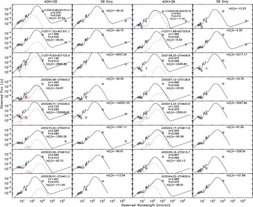
Observed frame best-fitting AGN+SB and SB-only SEDs to AzTEC/X-ray sources. The plots show the template models that lie closest to the best-fitting parameters determined from the MCMC SED fitting. The AGN and SB models are given by the dotted red and dashed blue lines, respectively, with their linear combination shown by the solid black line. Also shown for each source is the redshift used in the SED fitting, favouring the spectroscopic redshift where available, and the resulting best-fitting ln(L) values. For reference, we have included the probability of random association P (Table 1) for each source.

Figure 3

Open in new tab Download slide

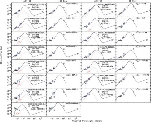
– continued

Table 5.

Best-fitting SED parameters using only the SB models. The SED-derived X-ray luminosity is left as a free parameter and provides no additional constraint to the SED fitting. Errors are given at the 1σ confidence level after marginalizing over all other free parameters in the fitted templates. Column 1: Chandra Source ID. Columns 2, 3 and 4: SB template normalization, age and optical depth. Column 5: total model-derived, rest-frame bolometric IR luminosity from ∼0.001–1500 μm. Column 6: SFR derived from equation (2) (Section 3.2.1) and Columns 2 and 3. Column 7: SED-derived X-ray luminosity. Column 8: fractional contribution of model to observed 1.1 mm flux. Column 9: ln(L) of best-fitting parameters.

Chandra ID	Norm	AGE	τ_ν	IR lum.	SFR	X-ray Lum.	f_1.1 mm	ln(L)
		(Myr)		(10¹² L_⊙)	(M_⊙ yr⁻¹)	(10⁴³ erg s⁻¹)
(1)	(2)	(3)	(4)	(5)	(6)	(7)	(8)	(9)
J123616.08+621514.1	7874.8\|$ {^{+ 261.8}_{-247.1}} $\|	45.2\|$ {^{+ 9.8}_{-6.9}} $\|	150.0\|$ {^{+ 41.5}_{-41.5}} $\|	9.87\|$ {^{+ 2.43}_{-2.47}} $\|	822	0.10\|$ {^{+ 0.03}_{-0.03}} $\|	1.22	−48.42
J123635.86+620707.8	246.9\|$ {^{+ 88.3}_{-81.7}} $\|	45.2\|$ {^{+ 26.8}_{-12.9}} $\|	199.4\|$ {^{+ 0.6}_{-88.3}} $\|	0.31\|$ {^{+ 0.19}_{-0.19}} $\|	26	0.00\|$ {^{+ 0.01}_{-0.01}} $\|	0.04	−12.25
J123711.32+621331.1	8412.4\|$ {^{+ 156.2}_{-184.8}} $\|	56.9\|$ {^{+ 6.1}_{-9.9}} $\|	199.0\|$ {^{+ 1.0}_{-41.1}} $\|	7.41\|$ {^{+ 2.63}_{-1.17}} $\|	489	0.08\|$ {^{+ 0.03}_{-0.01}} $\|	0.81	−28.15
J123711.98+621325.8	2832.8\|$ {^{+ 138.5}_{-625.4}} $\|	45.2\|$ {^{+ 10.0}_{-7.0}} $\|	199.6\|$ {^{+ 0.4}_{-48.2}} $\|	3.55\|$ {^{+ 0.91}_{-0.92}} $\|	296	0.04\|$ {^{+ 0.01}_{-0.01}} $\|	0.30	−9.35
J123716.63+621733.4	6318.3\|$ {^{+ 67.8}_{-66.2}} $\|	36.8\|$ {^{+ 6.9}_{-9.2}} $\|	200.0\|$ {^{+ 0.0}_{-42.2}} $\|	10.30\|$ {^{+ 3.30}_{-1.90}} $\|	1003	0.12\|$ {^{+ 0.04}_{-0.03}} $\|	1.14	−6057.59
J033158.25−274458.8	1123.2\|$ {^{+ 3.4}_{-2.3}} $\|	72.0\|$ {^{+ 0.0}_{-6.9}} $\|	199.8\|$ {^{+ 0.2}_{-43.2}} $\|	0.66\|$ {^{+ 0.13}_{-0.01}} $\|	31	0.01\|$ {^{+ 0.01}_{-0.01}} $\|	0.29	−2217.17
J033204.48−274643.3	302.8\|$ {^{+ 57.6}_{-62.5}} $\|	71.9\|$ {^{+ 0.1}_{-9.7}} $\|	101.1\|$ {^{+ 86.4}_{-51.1}} $\|	0.18\|$ {^{+ 0.06}_{-0.04}} $\|	8	0.00\|$ {^{+ 0.01}_{-0.01}} $\|	0.03	−26.34
J033207.12−275128.6	253.3\|$ {^{+ 14.9}_{-20.3}} $\|	71.8\|$ {^{+ 0.2}_{-12.9}} $\|	198.9\|$ {^{+ 1.1}_{-45.1}} $\|	0.15\|$ {^{+ 0.06}_{-0.01}} $\|	7	0.00\|$ {^{+ 0.01}_{-0.01}} $\|	0.03	−23.76
J033209.71−274249.0	2277.2\|$ {^{+ 3.4}_{-3.4}} $\|	71.9\|$ {^{+ 0.1}_{-6.8}} $\|	200.0\|$ {^{+ 0.0}_{-43.2}} $\|	1.33\|$ {^{+ 0.26}_{-0.01}} $\|	63	0.01\|$ {^{+ 0.01}_{-0.01}} $\|	0.72	−140 057.35
J033212.23−274620.9	2486.3\|$ {^{+ 6.3}_{-6.7}} $\|	71.9\|$ {^{+ 0.1}_{-6.8}} $\|	199.6\|$ {^{+ 0.4}_{-42.2}} $\|	1.45\|$ {^{+ 0.29}_{-0.01}} $\|	68	0.01\|$ {^{+ 0.01}_{-0.01}} $\|	0.36	−5567.86
J033215.32−275037.6	3491.2\|$ {^{+ 19.6}_{-20.2}} $\|	71.8\|$ {^{+ 0.2}_{-6.8}} $\|	50.1\|$ {^{+ 43.4}_{-0.1}} $\|	2.05\|$ {^{+ 0.40}_{-0.02}} $\|	96	0.01\|$ {^{+ 0.01}_{-0.01}} $\|	0.42	−1261.17
J033222.17−274811.6	2799.0\|$ {^{+ 20.3}_{-21.8}} $\|	45.4\|$ {^{+ 9.9}_{-7.2}} $\|	50.1\|$ {^{+ 42.1}_{-0.1}} $\|	3.49\|$ {^{+ 0.89}_{-0.88}} $\|	289	0.03\|$ {^{+ 0.01}_{-0.01}} $\|	0.49	−91.65
J033222.56−274815.0	4147.3\|$ {^{+ 24.7}_{-26.2}} $\|	72.0\|$ {^{+ 0.0}_{-6.9}} $\|	50.7\|$ {^{+ 42.5}_{-0.7}} $\|	2.42\|$ {^{+ 0.49}_{-0.01}} $\|	113	0.02\|$ {^{+ 0.01}_{-0.01}} $\|	0.58	−69.91
J033235.18−275215.7	109.1\|$ {^{+ 4.3}_{-14.4}} $\|	57.0\|$ {^{+ 6.2}_{-10.8}} $\|	198.8\|$ {^{+ 1.2}_{-90.5}} $\|	0.10\|$ {^{+ 0.04}_{-0.02}} $\|	6	0.00\|$ {^{+ 0.01}_{-0.01}} $\|	0.02	−328.50
J033238.01−274401.2	1069.4\|$ {^{+ 19.2}_{-17.5}} $\|	37.1\|$ {^{+ 6.6}_{-9.5}} $\|	199.9\|$ {^{+ 0.1}_{-43.0}} $\|	1.72\|$ {^{+ 0.57}_{-0.32}} $\|	167	0.02\|$ {^{+ 0.01}_{-0.01}} $\|	0.21	−112.10
J033244.02−274635.9	3419.4\|$ {^{+ 38.9}_{-37.5}} $\|	45.2\|$ {^{+ 9.9}_{-6.8}} $\|	101.1\|$ {^{+ 40.9}_{-41.8}} $\|	4.29\|$ {^{+ 1.03}_{-1.07}} $\|	357	0.04\|$ {^{+ 0.01}_{-0.01}} $\|	0.57	−101.89
J033246.83−275120.9	917.1\|$ {^{+ 6.7}_{-7.4}} $\|	71.8\|$ {^{+ 0.2}_{-6.7}} $\|	199.9\|$ {^{+ 0.1}_{-43.3}} $\|	0.54\|$ {^{+ 0.10}_{-0.01}} $\|	25	0.01\|$ {^{+ 0.01}_{-0.01}} $\|	0.22	−4061.23
J033302.94−275146.9	14 138.5\|$ {^{+ 225.5}_{-262.1}} $\|	37.0\|$ {^{+ 6.6}_{-9.3}} $\|	99.6\|$ {^{+ 42.0}_{-41.6}} $\|	22.80\|$ {^{+ 7.40}_{-4.20}} $\|	2223	0.23\|$ {^{+ 0.08}_{-0.05}} $\|	2.56	−65.28
J095905.05+022156.4	9410.8\|$ {^{+ 175.9}_{-193.1}} $\|	45.1\|$ {^{+ 9.9}_{-6.6}} $\|	150.7\|$ {^{+ 41.5}_{-42.4}} $\|	11.80\|$ {^{+ 2.80}_{-3.00}} $\|	987	0.13\|$ {^{+ 0.03}_{-0.04}} $\|	1.01	−4.61
J095929.70+021706.4	5070.1\|$ {^{+ 51.2}_{-211.0}} $\|	72.0\|$ {^{+ 0.1}_{-13.7}} $\|	150.4\|$ {^{+ 45.5}_{-47.6}} $\|	2.96\|$ {^{+ 1.19}_{-0.02}} $\|	139	0.03\|$ {^{+ 0.01}_{-0.01}} $\|	0.44	−2.47
J095945.15+023021.1	2282.0\|$ {^{+ 10.1}_{-9.9}} $\|	71.9\|$ {^{+ 0.1}_{-6.7}} $\|	100.1\|$ {^{+ 41.6}_{-41.4}} $\|	1.34\|$ {^{+ 0.26}_{-0.01}} $\|	63	0.01\|$ {^{+ 0.01}_{-0.01}} $\|	0.18	−706.44
J095953.85+021853.6	1705.2\|$ {^{+ 11.1}_{-10.2}} $\|	64.2\|$ {^{+ 6.6}_{-6.1}} $\|	199.8\|$ {^{+ 0.2}_{-42.7}} $\|	1.22\|$ {^{+ 0.23}_{-0.19}} $\|	69	0.01\|$ {^{+ 0.01}_{-0.01}} $\|	0.15	−297.44
J095959.96+020633.1	691.2\|$ {^{+ 5.4}_{-5.3}} $\|	45.2\|$ {^{+ 9.9}_{-7.1}} $\|	199.8\|$ {^{+ 0.2}_{-42.7}} $\|	0.87\|$ {^{+ 0.22}_{-0.22}} $\|	72	0.01\|$ {^{+ 0.01}_{-0.01}} $\|	0.08	−173.25
J100003.73+020206.4	1049.4\|$ {^{+ 31.6}_{-80.1}} $\|	71.9\|$ {^{+ 0.1}_{-22.6}} $\|	50.3\|$ {^{+ 42.8}_{-0.3}} $\|	0.62\|$ {^{+ 0.50}_{-0.02}} $\|	29	0.00\|$ {^{+ 0.01}_{-0.01}} $\|	0.07	−21.81
J100006.11+015239.2	3076.4\|$ {^{+ 31.8}_{-82.1}} $\|	71.8\|$ {^{+ 0.2}_{-13.1}} $\|	199.5\|$ {^{+ 0.5}_{-45.4}} $\|	1.81\|$ {^{+ 0.72}_{-0.03}} $\|	85	0.02\|$ {^{+ 0.01}_{-0.01}} $\|	0.24	−11.02
J100006.55+023259.3	2005.4\|$ {^{+ 13.9}_{-15.9}} $\|	72.0\|$ {^{+ 0.1}_{-6.8}} $\|	199.9\|$ {^{+ 0.1}_{-43.4}} $\|	1.17\|$ {^{+ 0.23}_{-0.01}} $\|	55	0.01\|$ {^{+ 0.01}_{-0.01}} $\|	0.15	−4308.82
J100033.61+014902.0	2553.0\|$ {^{+ 30.1}_{-26.7}} $\|	71.9\|$ {^{+ 0.1}_{-6.8}} $\|	200.0\|$ {^{+ 0.1}_{-42.9}} $\|	1.49\|$ {^{+ 0.29}_{-0.02}} $\|	70	0.02\|$ {^{+ 0.01}_{-0.01}} $\|	0.19	−327.48
J100055.34+023441.1	20 213.0\|$ {^{+ 53.9}_{-59.2}} $\|	36.8\|$ {^{+ 6.9}_{-9.0}} $\|	199.7\|$ {^{+ 0.3}_{-41.9}} $\|	32.90\|$ {^{+ 10.20}_{-6.20}} $\|	3210	0.38\|$ {^{+ 0.12}_{-0.08}} $\|	1.52	−10 787.79
J100107.46+015718.1	12 755.5\|$ {^{+ 126.0}_{-141.9}} $\|	26.1\|$ {^{+ 9.2}_{-8.5}} $\|	199.6\|$ {^{+ 0.4}_{-42.0}} $\|	28.40\|$ {^{+ 7.10}_{-6.60}} $\|	3459	0.33\|$ {^{+ 0.08}_{-0.08}} $\|	1.48	−8393.19
J100116.15+023606.9	6042.4\|$ {^{+ 14.7}_{-16.6}} $\|	45.0\|$ {^{+ 10.2}_{-6.7}} $\|	199.9\|$ {^{+ 0.1}_{-42.6}} $\|	7.62\|$ {^{+ 1.80}_{-1.97}} $\|	637	0.09\|$ {^{+ 0.02}_{-0.02}} $\|	0.61	−1990.78
J100139.73+022548.5	70.0\|$ {^{+ 0.5}_{-0.5}} $\|	71.9\|$ {^{+ 0.1}_{-6.9}} $\|	198.9\|$ {^{+ 1.1}_{-42.7}} $\|	0.04\|$ {^{+ 0.01}_{-0.01}} $\|	2	0.00\|$ {^{+ 0.01}_{-0.01}} $\|	0.06	−189 839.12

Chandra ID	Norm	AGE	τ_ν	IR lum.	SFR	X-ray Lum.	f_1.1 mm	ln(L)
		(Myr)		(10¹² L_⊙)	(M_⊙ yr⁻¹)	(10⁴³ erg s⁻¹)
(1)	(2)	(3)	(4)	(5)	(6)	(7)	(8)	(9)
J123616.08+621514.1	7874.8\|$ {^{+ 261.8}_{-247.1}} $\|	45.2\|$ {^{+ 9.8}_{-6.9}} $\|	150.0\|$ {^{+ 41.5}_{-41.5}} $\|	9.87\|$ {^{+ 2.43}_{-2.47}} $\|	822	0.10\|$ {^{+ 0.03}_{-0.03}} $\|	1.22	−48.42
J123635.86+620707.8	246.9\|$ {^{+ 88.3}_{-81.7}} $\|	45.2\|$ {^{+ 26.8}_{-12.9}} $\|	199.4\|$ {^{+ 0.6}_{-88.3}} $\|	0.31\|$ {^{+ 0.19}_{-0.19}} $\|	26	0.00\|$ {^{+ 0.01}_{-0.01}} $\|	0.04	−12.25
J123711.32+621331.1	8412.4\|$ {^{+ 156.2}_{-184.8}} $\|	56.9\|$ {^{+ 6.1}_{-9.9}} $\|	199.0\|$ {^{+ 1.0}_{-41.1}} $\|	7.41\|$ {^{+ 2.63}_{-1.17}} $\|	489	0.08\|$ {^{+ 0.03}_{-0.01}} $\|	0.81	−28.15
J123711.98+621325.8	2832.8\|$ {^{+ 138.5}_{-625.4}} $\|	45.2\|$ {^{+ 10.0}_{-7.0}} $\|	199.6\|$ {^{+ 0.4}_{-48.2}} $\|	3.55\|$ {^{+ 0.91}_{-0.92}} $\|	296	0.04\|$ {^{+ 0.01}_{-0.01}} $\|	0.30	−9.35
J123716.63+621733.4	6318.3\|$ {^{+ 67.8}_{-66.2}} $\|	36.8\|$ {^{+ 6.9}_{-9.2}} $\|	200.0\|$ {^{+ 0.0}_{-42.2}} $\|	10.30\|$ {^{+ 3.30}_{-1.90}} $\|	1003	0.12\|$ {^{+ 0.04}_{-0.03}} $\|	1.14	−6057.59
J033158.25−274458.8	1123.2\|$ {^{+ 3.4}_{-2.3}} $\|	72.0\|$ {^{+ 0.0}_{-6.9}} $\|	199.8\|$ {^{+ 0.2}_{-43.2}} $\|	0.66\|$ {^{+ 0.13}_{-0.01}} $\|	31	0.01\|$ {^{+ 0.01}_{-0.01}} $\|	0.29	−2217.17
J033204.48−274643.3	302.8\|$ {^{+ 57.6}_{-62.5}} $\|	71.9\|$ {^{+ 0.1}_{-9.7}} $\|	101.1\|$ {^{+ 86.4}_{-51.1}} $\|	0.18\|$ {^{+ 0.06}_{-0.04}} $\|	8	0.00\|$ {^{+ 0.01}_{-0.01}} $\|	0.03	−26.34
J033207.12−275128.6	253.3\|$ {^{+ 14.9}_{-20.3}} $\|	71.8\|$ {^{+ 0.2}_{-12.9}} $\|	198.9\|$ {^{+ 1.1}_{-45.1}} $\|	0.15\|$ {^{+ 0.06}_{-0.01}} $\|	7	0.00\|$ {^{+ 0.01}_{-0.01}} $\|	0.03	−23.76
J033209.71−274249.0	2277.2\|$ {^{+ 3.4}_{-3.4}} $\|	71.9\|$ {^{+ 0.1}_{-6.8}} $\|	200.0\|$ {^{+ 0.0}_{-43.2}} $\|	1.33\|$ {^{+ 0.26}_{-0.01}} $\|	63	0.01\|$ {^{+ 0.01}_{-0.01}} $\|	0.72	−140 057.35
J033212.23−274620.9	2486.3\|$ {^{+ 6.3}_{-6.7}} $\|	71.9\|$ {^{+ 0.1}_{-6.8}} $\|	199.6\|$ {^{+ 0.4}_{-42.2}} $\|	1.45\|$ {^{+ 0.29}_{-0.01}} $\|	68	0.01\|$ {^{+ 0.01}_{-0.01}} $\|	0.36	−5567.86
J033215.32−275037.6	3491.2\|$ {^{+ 19.6}_{-20.2}} $\|	71.8\|$ {^{+ 0.2}_{-6.8}} $\|	50.1\|$ {^{+ 43.4}_{-0.1}} $\|	2.05\|$ {^{+ 0.40}_{-0.02}} $\|	96	0.01\|$ {^{+ 0.01}_{-0.01}} $\|	0.42	−1261.17
J033222.17−274811.6	2799.0\|$ {^{+ 20.3}_{-21.8}} $\|	45.4\|$ {^{+ 9.9}_{-7.2}} $\|	50.1\|$ {^{+ 42.1}_{-0.1}} $\|	3.49\|$ {^{+ 0.89}_{-0.88}} $\|	289	0.03\|$ {^{+ 0.01}_{-0.01}} $\|	0.49	−91.65
J033222.56−274815.0	4147.3\|$ {^{+ 24.7}_{-26.2}} $\|	72.0\|$ {^{+ 0.0}_{-6.9}} $\|	50.7\|$ {^{+ 42.5}_{-0.7}} $\|	2.42\|$ {^{+ 0.49}_{-0.01}} $\|	113	0.02\|$ {^{+ 0.01}_{-0.01}} $\|	0.58	−69.91
J033235.18−275215.7	109.1\|$ {^{+ 4.3}_{-14.4}} $\|	57.0\|$ {^{+ 6.2}_{-10.8}} $\|	198.8\|$ {^{+ 1.2}_{-90.5}} $\|	0.10\|$ {^{+ 0.04}_{-0.02}} $\|	6	0.00\|$ {^{+ 0.01}_{-0.01}} $\|	0.02	−328.50
J033238.01−274401.2	1069.4\|$ {^{+ 19.2}_{-17.5}} $\|	37.1\|$ {^{+ 6.6}_{-9.5}} $\|	199.9\|$ {^{+ 0.1}_{-43.0}} $\|	1.72\|$ {^{+ 0.57}_{-0.32}} $\|	167	0.02\|$ {^{+ 0.01}_{-0.01}} $\|	0.21	−112.10
J033244.02−274635.9	3419.4\|$ {^{+ 38.9}_{-37.5}} $\|	45.2\|$ {^{+ 9.9}_{-6.8}} $\|	101.1\|$ {^{+ 40.9}_{-41.8}} $\|	4.29\|$ {^{+ 1.03}_{-1.07}} $\|	357	0.04\|$ {^{+ 0.01}_{-0.01}} $\|	0.57	−101.89
J033246.83−275120.9	917.1\|$ {^{+ 6.7}_{-7.4}} $\|	71.8\|$ {^{+ 0.2}_{-6.7}} $\|	199.9\|$ {^{+ 0.1}_{-43.3}} $\|	0.54\|$ {^{+ 0.10}_{-0.01}} $\|	25	0.01\|$ {^{+ 0.01}_{-0.01}} $\|	0.22	−4061.23
J033302.94−275146.9	14 138.5\|$ {^{+ 225.5}_{-262.1}} $\|	37.0\|$ {^{+ 6.6}_{-9.3}} $\|	99.6\|$ {^{+ 42.0}_{-41.6}} $\|	22.80\|$ {^{+ 7.40}_{-4.20}} $\|	2223	0.23\|$ {^{+ 0.08}_{-0.05}} $\|	2.56	−65.28
J095905.05+022156.4	9410.8\|$ {^{+ 175.9}_{-193.1}} $\|	45.1\|$ {^{+ 9.9}_{-6.6}} $\|	150.7\|$ {^{+ 41.5}_{-42.4}} $\|	11.80\|$ {^{+ 2.80}_{-3.00}} $\|	987	0.13\|$ {^{+ 0.03}_{-0.04}} $\|	1.01	−4.61
J095929.70+021706.4	5070.1\|$ {^{+ 51.2}_{-211.0}} $\|	72.0\|$ {^{+ 0.1}_{-13.7}} $\|	150.4\|$ {^{+ 45.5}_{-47.6}} $\|	2.96\|$ {^{+ 1.19}_{-0.02}} $\|	139	0.03\|$ {^{+ 0.01}_{-0.01}} $\|	0.44	−2.47
J095945.15+023021.1	2282.0\|$ {^{+ 10.1}_{-9.9}} $\|	71.9\|$ {^{+ 0.1}_{-6.7}} $\|	100.1\|$ {^{+ 41.6}_{-41.4}} $\|	1.34\|$ {^{+ 0.26}_{-0.01}} $\|	63	0.01\|$ {^{+ 0.01}_{-0.01}} $\|	0.18	−706.44
J095953.85+021853.6	1705.2\|$ {^{+ 11.1}_{-10.2}} $\|	64.2\|$ {^{+ 6.6}_{-6.1}} $\|	199.8\|$ {^{+ 0.2}_{-42.7}} $\|	1.22\|$ {^{+ 0.23}_{-0.19}} $\|	69	0.01\|$ {^{+ 0.01}_{-0.01}} $\|	0.15	−297.44
J095959.96+020633.1	691.2\|$ {^{+ 5.4}_{-5.3}} $\|	45.2\|$ {^{+ 9.9}_{-7.1}} $\|	199.8\|$ {^{+ 0.2}_{-42.7}} $\|	0.87\|$ {^{+ 0.22}_{-0.22}} $\|	72	0.01\|$ {^{+ 0.01}_{-0.01}} $\|	0.08	−173.25
J100003.73+020206.4	1049.4\|$ {^{+ 31.6}_{-80.1}} $\|	71.9\|$ {^{+ 0.1}_{-22.6}} $\|	50.3\|$ {^{+ 42.8}_{-0.3}} $\|	0.62\|$ {^{+ 0.50}_{-0.02}} $\|	29	0.00\|$ {^{+ 0.01}_{-0.01}} $\|	0.07	−21.81
J100006.11+015239.2	3076.4\|$ {^{+ 31.8}_{-82.1}} $\|	71.8\|$ {^{+ 0.2}_{-13.1}} $\|	199.5\|$ {^{+ 0.5}_{-45.4}} $\|	1.81\|$ {^{+ 0.72}_{-0.03}} $\|	85	0.02\|$ {^{+ 0.01}_{-0.01}} $\|	0.24	−11.02
J100006.55+023259.3	2005.4\|$ {^{+ 13.9}_{-15.9}} $\|	72.0\|$ {^{+ 0.1}_{-6.8}} $\|	199.9\|$ {^{+ 0.1}_{-43.4}} $\|	1.17\|$ {^{+ 0.23}_{-0.01}} $\|	55	0.01\|$ {^{+ 0.01}_{-0.01}} $\|	0.15	−4308.82
J100033.61+014902.0	2553.0\|$ {^{+ 30.1}_{-26.7}} $\|	71.9\|$ {^{+ 0.1}_{-6.8}} $\|	200.0\|$ {^{+ 0.1}_{-42.9}} $\|	1.49\|$ {^{+ 0.29}_{-0.02}} $\|	70	0.02\|$ {^{+ 0.01}_{-0.01}} $\|	0.19	−327.48
J100055.34+023441.1	20 213.0\|$ {^{+ 53.9}_{-59.2}} $\|	36.8\|$ {^{+ 6.9}_{-9.0}} $\|	199.7\|$ {^{+ 0.3}_{-41.9}} $\|	32.90\|$ {^{+ 10.20}_{-6.20}} $\|	3210	0.38\|$ {^{+ 0.12}_{-0.08}} $\|	1.52	−10 787.79
J100107.46+015718.1	12 755.5\|$ {^{+ 126.0}_{-141.9}} $\|	26.1\|$ {^{+ 9.2}_{-8.5}} $\|	199.6\|$ {^{+ 0.4}_{-42.0}} $\|	28.40\|$ {^{+ 7.10}_{-6.60}} $\|	3459	0.33\|$ {^{+ 0.08}_{-0.08}} $\|	1.48	−8393.19
J100116.15+023606.9	6042.4\|$ {^{+ 14.7}_{-16.6}} $\|	45.0\|$ {^{+ 10.2}_{-6.7}} $\|	199.9\|$ {^{+ 0.1}_{-42.6}} $\|	7.62\|$ {^{+ 1.80}_{-1.97}} $\|	637	0.09\|$ {^{+ 0.02}_{-0.02}} $\|	0.61	−1990.78
J100139.73+022548.5	70.0\|$ {^{+ 0.5}_{-0.5}} $\|	71.9\|$ {^{+ 0.1}_{-6.9}} $\|	198.9\|$ {^{+ 1.1}_{-42.7}} $\|	0.04\|$ {^{+ 0.01}_{-0.01}} $\|	2	0.00\|$ {^{+ 0.01}_{-0.01}} $\|	0.06	−189 839.12

Open in new tab

Table 5.

Best-fitting SED parameters using only the SB models. The SED-derived X-ray luminosity is left as a free parameter and provides no additional constraint to the SED fitting. Errors are given at the 1σ confidence level after marginalizing over all other free parameters in the fitted templates. Column 1: Chandra Source ID. Columns 2, 3 and 4: SB template normalization, age and optical depth. Column 5: total model-derived, rest-frame bolometric IR luminosity from ∼0.001–1500 μm. Column 6: SFR derived from equation (2) (Section 3.2.1) and Columns 2 and 3. Column 7: SED-derived X-ray luminosity. Column 8: fractional contribution of model to observed 1.1 mm flux. Column 9: ln(L) of best-fitting parameters.

Chandra ID	Norm	AGE	τ_ν	IR lum.	SFR	X-ray Lum.	f_1.1 mm	ln(L)
		(Myr)		(10¹² L_⊙)	(M_⊙ yr⁻¹)	(10⁴³ erg s⁻¹)
(1)	(2)	(3)	(4)	(5)	(6)	(7)	(8)	(9)
J123616.08+621514.1	7874.8\|$ {^{+ 261.8}_{-247.1}} $\|	45.2\|$ {^{+ 9.8}_{-6.9}} $\|	150.0\|$ {^{+ 41.5}_{-41.5}} $\|	9.87\|$ {^{+ 2.43}_{-2.47}} $\|	822	0.10\|$ {^{+ 0.03}_{-0.03}} $\|	1.22	−48.42
J123635.86+620707.8	246.9\|$ {^{+ 88.3}_{-81.7}} $\|	45.2\|$ {^{+ 26.8}_{-12.9}} $\|	199.4\|$ {^{+ 0.6}_{-88.3}} $\|	0.31\|$ {^{+ 0.19}_{-0.19}} $\|	26	0.00\|$ {^{+ 0.01}_{-0.01}} $\|	0.04	−12.25
J123711.32+621331.1	8412.4\|$ {^{+ 156.2}_{-184.8}} $\|	56.9\|$ {^{+ 6.1}_{-9.9}} $\|	199.0\|$ {^{+ 1.0}_{-41.1}} $\|	7.41\|$ {^{+ 2.63}_{-1.17}} $\|	489	0.08\|$ {^{+ 0.03}_{-0.01}} $\|	0.81	−28.15
J123711.98+621325.8	2832.8\|$ {^{+ 138.5}_{-625.4}} $\|	45.2\|$ {^{+ 10.0}_{-7.0}} $\|	199.6\|$ {^{+ 0.4}_{-48.2}} $\|	3.55\|$ {^{+ 0.91}_{-0.92}} $\|	296	0.04\|$ {^{+ 0.01}_{-0.01}} $\|	0.30	−9.35
J123716.63+621733.4	6318.3\|$ {^{+ 67.8}_{-66.2}} $\|	36.8\|$ {^{+ 6.9}_{-9.2}} $\|	200.0\|$ {^{+ 0.0}_{-42.2}} $\|	10.30\|$ {^{+ 3.30}_{-1.90}} $\|	1003	0.12\|$ {^{+ 0.04}_{-0.03}} $\|	1.14	−6057.59
J033158.25−274458.8	1123.2\|$ {^{+ 3.4}_{-2.3}} $\|	72.0\|$ {^{+ 0.0}_{-6.9}} $\|	199.8\|$ {^{+ 0.2}_{-43.2}} $\|	0.66\|$ {^{+ 0.13}_{-0.01}} $\|	31	0.01\|$ {^{+ 0.01}_{-0.01}} $\|	0.29	−2217.17
J033204.48−274643.3	302.8\|$ {^{+ 57.6}_{-62.5}} $\|	71.9\|$ {^{+ 0.1}_{-9.7}} $\|	101.1\|$ {^{+ 86.4}_{-51.1}} $\|	0.18\|$ {^{+ 0.06}_{-0.04}} $\|	8	0.00\|$ {^{+ 0.01}_{-0.01}} $\|	0.03	−26.34
J033207.12−275128.6	253.3\|$ {^{+ 14.9}_{-20.3}} $\|	71.8\|$ {^{+ 0.2}_{-12.9}} $\|	198.9\|$ {^{+ 1.1}_{-45.1}} $\|	0.15\|$ {^{+ 0.06}_{-0.01}} $\|	7	0.00\|$ {^{+ 0.01}_{-0.01}} $\|	0.03	−23.76
J033209.71−274249.0	2277.2\|$ {^{+ 3.4}_{-3.4}} $\|	71.9\|$ {^{+ 0.1}_{-6.8}} $\|	200.0\|$ {^{+ 0.0}_{-43.2}} $\|	1.33\|$ {^{+ 0.26}_{-0.01}} $\|	63	0.01\|$ {^{+ 0.01}_{-0.01}} $\|	0.72	−140 057.35
J033212.23−274620.9	2486.3\|$ {^{+ 6.3}_{-6.7}} $\|	71.9\|$ {^{+ 0.1}_{-6.8}} $\|	199.6\|$ {^{+ 0.4}_{-42.2}} $\|	1.45\|$ {^{+ 0.29}_{-0.01}} $\|	68	0.01\|$ {^{+ 0.01}_{-0.01}} $\|	0.36	−5567.86
J033215.32−275037.6	3491.2\|$ {^{+ 19.6}_{-20.2}} $\|	71.8\|$ {^{+ 0.2}_{-6.8}} $\|	50.1\|$ {^{+ 43.4}_{-0.1}} $\|	2.05\|$ {^{+ 0.40}_{-0.02}} $\|	96	0.01\|$ {^{+ 0.01}_{-0.01}} $\|	0.42	−1261.17
J033222.17−274811.6	2799.0\|$ {^{+ 20.3}_{-21.8}} $\|	45.4\|$ {^{+ 9.9}_{-7.2}} $\|	50.1\|$ {^{+ 42.1}_{-0.1}} $\|	3.49\|$ {^{+ 0.89}_{-0.88}} $\|	289	0.03\|$ {^{+ 0.01}_{-0.01}} $\|	0.49	−91.65
J033222.56−274815.0	4147.3\|$ {^{+ 24.7}_{-26.2}} $\|	72.0\|$ {^{+ 0.0}_{-6.9}} $\|	50.7\|$ {^{+ 42.5}_{-0.7}} $\|	2.42\|$ {^{+ 0.49}_{-0.01}} $\|	113	0.02\|$ {^{+ 0.01}_{-0.01}} $\|	0.58	−69.91
J033235.18−275215.7	109.1\|$ {^{+ 4.3}_{-14.4}} $\|	57.0\|$ {^{+ 6.2}_{-10.8}} $\|	198.8\|$ {^{+ 1.2}_{-90.5}} $\|	0.10\|$ {^{+ 0.04}_{-0.02}} $\|	6	0.00\|$ {^{+ 0.01}_{-0.01}} $\|	0.02	−328.50
J033238.01−274401.2	1069.4\|$ {^{+ 19.2}_{-17.5}} $\|	37.1\|$ {^{+ 6.6}_{-9.5}} $\|	199.9\|$ {^{+ 0.1}_{-43.0}} $\|	1.72\|$ {^{+ 0.57}_{-0.32}} $\|	167	0.02\|$ {^{+ 0.01}_{-0.01}} $\|	0.21	−112.10
J033244.02−274635.9	3419.4\|$ {^{+ 38.9}_{-37.5}} $\|	45.2\|$ {^{+ 9.9}_{-6.8}} $\|	101.1\|$ {^{+ 40.9}_{-41.8}} $\|	4.29\|$ {^{+ 1.03}_{-1.07}} $\|	357	0.04\|$ {^{+ 0.01}_{-0.01}} $\|	0.57	−101.89
J033246.83−275120.9	917.1\|$ {^{+ 6.7}_{-7.4}} $\|	71.8\|$ {^{+ 0.2}_{-6.7}} $\|	199.9\|$ {^{+ 0.1}_{-43.3}} $\|	0.54\|$ {^{+ 0.10}_{-0.01}} $\|	25	0.01\|$ {^{+ 0.01}_{-0.01}} $\|	0.22	−4061.23
J033302.94−275146.9	14 138.5\|$ {^{+ 225.5}_{-262.1}} $\|	37.0\|$ {^{+ 6.6}_{-9.3}} $\|	99.6\|$ {^{+ 42.0}_{-41.6}} $\|	22.80\|$ {^{+ 7.40}_{-4.20}} $\|	2223	0.23\|$ {^{+ 0.08}_{-0.05}} $\|	2.56	−65.28
J095905.05+022156.4	9410.8\|$ {^{+ 175.9}_{-193.1}} $\|	45.1\|$ {^{+ 9.9}_{-6.6}} $\|	150.7\|$ {^{+ 41.5}_{-42.4}} $\|	11.80\|$ {^{+ 2.80}_{-3.00}} $\|	987	0.13\|$ {^{+ 0.03}_{-0.04}} $\|	1.01	−4.61
J095929.70+021706.4	5070.1\|$ {^{+ 51.2}_{-211.0}} $\|	72.0\|$ {^{+ 0.1}_{-13.7}} $\|	150.4\|$ {^{+ 45.5}_{-47.6}} $\|	2.96\|$ {^{+ 1.19}_{-0.02}} $\|	139	0.03\|$ {^{+ 0.01}_{-0.01}} $\|	0.44	−2.47
J095945.15+023021.1	2282.0\|$ {^{+ 10.1}_{-9.9}} $\|	71.9\|$ {^{+ 0.1}_{-6.7}} $\|	100.1\|$ {^{+ 41.6}_{-41.4}} $\|	1.34\|$ {^{+ 0.26}_{-0.01}} $\|	63	0.01\|$ {^{+ 0.01}_{-0.01}} $\|	0.18	−706.44
J095953.85+021853.6	1705.2\|$ {^{+ 11.1}_{-10.2}} $\|	64.2\|$ {^{+ 6.6}_{-6.1}} $\|	199.8\|$ {^{+ 0.2}_{-42.7}} $\|	1.22\|$ {^{+ 0.23}_{-0.19}} $\|	69	0.01\|$ {^{+ 0.01}_{-0.01}} $\|	0.15	−297.44
J095959.96+020633.1	691.2\|$ {^{+ 5.4}_{-5.3}} $\|	45.2\|$ {^{+ 9.9}_{-7.1}} $\|	199.8\|$ {^{+ 0.2}_{-42.7}} $\|	0.87\|$ {^{+ 0.22}_{-0.22}} $\|	72	0.01\|$ {^{+ 0.01}_{-0.01}} $\|	0.08	−173.25
J100003.73+020206.4	1049.4\|$ {^{+ 31.6}_{-80.1}} $\|	71.9\|$ {^{+ 0.1}_{-22.6}} $\|	50.3\|$ {^{+ 42.8}_{-0.3}} $\|	0.62\|$ {^{+ 0.50}_{-0.02}} $\|	29	0.00\|$ {^{+ 0.01}_{-0.01}} $\|	0.07	−21.81
J100006.11+015239.2	3076.4\|$ {^{+ 31.8}_{-82.1}} $\|	71.8\|$ {^{+ 0.2}_{-13.1}} $\|	199.5\|$ {^{+ 0.5}_{-45.4}} $\|	1.81\|$ {^{+ 0.72}_{-0.03}} $\|	85	0.02\|$ {^{+ 0.01}_{-0.01}} $\|	0.24	−11.02
J100006.55+023259.3	2005.4\|$ {^{+ 13.9}_{-15.9}} $\|	72.0\|$ {^{+ 0.1}_{-6.8}} $\|	199.9\|$ {^{+ 0.1}_{-43.4}} $\|	1.17\|$ {^{+ 0.23}_{-0.01}} $\|	55	0.01\|$ {^{+ 0.01}_{-0.01}} $\|	0.15	−4308.82
J100033.61+014902.0	2553.0\|$ {^{+ 30.1}_{-26.7}} $\|	71.9\|$ {^{+ 0.1}_{-6.8}} $\|	200.0\|$ {^{+ 0.1}_{-42.9}} $\|	1.49\|$ {^{+ 0.29}_{-0.02}} $\|	70	0.02\|$ {^{+ 0.01}_{-0.01}} $\|	0.19	−327.48
J100055.34+023441.1	20 213.0\|$ {^{+ 53.9}_{-59.2}} $\|	36.8\|$ {^{+ 6.9}_{-9.0}} $\|	199.7\|$ {^{+ 0.3}_{-41.9}} $\|	32.90\|$ {^{+ 10.20}_{-6.20}} $\|	3210	0.38\|$ {^{+ 0.12}_{-0.08}} $\|	1.52	−10 787.79
J100107.46+015718.1	12 755.5\|$ {^{+ 126.0}_{-141.9}} $\|	26.1\|$ {^{+ 9.2}_{-8.5}} $\|	199.6\|$ {^{+ 0.4}_{-42.0}} $\|	28.40\|$ {^{+ 7.10}_{-6.60}} $\|	3459	0.33\|$ {^{+ 0.08}_{-0.08}} $\|	1.48	−8393.19
J100116.15+023606.9	6042.4\|$ {^{+ 14.7}_{-16.6}} $\|	45.0\|$ {^{+ 10.2}_{-6.7}} $\|	199.9\|$ {^{+ 0.1}_{-42.6}} $\|	7.62\|$ {^{+ 1.80}_{-1.97}} $\|	637	0.09\|$ {^{+ 0.02}_{-0.02}} $\|	0.61	−1990.78
J100139.73+022548.5	70.0\|$ {^{+ 0.5}_{-0.5}} $\|	71.9\|$ {^{+ 0.1}_{-6.9}} $\|	198.9\|$ {^{+ 1.1}_{-42.7}} $\|	0.04\|$ {^{+ 0.01}_{-0.01}} $\|	2	0.00\|$ {^{+ 0.01}_{-0.01}} $\|	0.06	−189 839.12

Chandra ID	Norm	AGE	τ_ν	IR lum.	SFR	X-ray Lum.	f_1.1 mm	ln(L)
		(Myr)		(10¹² L_⊙)	(M_⊙ yr⁻¹)	(10⁴³ erg s⁻¹)
(1)	(2)	(3)	(4)	(5)	(6)	(7)	(8)	(9)
J123616.08+621514.1	7874.8\|$ {^{+ 261.8}_{-247.1}} $\|	45.2\|$ {^{+ 9.8}_{-6.9}} $\|	150.0\|$ {^{+ 41.5}_{-41.5}} $\|	9.87\|$ {^{+ 2.43}_{-2.47}} $\|	822	0.10\|$ {^{+ 0.03}_{-0.03}} $\|	1.22	−48.42
J123635.86+620707.8	246.9\|$ {^{+ 88.3}_{-81.7}} $\|	45.2\|$ {^{+ 26.8}_{-12.9}} $\|	199.4\|$ {^{+ 0.6}_{-88.3}} $\|	0.31\|$ {^{+ 0.19}_{-0.19}} $\|	26	0.00\|$ {^{+ 0.01}_{-0.01}} $\|	0.04	−12.25
J123711.32+621331.1	8412.4\|$ {^{+ 156.2}_{-184.8}} $\|	56.9\|$ {^{+ 6.1}_{-9.9}} $\|	199.0\|$ {^{+ 1.0}_{-41.1}} $\|	7.41\|$ {^{+ 2.63}_{-1.17}} $\|	489	0.08\|$ {^{+ 0.03}_{-0.01}} $\|	0.81	−28.15
J123711.98+621325.8	2832.8\|$ {^{+ 138.5}_{-625.4}} $\|	45.2\|$ {^{+ 10.0}_{-7.0}} $\|	199.6\|$ {^{+ 0.4}_{-48.2}} $\|	3.55\|$ {^{+ 0.91}_{-0.92}} $\|	296	0.04\|$ {^{+ 0.01}_{-0.01}} $\|	0.30	−9.35
J123716.63+621733.4	6318.3\|$ {^{+ 67.8}_{-66.2}} $\|	36.8\|$ {^{+ 6.9}_{-9.2}} $\|	200.0\|$ {^{+ 0.0}_{-42.2}} $\|	10.30\|$ {^{+ 3.30}_{-1.90}} $\|	1003	0.12\|$ {^{+ 0.04}_{-0.03}} $\|	1.14	−6057.59
J033158.25−274458.8	1123.2\|$ {^{+ 3.4}_{-2.3}} $\|	72.0\|$ {^{+ 0.0}_{-6.9}} $\|	199.8\|$ {^{+ 0.2}_{-43.2}} $\|	0.66\|$ {^{+ 0.13}_{-0.01}} $\|	31	0.01\|$ {^{+ 0.01}_{-0.01}} $\|	0.29	−2217.17
J033204.48−274643.3	302.8\|$ {^{+ 57.6}_{-62.5}} $\|	71.9\|$ {^{+ 0.1}_{-9.7}} $\|	101.1\|$ {^{+ 86.4}_{-51.1}} $\|	0.18\|$ {^{+ 0.06}_{-0.04}} $\|	8	0.00\|$ {^{+ 0.01}_{-0.01}} $\|	0.03	−26.34
J033207.12−275128.6	253.3\|$ {^{+ 14.9}_{-20.3}} $\|	71.8\|$ {^{+ 0.2}_{-12.9}} $\|	198.9\|$ {^{+ 1.1}_{-45.1}} $\|	0.15\|$ {^{+ 0.06}_{-0.01}} $\|	7	0.00\|$ {^{+ 0.01}_{-0.01}} $\|	0.03	−23.76
J033209.71−274249.0	2277.2\|$ {^{+ 3.4}_{-3.4}} $\|	71.9\|$ {^{+ 0.1}_{-6.8}} $\|	200.0\|$ {^{+ 0.0}_{-43.2}} $\|	1.33\|$ {^{+ 0.26}_{-0.01}} $\|	63	0.01\|$ {^{+ 0.01}_{-0.01}} $\|	0.72	−140 057.35
J033212.23−274620.9	2486.3\|$ {^{+ 6.3}_{-6.7}} $\|	71.9\|$ {^{+ 0.1}_{-6.8}} $\|	199.6\|$ {^{+ 0.4}_{-42.2}} $\|	1.45\|$ {^{+ 0.29}_{-0.01}} $\|	68	0.01\|$ {^{+ 0.01}_{-0.01}} $\|	0.36	−5567.86
J033215.32−275037.6	3491.2\|$ {^{+ 19.6}_{-20.2}} $\|	71.8\|$ {^{+ 0.2}_{-6.8}} $\|	50.1\|$ {^{+ 43.4}_{-0.1}} $\|	2.05\|$ {^{+ 0.40}_{-0.02}} $\|	96	0.01\|$ {^{+ 0.01}_{-0.01}} $\|	0.42	−1261.17
J033222.17−274811.6	2799.0\|$ {^{+ 20.3}_{-21.8}} $\|	45.4\|$ {^{+ 9.9}_{-7.2}} $\|	50.1\|$ {^{+ 42.1}_{-0.1}} $\|	3.49\|$ {^{+ 0.89}_{-0.88}} $\|	289	0.03\|$ {^{+ 0.01}_{-0.01}} $\|	0.49	−91.65
J033222.56−274815.0	4147.3\|$ {^{+ 24.7}_{-26.2}} $\|	72.0\|$ {^{+ 0.0}_{-6.9}} $\|	50.7\|$ {^{+ 42.5}_{-0.7}} $\|	2.42\|$ {^{+ 0.49}_{-0.01}} $\|	113	0.02\|$ {^{+ 0.01}_{-0.01}} $\|	0.58	−69.91
J033235.18−275215.7	109.1\|$ {^{+ 4.3}_{-14.4}} $\|	57.0\|$ {^{+ 6.2}_{-10.8}} $\|	198.8\|$ {^{+ 1.2}_{-90.5}} $\|	0.10\|$ {^{+ 0.04}_{-0.02}} $\|	6	0.00\|$ {^{+ 0.01}_{-0.01}} $\|	0.02	−328.50
J033238.01−274401.2	1069.4\|$ {^{+ 19.2}_{-17.5}} $\|	37.1\|$ {^{+ 6.6}_{-9.5}} $\|	199.9\|$ {^{+ 0.1}_{-43.0}} $\|	1.72\|$ {^{+ 0.57}_{-0.32}} $\|	167	0.02\|$ {^{+ 0.01}_{-0.01}} $\|	0.21	−112.10
J033244.02−274635.9	3419.4\|$ {^{+ 38.9}_{-37.5}} $\|	45.2\|$ {^{+ 9.9}_{-6.8}} $\|	101.1\|$ {^{+ 40.9}_{-41.8}} $\|	4.29\|$ {^{+ 1.03}_{-1.07}} $\|	357	0.04\|$ {^{+ 0.01}_{-0.01}} $\|	0.57	−101.89
J033246.83−275120.9	917.1\|$ {^{+ 6.7}_{-7.4}} $\|	71.8\|$ {^{+ 0.2}_{-6.7}} $\|	199.9\|$ {^{+ 0.1}_{-43.3}} $\|	0.54\|$ {^{+ 0.10}_{-0.01}} $\|	25	0.01\|$ {^{+ 0.01}_{-0.01}} $\|	0.22	−4061.23
J033302.94−275146.9	14 138.5\|$ {^{+ 225.5}_{-262.1}} $\|	37.0\|$ {^{+ 6.6}_{-9.3}} $\|	99.6\|$ {^{+ 42.0}_{-41.6}} $\|	22.80\|$ {^{+ 7.40}_{-4.20}} $\|	2223	0.23\|$ {^{+ 0.08}_{-0.05}} $\|	2.56	−65.28
J095905.05+022156.4	9410.8\|$ {^{+ 175.9}_{-193.1}} $\|	45.1\|$ {^{+ 9.9}_{-6.6}} $\|	150.7\|$ {^{+ 41.5}_{-42.4}} $\|	11.80\|$ {^{+ 2.80}_{-3.00}} $\|	987	0.13\|$ {^{+ 0.03}_{-0.04}} $\|	1.01	−4.61
J095929.70+021706.4	5070.1\|$ {^{+ 51.2}_{-211.0}} $\|	72.0\|$ {^{+ 0.1}_{-13.7}} $\|	150.4\|$ {^{+ 45.5}_{-47.6}} $\|	2.96\|$ {^{+ 1.19}_{-0.02}} $\|	139	0.03\|$ {^{+ 0.01}_{-0.01}} $\|	0.44	−2.47
J095945.15+023021.1	2282.0\|$ {^{+ 10.1}_{-9.9}} $\|	71.9\|$ {^{+ 0.1}_{-6.7}} $\|	100.1\|$ {^{+ 41.6}_{-41.4}} $\|	1.34\|$ {^{+ 0.26}_{-0.01}} $\|	63	0.01\|$ {^{+ 0.01}_{-0.01}} $\|	0.18	−706.44
J095953.85+021853.6	1705.2\|$ {^{+ 11.1}_{-10.2}} $\|	64.2\|$ {^{+ 6.6}_{-6.1}} $\|	199.8\|$ {^{+ 0.2}_{-42.7}} $\|	1.22\|$ {^{+ 0.23}_{-0.19}} $\|	69	0.01\|$ {^{+ 0.01}_{-0.01}} $\|	0.15	−297.44
J095959.96+020633.1	691.2\|$ {^{+ 5.4}_{-5.3}} $\|	45.2\|$ {^{+ 9.9}_{-7.1}} $\|	199.8\|$ {^{+ 0.2}_{-42.7}} $\|	0.87\|$ {^{+ 0.22}_{-0.22}} $\|	72	0.01\|$ {^{+ 0.01}_{-0.01}} $\|	0.08	−173.25
J100003.73+020206.4	1049.4\|$ {^{+ 31.6}_{-80.1}} $\|	71.9\|$ {^{+ 0.1}_{-22.6}} $\|	50.3\|$ {^{+ 42.8}_{-0.3}} $\|	0.62\|$ {^{+ 0.50}_{-0.02}} $\|	29	0.00\|$ {^{+ 0.01}_{-0.01}} $\|	0.07	−21.81
J100006.11+015239.2	3076.4\|$ {^{+ 31.8}_{-82.1}} $\|	71.8\|$ {^{+ 0.2}_{-13.1}} $\|	199.5\|$ {^{+ 0.5}_{-45.4}} $\|	1.81\|$ {^{+ 0.72}_{-0.03}} $\|	85	0.02\|$ {^{+ 0.01}_{-0.01}} $\|	0.24	−11.02
J100006.55+023259.3	2005.4\|$ {^{+ 13.9}_{-15.9}} $\|	72.0\|$ {^{+ 0.1}_{-6.8}} $\|	199.9\|$ {^{+ 0.1}_{-43.4}} $\|	1.17\|$ {^{+ 0.23}_{-0.01}} $\|	55	0.01\|$ {^{+ 0.01}_{-0.01}} $\|	0.15	−4308.82
J100033.61+014902.0	2553.0\|$ {^{+ 30.1}_{-26.7}} $\|	71.9\|$ {^{+ 0.1}_{-6.8}} $\|	200.0\|$ {^{+ 0.1}_{-42.9}} $\|	1.49\|$ {^{+ 0.29}_{-0.02}} $\|	70	0.02\|$ {^{+ 0.01}_{-0.01}} $\|	0.19	−327.48
J100055.34+023441.1	20 213.0\|$ {^{+ 53.9}_{-59.2}} $\|	36.8\|$ {^{+ 6.9}_{-9.0}} $\|	199.7\|$ {^{+ 0.3}_{-41.9}} $\|	32.90\|$ {^{+ 10.20}_{-6.20}} $\|	3210	0.38\|$ {^{+ 0.12}_{-0.08}} $\|	1.52	−10 787.79
J100107.46+015718.1	12 755.5\|$ {^{+ 126.0}_{-141.9}} $\|	26.1\|$ {^{+ 9.2}_{-8.5}} $\|	199.6\|$ {^{+ 0.4}_{-42.0}} $\|	28.40\|$ {^{+ 7.10}_{-6.60}} $\|	3459	0.33\|$ {^{+ 0.08}_{-0.08}} $\|	1.48	−8393.19
J100116.15+023606.9	6042.4\|$ {^{+ 14.7}_{-16.6}} $\|	45.0\|$ {^{+ 10.2}_{-6.7}} $\|	199.9\|$ {^{+ 0.1}_{-42.6}} $\|	7.62\|$ {^{+ 1.80}_{-1.97}} $\|	637	0.09\|$ {^{+ 0.02}_{-0.02}} $\|	0.61	−1990.78
J100139.73+022548.5	70.0\|$ {^{+ 0.5}_{-0.5}} $\|	71.9\|$ {^{+ 0.1}_{-6.9}} $\|	198.9\|$ {^{+ 1.1}_{-42.7}} $\|	0.04\|$ {^{+ 0.01}_{-0.01}} $\|	2	0.00\|$ {^{+ 0.01}_{-0.01}} $\|	0.06	−189 839.12

Open in new tab

SED fitting results

Fig. 3 shows that our method is able to produce reasonable fits to the AzTEC/X-ray sources; the source J033234.78−274815.0 was excluded as it has no discernible IRAC/MIPS counterpart despite having a spectroscopic redshift (see Table 2). While the majority (∼87 per cent) of our sources can be fitted using the SB templates alone, they typically underpredict the 1.1 mm emission, recovering on average ∼30–38 per cent of the observed flux. Including the AGN models helps to slightly increase the model fluxes, and the models are generally required to match the X-ray luminosity prior but are still unable to match the mm-wavelength observations, contributing little, if at all, to the bolometric luminosities and observed 1.1 mm flux. In some cases (e.g. J033212.23−274620.9), the AGN and SB templates appear very similar in the final fit. This likely results from the similarities in the dust treatment and radiative transfer in the templates as noted by Siebenmorgen & Efstathiou (2005) for effectively identical template parameters (i.e. dust content, optical depth and intrinsic luminosity; see also their fig. 4). In many cases, the fit values for AGN R and A_V are rather poor and show a large range in acceptable values. This effect stems from our use of the X-ray luminosity prior which effectively sets the AGN bolometric luminosity, preventing any additional AGN contribution to the bolometric SED and thus leading to unconstrained R and A_V (see also Fig. 5). The fact that A_V had such poor constraints prompted us to include the X-ray column density to avoid overestimating the dust content. By virtue of our MCMC technique, we may readily identify any degeneracies between the AGN and SB template sets; however, Fig. 4 shows that there are no large parameter–parameter degeneracies, although some parameters are not very well constrained. This is particularly the case for AGN R and A_V as mentioned above.

Figure 4.

Open in new tab Download slide

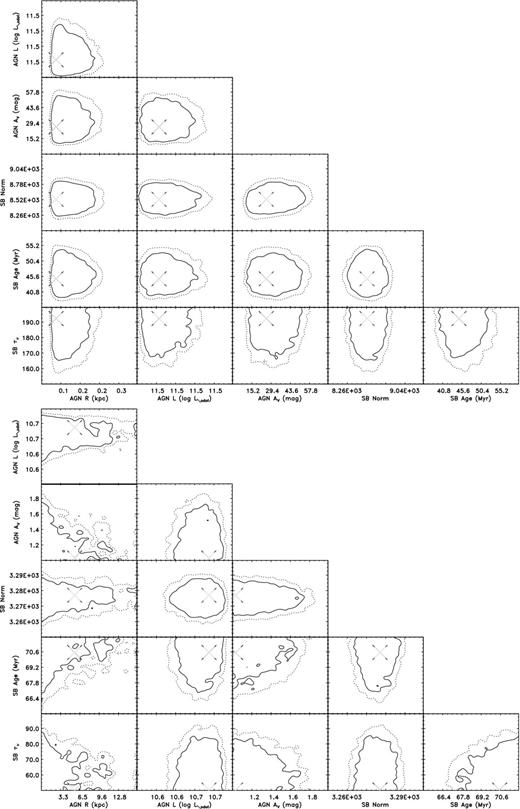
Smoothed, marginalized likelihood distribution of accepted parameter steps for J123616.08+621514.1 (top) and J033215.32−275037.6 (bottom), using the AGN+SB templates. A description of each parameter in the AGN and SB templates is given in Section 3.2.1. The location of the maximum likelihood value has been marked by the large ‘X’. Contours are drawn at the 68 per cent (solid) and 90 per cent (dashed) confidence levels. The likelihood distributions show that while there are no large apparent correlations between parameters, the constraints on some parameters are rather poor (particularly for AGN R and SB τ_ν). AGN L and SB normalization are the most well constrained due to the inclusion of the X-ray luminosity prior.

Figure 5.

Open in new tab Download slide

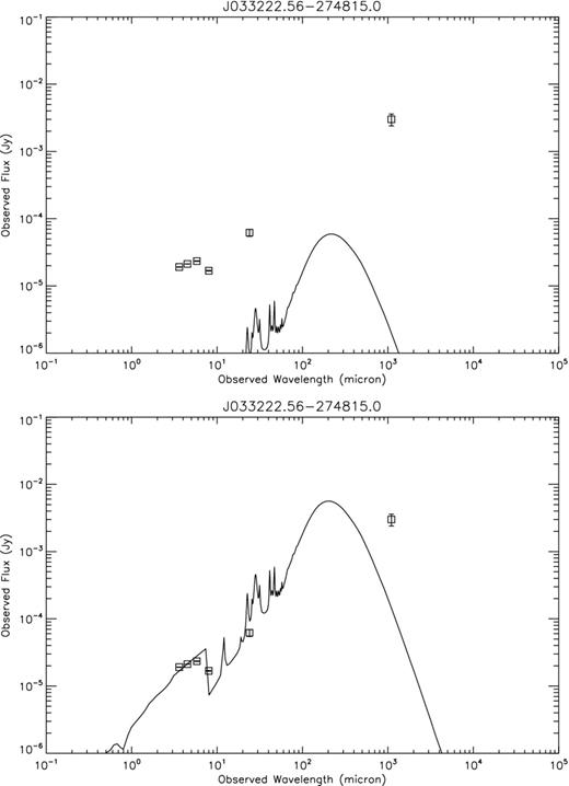
AGN only fits for J03222.56−274815.0 using the X-ray priors (top) and without (bottom). As seen in Fig. 3, the AGN component is unable to contribute any more to the NIR-to-radio SED as its vertical scaling, i.e. luminosity, is set by the X-ray priors. Without these constraints, the models are able to account for some of the mid-IR emission, still missing the bulk of the sub-mm flux, but would predict tremendous X-ray luminosities; here the best-fitting AGN L is ∼10^12.75 L_⊙, which translates to an X-ray luminosity of ∼5.9 × 10⁴⁴ erg s⁻¹, many times over what is actually observed.

Due to the underprediction of the 1.1 mm flux, we are biased to underestimate the total IR luminosity such that the values reported in Table 4 are more likely to be lower limits. Correcting for the underprediction, we can expect the luminosities to be approximately two to three times higher. As a result, the FIR-derived SFRs and the associated SFR-derived X-ray luminosities for J033215.32−275037.6 and J033207.12−275128.6 are more likely to be in line with their observed X-ray luminosities. The remaining SB-candidate X-ray sources (J033158.25−274458.8 and J100139.73+022548.5) are still ambiguous as their X-ray-derived SFRs are approximately five to eight times higher than their IR counterparts; however, the poor fits to these sources prevent an accurate measurement of their FIR luminosity and SFR, hindering our interpretation. Nevertheless, it remains plausible that at least ∼6 per cent of our X-ray-detected SMGs are SB dominated in both the IR and X-ray with little (if any) emission due to an AGN.

It is possible to account for the missing 1.1 mm flux if we relax the constraints on many of the fit parameters. For instance, the SB models can provide a better fit if we relax the redshift prior. Similarly, if the X-ray luminosity constraint is removed, then the AGN templates can account for the remaining 1.1 mm flux with significantly more dust (as set by A_V and R). These fits, however, are completely unphysical either due to inaccurate redshifts (Δz ≳ 0.5) or X-ray luminosity (unconstrained AGN templates predict orders of magnitude higher X-ray luminosities; see also Fig. 5). Instead, these additional fits suggest that an additional, possibly extended, dust distribution may be required. Similar modifications have been suggested for other SED templates in order to provide complete fits to other SMGs and millimetre-detected QSOs (e.g. Pope et al. 2008; Martínez-Sansigre et al. 2009; Rowan-Robinson et al. 2010). Unlike Rowan-Robinson et al. (2010), however, we find that a diffuse ‘cirrus’ component as described by Efstathiou & Rowan-Robinson (2003) is not sufficient for the additional dust distribution and does not improve the quality of our fits.

DISCUSSION

Across an ∼1.2 square degree area of the sky, we have analysed the X-ray spectral and NIR-to-radio SED properties of 45 X-ray-detected AzTEC sources for evidence of AGN and SB activity. Our full sample is limited by the number of available redshifts, leaving a subset (32/45) of sources. Within GOODS-N and GOODS-S, this subset of AzTEC/X-ray sources typically have high levels of dust obscuration (N_H ≳ 10²³ cm⁻²) and are generally associated with AGN activity, while their NIR-to-radio SEDs imply that the IR and bolometric output are almost completely dominated by star formation. Though we do go deeper in the 4Ms GOODS-S field and find fainter potential X-ray counterparts, we do not find any evidence for significantly higher amounts of dust obscuration compared to the 2 Ms GOODS-N and initial 2 Ms GOODS-S. Considering the relative uncertainties in the L_X–SFR relation and underprediction of the 1.1 mm flux for many of our models, a small portion (∼6–13 per cent) of our X-ray-identified SMGs are likely to be completely dominated by SB emission in both the X-ray and NIR-to-radio with the remaining majority powered almost exclusively by an AGN in the X-ray and SB in the NIR-to-radio (see Sections 3.1.3 and 3.2.2). Here, we explore the implications of our X-ray modelling and SED fitting in the context of emission at 1.1 mm and previous (sub-)mm/X-ray studies.

Origin of 1.1 mm emission

As stated in Section 3.2, (sub-)millimetre emission from our AzTEC/X-ray sources results from dust heated to T ∼ 30 K. Based on our SED fitting (Section 3.2.2), the observed NIR-to-mm luminosity is generally dominated by the SB with little contribution from an AGN (see Fig. 3). These fits predict dust temperatures of the order of ∼30–40 K yet generally underpredict the observed 1.1 mm flux by ≳50 per cent, suggesting that a cooler, extended dust component is present. Further evidence for an additional dust component has been seen in previous SMG studies (e.g. Chapman et al. 2005; Pope et al. 2006) and by Rowan-Robinson et al. (2010) in Herschel SPIRE sources, although they suggest that it can be accounted for with the cirrus templates of Efstathiou & Rowan-Robinson (2003) which we are unable verify. Fitting of the IR dust peak, for which Herschel data are optimized, will provide more accurate estimates of the dust temperature and will aid in reducing parameter uncertainty, improving the bolometric luminosity estimates and providing further insight into the nature of the missing dust.

Given the evidence so far for an additional dust component, one must wonder where the dust resides. The dust could simply reside in an extended disc if the starbursting region remains localized to the central ∼1 kpc. Alternatively, the dust may reside in the halo of the SMG, pushed out through radiation- or momentum-driven outflows resulting from the SB region(s) and/or the central AGN (e.g. Oppenheimer & Davé 2006; Zu et al. 2011). A typical GMC in a z = 2 SB galaxy can reach velocities of ∼300 km s⁻¹ (Murray, Ménard & Thompson 2011), which will spread its gas and dust as far as ∼15 kpc from the galaxy centre during an ∼50 Myr SB active phase. Similar outflows reaching ∼1000 km s⁻¹ have been observed in local ULIRGS and have been shown to account for as much as 20 per cent of the total molecular gas mass, of the order of 10⁹ M_⊙, which are easily produced through SBs with SFR ≳ 100 M_⊙ yr⁻¹ (Chung et al. 2009, 2011). The spatial scales predicted for these outflow regions are consistent with the radii predicted by the AGN templates and high-resolution imaging of SMGs using the IRAM Plateau de Bure interferometer and Submillimeter Array (e.g. Tacconi et al. 2006, 2008; Younger et al. 2008), which show typical size scales of ∼2–8 kpc. The molecular gas will not survive long due to lack of self-shielding, which would allow the dust to inhabit a larger volume than that traced by traditional molecular gas measurements. Though the majority of the mass will still be contained within the central region, the extended dust will quickly cool to the background temperature and will likely produce a temperature gradient as distance from the central region increases (see, for example, fig. 5 of Younger et al. 2008), which may contribute significantly to the (sub-)mm emission. This scenario agrees with the recent EVLA observations of Ivison et al. (2010, 2011) SMGs and of background quasars (Ménard et al. 2010).

A possible alternative to the extended cold dust model is that the missing 1.1 mm flux results from either false detections or source blending. We may readily remove false detections as the false association rate for the X-ray-identified AzTEC sources is ∼5–6 per cent (Section 2.3.1) whereas the majority of sources underpredict the 1.1 mm flux. Similarly, previous sub-mm studies suggest that blending can occur in ∼20–25 per cent of sub-mm-detected sources (see Scott et al. 2012, and references therein) so that while blending is likely to occur, it is unlikely to the primary cause for the flux discrepancy. Unfortunately, it is not possible to de-blend sources using current Spitzer MIPS, Herschel PACS or VLA radio data without a priori knowledge of the intrinsic sources. Only through high-resolution imaging and kinematics with ALMA, LMT and future (sub-)mm telescopes may we be able to de-blend potential offenders and/or make direct confirmation of an outflow-produced, extended cold dust distribution.

The question that still remains is how the AGN emission, as indicated by the high X-ray detection rate and the X-ray spectra, relates to the sub-mm observations. While AGN models are favoured in the X-ray spectral fitting, the sub-mm emission is, in fact, unlikely to result solely from an AGN. As shown in Fig. 5, the X-ray priors prevent any significant contribution from the AGN templates. Even when relaxed, the AGN models still show poor fits to the mid-IR, relative to their observed fluxes and uncertainties, and sub-mm data, irrespective of the unphysical X-ray luminosity predicted. In a merger-driven formation scenario (e.g. Narayanan et al. 2010), gas from the colliding systems gives rise to an increase in star formation, resulting in a sub-mm-bright phase. Shortly after the sub-mm-bright phase and final coalescence, the central black hole may undergo the bulk of its growth, producing an AGN which may then aid in shutting off the star formation through feedback, leaving the final system as a quasar or dusty AGN-powered ULIRG. Given the high X-ray column densities we derived for our AzTEC/X-ray sample, it is likely that these sources represent the early growth phase of the AGN. Combined with the SB-dominated NIR-to-radio SEDs and expected short time-scale of the sub-mm-bright phase (<50 Myr), the X-ray-identified sources may be SMGs caught in their transitionary period between peak star formation and peak black hole growth. This transition scenario is consistent with the fact that the average 1.1 mm fluxes and 2–10 keV count rates of the X-ray-identified sources are both below the average of the overall SMG and X-ray sample. The remaining X-ray-undetected SMGs could result from an SB triggered during the first passing of merging systems or rapid, short-lived mergers similar to those found by Chapman et al. (2009). However, we cannot rule out the possibility that the X-ray-dim SMGs could result from a moderately continuous gas in-fall (see, for example, Davé et al. 2010) or very young SBs with Compton-thick AGNs (e.g. A05a,b). The X-ray-detected SMGs are unlikely to be produced by such continuous in-fall given the SB time-scales from our SED modelling; accretion-driven models predict that the sub-mm-bright phase may last for ∼0.1–1 Gyr (Fardal et al. 2001). One other possibility given the expected high SFRs for SMGs is that the central AGNs are likely time-variable (see Alexander & Hickox 2012, and references therein). AGN can switch between being ‘on’ or ‘off’ on time-scales of ≲1 yr and cause large variations in their observed luminosities and absorbing column densities, which will affect the probability of detecting an AGN associated with an SMG. It is unknown how this AGN time-variability scenario will influence the SED of SMGs though we expect any contribution to be small given the already low AGN contribution rate. Further evolutionary simulations and observations aimed at spatially resolving SMGs will provide the tools necessary to classify SMGs under the appropriate formation and evolutionary scenario.

Comparison with previous studies

For our AzTEC/X-ray sample, the AGN detection rate is ∼14 per cent between all three fields. However, the shallow X-ray depth of COSMOS, potentially compounded by our more stringent detection criteria, prevents confirmation of the most heavily obscured AGNs which may contribute significantly to the sub-mm emission (Lutz et al. 2010; Hill & Shanks 2011). Excluding COSMOS, the AGN detection rate increases to ∼28 per cent, consistent with previous X-ray/SMG studies ( > 38|$ {^{+ 12}_{-10}} $|⁠, 29 ± 8 and <26 ± 9 per cent for A05a,b, LNPS10 and GRC11, respectively) while avoiding potential biases due to prior counterpart identification and achieving better source statistics via larger sky coverage. Similar to LNPS10, we also find evidence that ∼6–13 per cent of our X-ray sources are potentially HMXBs associated with high SFRs. However, many of the SB-powered SCUBA-detected sources of LNPS10, and by extension A05b, are missing from our sample. While our X-ray data for GOODS-N are essentially the same as those used in A05b and LNPS10, it is not surprising for differences to exist between the AzTEC and SCUBA catalogues. Chapin et al. (2009) suggest that such a discrepancy results from instrument and measurement calibration uncertainty as well as intrinsic spread in host properties (namely dust temperature and emissivity). In fact, for a SCUBA source to be detected by AzTEC at >3.5σ in GOODS-N (where the AzTEC rms is ∼1.3 mJy beam⁻¹; see Section 2.1), its effective 850 μm flux would need to be ≳8.19 mJy, higher than the typical 850 μm flux for sources in LNPS10. This estimate assumes an R = S₈₅₀/S_1.1 value of 1.8 (Chapin et al. 2009) and that ‘flux boosting’ (see, for example, Austermann et al. 2010; Scott et al. 2010) affects the 850 μm and 1.1 mm observations equally. Completeness of the (sub-)mm observations may also contribute to this discrepancy; at ∼4 mJy, the AzTEC map is ∼60 per cent complete (Perera et al. 2008). Of course, there is always the issue of false identifications and mismatching of sources as well as prior counterpart bias (see LNPS10) which, while the expected number of such occurrences is small (see Section 2), may still lead to a decrease in the number of SB-dominated X-ray sources in our sample.

In Fig. 6, we show the range of effective photon indices Γ_Eff for our AzTEC/X-ray sample (see Section 3.1.1, Table 3) in relation to the samples of A05b and LNPS10. Using the Mann–Whitney (MW) U-test, we find that the probability that our AzTEC/X-ray sources are consistent with being drawn from the samples of A05b and LNPS10 is 0.02 and 0.14, respectively. If we limit our sample to AzTEC/X-ray sources with radio detections, then the MW probabilities become 0.07 and 0.17 for the A05b and LNPS10 samples, respectively. Since the errors on Γ_Eff are known, we further estimate the intrinsic mean and variance of the samples by constructing 1000 Monte Carlo realizations of the Γ_Eff distributions. The resulting intrinsic mean values of Γ_Eff for the AzTEC/X-ray, A05b and LNPS10 samples are 1.14 ± 0.09 (1σ), 0.60 ± 0.10 and 1.44 ± 0.16, respectively; including only the radio-detected AzTEC/X-ray sources results in an intrinsic mean of 1.05 ± 0.08. These results imply a strong statistical difference between the AzTEC/X-ray and A05b samples (at ≳3σ), while the AzTEC/X-ray and LNPS10 samples have consistent mean values of Γ_Eff.

Figure 6.

Open in new tab Download slide

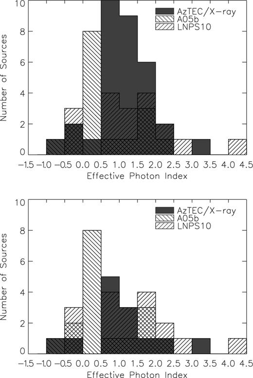
Histogram of effective power-law indices (Γ_Eff) for the AzTEC/X-ray sources, given by the filled histogram, for all sources (top) and only those with radio counterparts (bottom). For comparison, we also include the Γ_Eff distributions from A05b (back-hashed region) and LNPS10 (forward-hashed region).

Despite the differences in Γ_Eff, the methods of analysis in A05b produce results consistent with our study. For further comparison, we reproduce figs 2b and 8 of A05b, which show the |$L_{{\rm 2.0{\rm -}10.0\, keV}}$| versus L_1.4 GHz (Fig. 7) and |$L_{{\rm 2.0{\rm -}10.0 keV}}$| versus L_FIR (Fig. 8) relations for the A05b and LNPS10 SB and AGN systems, including our AzTEC/X-ray sources that have radio counterparts. In reproducing the A05b figures, we have converted the A05b 0.5–8.0 keV fluxes to 2.0–10.0 keV luminosities assuming a photon index of Γ = 1.8 and equation 1 of Alexander et al. (2003). Radio and FIR luminosities have been determined for our sample following the same procedures as in A05b to ensure compatibility. We caution, however, that the radio–FIR correlation used to derive the FIR luminosities from the radio emission (Helou et al. 1985) assumes emission purely from star formation and could be misleading if the AGN is radio-loud (e.g. Donley et al. 2005, 2010). Figs 7 and 8 show that the X-ray emission for the subsample of radio-identified AzTEC/X-ray sources is higher than one would predict from their radio and/or FIR luminosities if they resulted purely from star formation, indicating AGN activity. However, the FIR luminosities are generally higher than expected for typical quasars which suggests significant contribution from star formation, again consistent with the results from Section 3.2. Alternatively, sources could lie above the Elvis et al. (1994) quasar relation if they are reflection dominated or Compton-thick (e.g. FSC 10214+4727, A05b; Arp 220, Iwasawa et al. 2005). This is not likely to affect our analysis based on the results from our X-ray spectral modelling (Section 3.1); nevertheless, we cannot rule out the possibility that the faintest X-ray sources may be harbouring highly luminous, Compton-thick AGNs, particularly for the non-X-ray-detected SMGs (e.g. Iwasawa et al. 2005; Lutz et al. 2010; Hill & Shanks 2011).

Figure 7.

Open in new tab Download slide

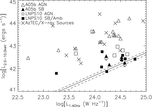
Reproduction of fig. 2b from A05b including the A05b, LNPS10 and AzTEC/X-ray samples. The fluxes of A05b have been converted to 2.0–10.0 keV luminosities assuming a photon index of Γ = 1.8 and equation 1 of Alexander et al. (2003). Radio luminosities are calculated from the radio fluxes in Table 2 and equation 2 of Alexander et al. (2003). Also plotted is the P04 SFR–X-ray luminosity relation (solid line), using the SFR–radio relation of Condon (1992) to convert SFR to 1.4 GHz luminosity, with a 20 per cent statistical error given by the dotted lines. Some of the A05b SB sources only have 3σ upper limits for their X-ray luminosities and are shown with arrows as indicated.

Figure 8.

$Reproduction of fig. 8 from A05b including the A05b, LNPS10 and AzTEC/X-ray samples. The X-ray fluxes of A05b are converted to 2.0–10.0 keV using Γ = 1.8. FIR luminosities are derived from the radio luminosities of Fig. 7 using a radio to FIR correlation of q = 2.35 (Helou, Soifer & Rowan-Robinson 1985). The overplotted lines represent ratios of constant X-ray versus FIR luminosity for the A05b SB ($\frac{L_{\rm X}}{L_{\rm {FIR}}} = 10^{-4}$) and AGN ($\frac{L_{\rm X}}{L_{{\rm FIR}}}$ = 0.004) sources, and the average luminosity ratio for quasars studied by Elvis et al. (1994) ($\frac{L_{\rm X}}{L_{{\rm FIR}}}$ = 0.05).$

Open in new tab Download slide

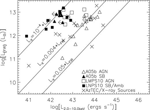
Reproduction of fig. 8 from A05b including the A05b, LNPS10 and AzTEC/X-ray samples. The X-ray fluxes of A05b are converted to 2.0–10.0 keV using Γ = 1.8. FIR luminosities are derived from the radio luminosities of Fig. 7 using a radio to FIR correlation of q = 2.35 (Helou, Soifer & Rowan-Robinson 1985). The overplotted lines represent ratios of constant X-ray versus FIR luminosity for the A05b SB (⁠|$\frac{L_{\rm X}}{L_{\rm {FIR}}} = 10^{-4}$|⁠) and AGN (⁠|$\frac{L_{\rm X}}{L_{{\rm FIR}}}$| = 0.004) sources, and the average luminosity ratio for quasars studied by Elvis et al. (1994) (⁠|$\frac{L_{\rm X}}{L_{{\rm FIR}}}$| = 0.05).

Cross-correlation of AzTEC/X-ray source populations

In addition to examining X-ray-detected SMGs on a source-by-source basis, a simple cross-correlation analysis of the X-ray and AzTEC source populations can identify evolutionary patterns between the populations. Almaini (2002) and Almaini et al. (2003) were the first to measure the angular cross-correlation function (XCF) between SMGs and X-ray sources and found significant correlation at large scales, leading to the conclusion that the populations both reside in similarly massive dark matter haloes and trace the same large-scale structure. Hill & Shanks (2011) later estimated the XCF for LABOCA sources in the ECDFS, and found similar evidence for small-scale clustering, i.e. residing in same dark matter haloes, but no evidence for large-scale clustering, consistent with Borys et al. (2004). Roche, Dunlop & Almaini (2003) measured the XCF of extremely red objects (EROs) – which may be the signature of massive galaxies that have entered their passive post-AGN phase in galaxy evolution – and X-ray sources in the CDFS, and again find evidence for significant correlation. Together, these results may suggest an evolutionary sequence between these three populations, where SB-dominated SMGs go through an AGN-bright phase before evolving into passive ellipticals or EROs.

To determine if there is any correlation between the AzTEC and Chandra source populations, we apply the two-point angular XCF, w_AX(θ), defined as the excess probability of finding both an AzTEC source in a solid angle δΩ_A and an X-ray source in a solid angle δΩ_X, with an angular separation θ from each other. This excess probability (relative to an uncorrelated distribution) is given by δP = ρ_Aρ_X[1 + w_AX(θ)]δΩ_AδΩ_X, where ρ_A and ρ_X are the surface densities of AzTEC and X-ray galaxies on the sky (Peebles 1980). In practice, this can be measured from galaxy maps by counting the number of SMG/X-ray source pairs, binned by their angular separation, and comparing to pair counts from random positions. Here, we use the cross-correlation adaptation to the Landy–Szalay estimator (Landy & Szalay 1993), which is given by

\begin{equation} w_{AX}(\theta ) = \frac{D_{A}D_{X}(\theta )-D_{A}R_{X}(\theta )-D_{X}R_{A} (\theta )+R_{A}R_{X}(\theta )}{R_{A}R_{X}(\theta )}, \end{equation}

(3)

where D_AD_X is the number of SMG/X-ray source pairs, D_AR_X and D_XR_A are the number of pairs found between each galaxy catalogue and randomly generated positions of sources within each angular separation bin. R_AR_X is the number of pairs found between random positions for each galaxy population, generated from the selection function and sensitivity distribution of each map. To generate random source distributions for the AzTEC maps, we follow the methods of Williams et al. (2011). For the Chandra random catalogues, the exposure maps are relatively uniform (ignoring effects due to CCD gaps and edge overlapping in COSMOS as they are generally small) such that we may produce the random catalogues by simply randomly generating positions within the overlapping coverage region of the Chandra and AzTEC maps. Note, however, that this does not take into account the sensitivity variations (mostly due to PSF degradation) as a function of off-axis distance; the XCF may thus be incorrect at scales larger than ∼200 arcsec. The overlapping observations in COSMOS help to smooth the telescope response, allowing for a more accurate XCF at larger scales.

The resulting XCF for each field, as well as the expected XCF from completely random distributions, is shown in Fig. 9, where the errors are estimated from a Poissonian distribution given the number of AzTEC/X-ray pairs in each angular bin. The expectation from random distributions is estimated by averaging the XCF of 100 AzTEC and X-ray random distributions described above, which have the same properties (area and source density) as the observed maps. In the case of the random expectation, the errors correspond to the standard deviation of the XCF from each of the individual random distributions. At small scales, there is significant positive correlation in the observed XCF due to identified counterparts (see also Hill & Shanks 2011); this effect is diluted in COSMOS due to its shallow X-ray depth and thus low source density compared to either GOODS field. However, since the AzTEC source positions are not well known on scales smaller than the beam size, we choose to limit our XCF analysis to the large-scale clustering. Fig. 10 shows the same XCF combined with their weighted average for scales larger than 28 arcsec, the beam size of AzTEC on ASTE, though we caution against heavy interpretation at scales larger than ∼200 arcsec as previously mentioned.

Figure 9.

Open in new tab Download slide

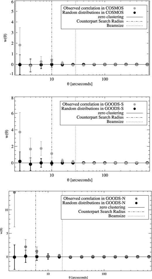
The XCF between AzTEC and Chandra source populations. Plotted in each panel is the observed XCF and the XCF from randomly generated source populations along with the respective beam size and search radius for each field. Below our adopted search radii, the XCF shows significant signal due to detected counterparts. The lack of consistent positive correlation in COSMOS results from the shallow X-ray depth and corresponding low source density.

Figure 10.

Open in new tab Download slide

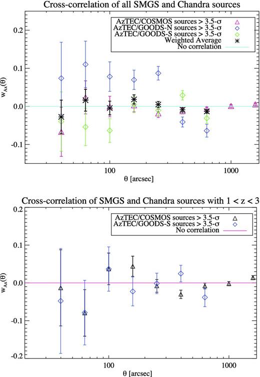
The XCF between the AzTEC and Chandra source populations (shown in Fig. 9) at scales larger than the beam size. The top panel shows the full sample, while the bottom shows the XCF in the redshift range 1<z <3. Over the three fields, there is no significant correlation between the source populations, particularly over the typical redshift range of SMGs. Due to sensitivity variations in the Chandra data, the XCF should not be heavily weighed at angular separations of ≳200.

Across the three fields, we find no evidence for any large-scale correlation signal; any apparent correlation or anticorrelation seen in individual fields is detected at ≲1σ confidence, consistent with Borys et al. (2004) and Hill & Shanks (2011). The large area covered by our sample (∼1.2 square degrees) aids in mitigating the effects of cosmic variance, which is the likely cause of variation between fields and may affect the positive correlation signal found in Almaini (2002). It is possible that the lack of any correlation signal in our data may be the result of dilution given the wide and differing redshift distributions of the X-ray and sub-mm sources. In an attempt to improve the cross-correlation signal, we have run the same analysis by limiting the X-ray sources to the redshift range 1 < z < 3 where the X-ray redshift distribution shows significant overlap with the sub-mm distribution. If there is any cross-correlation between the two samples, it should be maximized here. Due to the small number of X-ray sources with available redshifts in GOODS-N (49 out of the original 397), we excluded this field from the XCF in the 1<z <3 redshift range. The XCF using this redshift-limited subset for GOODS-S and COSMOS is statistically identical to the result we measured using the entire set of X-ray sources, i.e. no evidence for a correlation.

The lack of a significant correlation between the X-ray and AzTEC source populations at large scales may suggest that SMGs and AGN are not universally related in terms of dark matter halo mass and large-scale structure. However, considering the significant fraction of AzTEC SMGs that do have plausible X-ray detections here, it is likely that the SMG phenomenon is not governed by a single formation and evolution process; rather, the SMG population is a ‘mixed bag’ of systems – some undergoing major mergers concurrent with the build-up of massive black holes (e.g. Narayanan et al. 2010) and others signalling a short-lived phase of intense star formation in more normal galaxies (e.g. Chapman et al. 2009) or even quiescent mass build-up from gas in-fall (e.g. Davé et al. 2010) (see also Section 4.1). Such cases are likely tied to the host's intrinsic properties which could naturally explain the enhanced sub-mm emission from bright, obscured AGNs as found by Lutz et al. (2010) and Hill & Shanks (2011). However, we caution that limitations in measuring the correlation between these populations can also give a null result. For example, the large-volume sample coupled with the lack of redshift information for the full X-ray and SMG catalogues will necessarily dilute the projected correlation strength between the two populations, even if there is some spatial correlation. The shallow X-ray depth of COSMOS will further dilute any correlation signal by primarily detecting bright AGN that are likely well past their SB phase. Observations of SMGs in the near future with ALMA and the LMT geared towards measuring their redshifts and obtaining high-resolution imaging of their dust and gas will greatly aid in the development and fine tuning of formation and evolution scenarios for this population.

SUMMARY

We have presented a detailed analysis of the X-ray properties of AzTEC 1.1 mm sources found in the GOODS-N, GOODS-S and COSMOS fields. Thanks to deep (∼2–4 Ms) Chandra observations, we find X-ray counterparts to ∼14 per cent of the 1.1 mm sources across all three fields, increasing to ∼28 per cent if we exclude COSMOS due to its shallower X-ray data. From our modelling of the X-ray spectra and NIR-to-radio SEDs, we conclude that AzTEC/X-ray sources are all SB dominated in the IR, with SFRs of the order of 100–1000 M_⊙ yr⁻¹, whereas an AGN component is needed in order to explain the observed X-ray luminosities for the majority of our sources. In ∼6–13 per cent of our sample, we find evidence for X-ray emission consistent with high SFRs, after accounting for the relative uncertainties in the L_X–SFR relations and the typical underprediction of the 1.1 mm flux in our SED modelling. The AGNs typically appear obscured in the X-ray band, with neutral hydrogen column densities in excess of 10²³ cm⁻². These results are consistent with other SMG/X-ray studies. Overall, the AGN templates contribute very little (≲10 per cent) to both the bolometric luminosity and 1.1 mm flux. At 1.1 mm in particular, the AGN+SB models typically underpredict the observed fluxes, which indicates that either a cooler, extended dust component is required to fully recover the NIR-to-radio SED or the sources are blended. We suggest that this missing dust could result from radiation- and/or momentum-driven outflows caused by the SB/AGN regions, which pushes the dust out into the halo where it cools rapidly and, although it accounts for a small fraction of the total dust mass, may contribute significantly to the 1.1 mm emission.

The high AGN identification rate in these AzTEC SMGs is particularly interesting in regard to SMG formation and evolution scenarios. Following a merger-driven scenario, the X-ray-identified sources could represent the transitional period between SB and AGN dominant phases. However, the lack of a significant correlation at large scales between all X-ray sources and SMGs in these fields suggests that not all SMGs will evolve to possess an AGN and, similarly, that not all AGN evolve from a sub-mm-bright phase. This suggests heterogeneity in the formation/evolution of SMGs, possibly due to either intrinsic source properties, i.e. amount of obscuration, or even multiple formation scenarios. With future analyses aimed at source evolution as a function of redshift, combined with a more comprehensive redshift catalogue for SMGs (one of the goals for the upcoming LMT), we will be able to determine the AGN fraction and contribution to greater certainty, allowing for investigating how SMGs form and evolve into the galaxies we see in the local Universe.

We would like to thank the AzTEC team, M. Giavalisco, M. Lacy and the anonymous reviewer for discussions and helpful comments in developing this manuscript. This work has been funded under NSF grants AST-0907952 and AST-0838222, and CXC grant SAO SP1-12003X. MK was supported in part by Mid-career Researcher Programme through the National Research Foundation of Korea (NRF) funded by the Ministry of Education, Science and Technology 2011-0028001. KSS is supported by the National Radio Astronomy Observatory, which is a facility of the National Science Foundation operated under cooperative agreement by Associated Universities, Inc.

1

http://www.astro.yale.edu/dokkum/simple/

2

http://www.stsci.edu/science/goods/

3

http://ssc.spitzer.caltech.edu/legacy/abs/dickinson2.html

4

http://irsa.ipac.caltech.edu/Missions/cosmos.html

REFERENCES

Alexander

D. M.

,

Hickox

R. C.

. ,

New Astron. Rev.

,

2012

, vol.

46

pg.

93

Crossref

Search ADS

Alexander

D. M.

, et al. ,

AJ

,

2003

, vol.

126

pg.

539

Crossref

Search ADS

Alexander

D. M.

,

Smail

I.

,

Bauer

F. E.

,

Chapman

S. C.

,

Blain

A. W.

,

Brandt

W. N.

,

Ivison

R. J.

. ,

Nat

,

2005a

, vol.

434

pg.

738

A05a

Crossref

Search ADS

Alexander

D. M.

,

Bauer

F. E.

,

Chapman

S. C.

,

Smail

I.

,

Blain

A. W.

,

Brandt

W. N.

,

Ivison

R. J.

. ,

ApJ

,

2005b

, vol.

632

pg.

736

A05b

Crossref

Search ADS

Almaini

O.

.

Metcalfe

N.

,

Shanks

T.

. ,

ASP Conf. Ser. Vol. 283, A New Era in Cosmology

,

2002

San Francisco

Astron. Soc. Pac.

pg.

377

Google Scholar

Google Preview

OpenURL Placeholder Text

WorldCat

Almaini

O.

, et al. ,

MNRAS

,

2003

, vol.

338

pg.

303A

Crossref

Search ADS

Aretxaga

I.

, et al. ,

MNRAS

,

2011

, vol.

415

pg.

3831

Crossref

Search ADS

Arnaud

K. A.

.

Jacoby

G.

,

Barnes

J.

. ,

ASP Conf. Ser. Vol. 101, Astronomical Data Analysis Software and Systems V

,

1996

San Francisco

Astron. Soc. Pac.

pg.

17

Google Scholar

Google Preview

OpenURL Placeholder Text

WorldCat

Austermann

J. E.

, et al. ,

MNRAS

,

2010

, vol.

401

pg.

160

Crossref

Search ADS

Barger

A. J.

, et al. ,

AJ

,

2003

, vol.

126

pg.

632

Crossref

Search ADS

Barger

A. J.

,

Cowie

L. L.

,

Wang

W.-H.

. ,

ApJ

,

2008

, vol.

689

pg.

687

Crossref

Search ADS

Bertoldi

F.

, et al. ,

ApJS

,

2007

, vol.

172

pg.

132

Crossref

Search ADS

Bielby

R. M.

,

Hill

M. D.

,

Metcalfe

N.

,

Shanks

T.

. ,

MNRAS

,

2012

, vol.

419

pg.

1315

Crossref

Search ADS

Blain

A. W.

,

Smail

I.

,

Ivison

R. J.

,

Kneib

J.-P.

,

Frayer

D. T.

. ,

Phys. Rep.

,

2002

, vol.

369

pg.

111

Crossref

Search ADS

Blain

A. W.

,

Chapman

S. C.

,

Smail

I.

,

Ivison

R.

. ,

ApJ

,

2004

, vol.

611

pg.

52

Crossref

Search ADS

Borys

C.

,

Scott

D.

,

Chapman

S.

,

Halpern

M.

,

Nandra

K.

,

Pope

A.

. ,

MNRAS

,

2004

, vol.

355

pg.

485

Crossref

Search ADS

Carilli

C. L.

,

Yun

M. S.

. ,

ApJ

,

2000

, vol.

530

pg.

618

Crossref

Search ADS

Cash

W.

. ,

ApJ

,

1979

, vol.

228

pg.

939

Crossref

Search ADS

Chapin

E. L.

, et al. ,

MNRAS

,

2009

, vol.

398

pg.

1793

Crossref

Search ADS

Chapman

S. C.

,

Blain

A. W.

,

Smail

I.

,

Ivison

R. J.

. ,

ApJ

,

2005

, vol.

622

pg.

772

Crossref

Search ADS

Chapman

S. C.

,

Blain

A. W.

,

Ibata

R.

,

Ivison

R. J.

,

Smail

I.

,

Morrison

G.

. ,

ApJ

,

2009

, vol.

691

pg.

560

Crossref

Search ADS

Chung

A.

,

Narayanan

G.

,

Yun

M. S.

,

Heyer

M.

,

Erickson

N. R.

. ,

ApJ

,

2009

, vol.

138

pg.

858

Crossref

Search ADS

Chung

A.

,

Yun

M. S.

,

Narayanan

G.

,

Heyer

M.

,

Erickson

N. R.

. ,

ApJ

,

2011

, vol.

732

pg.

15

Crossref

Search ADS

Condon

J. J.

. ,

ARA&A

,

1992

, vol.

30

pg.

575

Crossref

Search ADS

Coppin

K. E.

, et al. ,

MNRAS

,

2006

, vol.

372

pg.

1621

Crossref

Search ADS

Coppin

K. E.

, et al. ,

MNRAS

,

2008

, vol.

389

pg.

45

Crossref

Search ADS

Davé

R.

,

Finlator

K.

,

Oppenheimer

B. D.

,

Fardal

M.

,

Katz

N.

,

Keres

D.

,

Weinberg

D. H.

. ,

MNRAS

,

2010

, vol.

404

pg.

1355

de Zotti

G.

,

Massardi

M.

,

Negrello

M.

,

Wall

J.

. ,

A&AR

,

2010

, vol.

18

pg.

1

Crossref

Search ADS

Dicken

D.

, et al. ,

ApJ

,

2012

, vol.

745

pg.

172

Crossref

Search ADS

Donley

J. L.

,

Rieke

G. H.

,

Rigby

J. R.

,

Pérez-González

P. G.

. ,

ApJ

,

2005

, vol.

634

pg.

169

Crossref

Search ADS

Donley

J. L.

,

Rieke

G. H.

,

Alexander

D. M.

,

Egami

E.

,

Pérez-González

P. G.

. ,

ApJ

,

2010

, vol.

719

pg.

1393

Crossref

Search ADS

Downes

A. J.

,

Peacock

J. A.

,

Savage

A.

,

Carrie

D. R.

. ,

MNRAS

,

1986

, vol.

218

pg.

31

Crossref

Search ADS

Downes

T. P.

,

Welch

D.

,

Scott

K. S.

,

Austermann

J.

,

Wilson

G. W.

,

Yun

M. S.

. ,

MNRAS

,

2012

, vol.

423

pg.

529

Crossref

Search ADS

Efstathiou

A.

,

Rowan-Robinson

M.

. ,

MNRAS

,

2003

, vol.

343

pg.

322

Crossref

Search ADS

Efstathiou

A.

,

Rowan-Robinson

M.

,

Siebenmorgen

R.

. ,

MNRAS

,

2000

, vol.

313

pg.

734

Crossref

Search ADS

Elvis

M.

, et al. ,

ApJS

,

1994

, vol.

95

pg.

1

Crossref

Search ADS

Elvis

M.

, et al. ,

ApJS

,

2009

, vol.

184

pg.

158

Crossref

Search ADS

Fardal

M.

,

Katz

N.

,

Weinberg

D. H.

,

Davé

R.

,

Hernquist

L.

. ,

ApJ

,

2001

preprint (astro-ph/0107290v1)

Ferrarese

F.

,

Merritt

D.

. ,

ApJ

,

2000

, vol.

539

pg.

9

Crossref

Search ADS

Fritz

J.

,

Franceshini

A.

,

Hatziminaoglou

E.

. ,

MNRAS

,

2006

, vol.

266

pg.

767

Crossref

Search ADS

Gebhardt

K.

, et al. ,

ApJ

,

2000

, vol.

539

pg.

13

Crossref

Search ADS

Georgantopoulos

I.

,

Rovilos

E.

,

Comastri

A.

. ,

A&A

,

2011

, vol.

526

pg.

A46

GRC11

Crossref

Search ADS

Granato

G. L.

,

Danese

L.

. ,

MNRAS

,

1994

, vol.

268

pg.

235

Crossref

Search ADS

Gultekin

, et al. ,

ApJ

,

2009

, vol.

698

pg.

198

Crossref

Search ADS

Helou

G.

,

Soifer

B. T.

,

Rowan-Robinson

M.

. ,

ApJ

,

1985

, vol.

298

pg.

7

Crossref

Search ADS

Heywood

I.

,

Bielby

R. M.

,

Hill

M. D.

,

Metcalfe

N.

,

Rawlings

S.

,

Shanks

T.

,

Smirnov

O. M.

. ,

MNRAS

,

2012

, vol.

410

pg.

762

Hill

M. D.

,

Shanks

T.

. ,

MNRAS

,

2011

, vol.

410

pg.

762

Crossref

Search ADS

Holland

W. S.

, et al. ,

MNRAS

,

1999

, vol.

303

pg.

659

Crossref

Search ADS

Hopkins

P. F.

,

Younger

J. D.

,

Hayward

C. C.

,

Narayanan

D.

,

Hernquist

L.

. ,

MNRAS

,

2010

, vol.

402

pg.

1693

Crossref

Search ADS

Hughes

D. H.

, et al. ,

Nat

,

1998

, vol.

394

pg.

241

Crossref

Search ADS

Ivison

R. J.

, et al. ,

MNRAS

,

2007

, vol.

380

pg.

199

Crossref

Search ADS

Ivison

R. J.

,

Smail

I.

,

Papadopoulos

P. P.

,

Wold

I.

,

Richard

J.

,

Swinbank

A. M.

,

Kneib

J.-P.

,

Owen

F. N.

. ,

MNRAS

,

2010

, vol.

404

pg.

198

Ivison

R. J.

,

Papadopoulos

P. P.

,

Smail

I.

,

Greve

T. R.

,

Thomson

A. P.

,

Xilouris

E. M.

,

Chapman

S. C.

. ,

MNRAS

,

2011

, vol.

412

pg.

1913

Crossref

Search ADS

Iwasawa

K.

,

Sanders

D. B.

,

Evans

A. S.

,

Trentham

N.

,

Miniutti

G.

,

Spoon

H. W. W.

. ,

MNRAS

,

2005

, vol.

357

pg.

565

Crossref

Search ADS

Kellermann

K. I.

,

Fomalont

E. B.

,

Mainieri

V.

,

Padovani

P.

,

Rosati

P.

,

Shaver

P.

,

Tozzi

P.

,

Miller

N.

. ,

ApJS

,

2008

, vol.

179

pg.

71

Crossref

Search ADS

Kennicutt

R. C.

. ,

ARA&A

,

1998

, vol.

36

pg.

189

Crossref

Search ADS

Laird

E. S.

,

Nandra

K.

,

Pope

A.

,

Scott

D.

. ,

MNRAS

,

2010

, vol.

401

pg.

2763

LNPS10

Crossref

Search ADS

Landy

S. D.

,

Szalay

A. S.

. ,

ApJ

,

1993

, vol.

412

pg.

64

Crossref

Search ADS

Le Floc'h

E.

, et al. ,

ApJ

,

2005

, vol.

632

pg.

169

Crossref

Search ADS

Lucy

L. B.

. ,

MNRAS

,

2000

, vol.

318

pg.

92

Crossref

Search ADS

Luo

B.

, et al. ,

ApJS

,

2008

, vol.

179

pg.

19

Crossref

Search ADS

Lutz

D.

, et al. ,

ApJ

,

2010

, vol.

712

pg.

1287

Crossref

Search ADS

Marconi

A.

,

Risaliti

G.

,

Gilli

R.

,

Hunt

L. K.

,

Maiolino

R.

,

Salvati

M.

. ,

MNRAS

,

2004

, vol.

351

pg.

169

Crossref

Search ADS

Martínez-Sansigre

A.

, et al. ,

ApJ

,

2009

, vol.

706

pg.

184

Crossref

Search ADS

Ménard

B.

,

Scranton

R.

,

Fukugita

M.

,

Richards

G.

. ,

MNRAS

,

2010

, vol.

405

pg.

1025

Menéndez-Delmestre

K.

, et al. ,

ApJ

,

2007

, vol.

655

pg.

65

Crossref

Search ADS

Menéndez-Delmestre

K.

, et al. ,

ApJ

,

2009

, vol.

699

pg.

667

Crossref

Search ADS

Meng

X.-M.

,

Wu

H.

,

Gu

Q.-S.

,

Wang

J.

,

Cao

C.

. ,

ApJ

,

2010

, vol.

718

pg.

928

Crossref

Search ADS

Merloni

A.

. ,

MNRAS

,

2004

, vol.

353

pg.

1035

Crossref

Search ADS

Miller

N. A.

,

Fomalont

E. B.

,

Kellermann

K. I.

,

Mainieri

V.

,

Norman

C.

,

Padovani

P.

,

Rosati

P.

,

Tozzi

P.

. ,

ApJS

,

2008

, vol.

179

pg.

114

Crossref

Search ADS

Mineo

S.

,

Gilfanov

M.

,

Sunyaev

R.

. ,

MNRAS

,

2012

, vol.

419

pg.

2095

Crossref

Search ADS

Morrison

G. E.

,

Owen

F. N.

,

Dickinson

M.

,

Ivison

R. J.

,

Ibar

E.

. ,

ApJS

,

2010

, vol.

188

pg.

178

Crossref

Search ADS

Murray

N.

,

Ménard

B.

,

Thompson

T. A.

. ,

ApJ

,

2011

, vol.

735

pg.

66

Crossref

Search ADS

Nandra

K.

,

Pounds

K.

. ,

MNRAS

,

1994

, vol.

268

pg.

405

Crossref

Search ADS

Narayanan

D.

,

Hayward

C. C.

,

Cox

T. J.

,

Hernquist

L.

,

Jonsson

P.

,

Younger

J. D.

,

Groves

B.

. ,

MNRAS

,

2010

, vol.

401

pg.

1613

Crossref

Search ADS

Nardini

E.

,

Risaliti

G.

,

Salvati

M.

,

Sani

E.

,

Imanishi

M.

,

Marconi

A.

,

Maiolino

R.

. ,

MNRAS

,

2008

, vol.

385

pg.

130

Crossref

Search ADS

Nenkova

M.

,

Sirocky

M. M.

,

Ivezic

Z.

,

Elitzur

M.

. ,

ApJ

,

2008

, vol.

685

pg.

147

Crossref

Search ADS

Oppenheimer

B. D.

,

Davé

R.

. ,

MNRAS

,

2006

, vol.

373

pg.

1265

Crossref

Search ADS

Peebles

P. J. E.

. ,

The Large Scale Structure of the Universe

,

1980

Princeton, NJ

Princeton Univ. Press

Google Scholar

Google Preview

OpenURL Placeholder Text

WorldCat

Perera

T. A.

, et al. ,

MNRAS

,

2008

, vol.

391

pg.

1227

Crossref

Search ADS

Pérez-González

P. G.

, et al. ,

ApJ

,

2005

, vol.

630

pg.

82

Crossref

Search ADS

Persic

M.

,

Rephaeli

Y.

. ,

A&A

,

2002

, vol.

382

pg.

843

Crossref

Search ADS

Persic

M.

,

Rephaeli

Y.

. ,

A&A

,

2007

, vol.

463

pg.

481

Crossref

Search ADS

Persic

M.

,

Rephaeli

Y.

,

Braito

V.

,

Cappi

M.

,

Della Ceca

R.

,

Franceschini

A.

,

Gruber

D. E.

. ,

A&A

,

2004

, vol.

419

pg.

849

P04

Crossref

Search ADS

Pope

A.

, et al. ,

MNRAS

,

2006

, vol.

370

pg.

1185

Crossref

Search ADS

Pope

A.

, et al. ,

ApJ

,

2008

, vol.

675

pg.

1171

Crossref

Search ADS

Ranalli

P.

,

Comastri

A.

,

Setti

G.

. ,

A&A

,

2003

, vol.

399

pg.

39

Crossref

Search ADS

Roche

N. D.

,

Dunlop

J.

,

Almaini

O.

. ,

MNRAS

,

2003

, vol.

346

pg.

803

Crossref

Search ADS

Rowan-Robinson

M.

, et al. ,

MNRAS

,

2010

, vol.

409

pg.

2

Crossref

Search ADS

Santini

P.

, et al. ,

A&A

,

2009

, vol.

504

pg.

751

Crossref

Search ADS

Schloerb

F. P.

. ,

Proc. SPIE, ed. Stepp L. M., Gilmozzi R.

,

2008

, vol.

7012E

pg.

26

Scott

K. S.

, et al. ,

MNRAS

,

2010

, vol.

405

pg.

2260

Scott

K. S.

, et al. ,

MNRAS

,

2012

, vol.

423

pg.

575

Crossref

Search ADS

Sejeant

S.

, et al. ,

A&A

,

2010

, vol.

514

pg.

10

Crossref

Search ADS

Serra

P.

,

Amblard

A.

,

Temi

P.

,

Burgarella

D.

,

Giovannoli

E.

,

Buat

V.

,

Noll

S.

,

Im

S.

. ,

ApJ

,

2011

, vol.

740

pg.

22

Crossref

Search ADS

Siebenmorgen

R.

,

Efstathiou

A.

. ,

AIP Conf. Proc. Vol. 761, The Spectral Energy Distributions of Gas-Rich Galaxies: Confronting Models with Data

,

2005

New York

Am. Inst. Phys.

pg.

245

Google Scholar

Google Preview

OpenURL Placeholder Text

WorldCat

Siebenmorgen

R.

,

Freudling

W.

,

Krugel

E.

,

Haas

M.

. ,

A&A

,

2004

, vol.

421

pg.

129

Crossref

Search ADS

Silverman

J. D.

, et al. ,

ApJS

,

2010

, vol.

191

pg.

124

Crossref

Search ADS

Smail

I.

,

Chapman

S. C.

,

Blain

A. W.

,

Ivison

R. J.

. ,

ApJ

,

2004

, vol.

616

pg.

71

Crossref

Search ADS

Tacconi

L. J.

, et al. ,

ApJ

,

2006

, vol.

640

pg.

228

Crossref

Search ADS

Tacconi

L. J.

, et al. ,

ApJ

,

2008

, vol.

680

pg.

246

Crossref

Search ADS

Tamura

Y.

, et al. ,

ApJ

,

2010

, vol.

724

pg.

1270

Crossref

Search ADS

Tozzi

P.

, et al. ,

A&A

,

2000

, vol.

451

pg.

457

Crossref

Search ADS

Valiante

E.

,

Lutz

D.

,

Sturm

E.

,

Genzel

R.

,

Tacconi

L. J.

,

Lehnert

M. D.

,

Baker

A. J.

. ,

ApJ

,

2007

, vol.

660

pg.

1060

Crossref

Search ADS

Vieira

J. D.

, et al. ,

ApJ

,

2010

, vol.

719

pg.

763

Crossref

Search ADS

Wang

Q. D.

. ,

ApJ

,

2004

, vol.

612

pg.

159

Crossref

Search ADS

Weiß

A.

, et al. ,

ApJ

,

2009

, vol.

707

pg.

1201

Crossref

Search ADS

White

N. E.

,

Swank

J. H.

,

Holt

S. S.

. ,

ApJ

,

1983

, vol.

270

pg.

711

Crossref

Search ADS

Williams

C. C.

, et al. ,

ApJ

,

2011

, vol.

733

pg.

92

Crossref

Search ADS

Wilson

G. W.

, et al. ,

MNRAS

,

2008

, vol.

386

pg.

807

Crossref

Search ADS

Xue

Y. Q.

, et al. ,

ApJS

,

2011

, vol.

195

pg.

10

Crossref

Search ADS

Younger

J. D.

,

Hopkins

P. F.

. ,

MNRAS

,

2011

, vol.

410

pg.

2180

Crossref

Search ADS

Younger

J. D.

, et al. ,

ApJ

,

2007

, vol.

671

pg.

1531

Crossref

Search ADS

Younger

J. D.

, et al. ,

ApJ

,

2008

, vol.

688

pg.

59

Crossref

Search ADS

Yun

M. S.

,

Reddy

N. A.

,

Condon

J. J.

. ,

ApJ

,

2001

, vol.

554

pg.

803

Crossref

Search ADS

Yun

M. S.

, et al. ,

MNRAS

,

2012

, vol.

420

pg.

957

Crossref

Search ADS

Zu

Y.

,

Weinberg

D. H.

,

Davé

R.

,

Fardal

M.

,

Katz

N.

,

Keres

D.

,

Oppenheimer

B. D.

. ,

MNRAS

,

2011

, vol.

412

pg.

1059

Download all slides

	AGN			SB			IR		X-ray
Chandra ID	R	L	A_V	Norm	Age	τ_ν	Lum.	SFR	Lum.	f_{AGN, 1.1 mm}	f_1.1 mm	ln(L)
	(kpc)	(log(L_⊙))	(mag)		(Myr)		(10¹² L_⊙)	(M_⊙ yr⁻¹)	(10⁴³ erg s⁻¹)
(1)	(2)	(3)	(4)	(5)	(6)	(7)	(8)	(9)	(10)	(11)	(12)	(13)
J123616.08+621514.1	0.13\|$ {^{+ 0.15}_{-0.01}} $\|	11.51\|$ {^{+ 0.05}_{-0.18}} $\|	26.10\|$ {^{+ 36.73}_{-17.57}} $\|	8532.40\|$ {^{+ 650.39}_{-490.44}} $\|	44.95\|$ {^{+ 11.53}_{-7.68}} $\|	192.73\|$ {^{+ 7.26}_{-41.29}} $\|	11.10\|$ {^{+ 3.30}_{-3.20}} $\|	901	4.84\|$ {^{+ 0.57}_{-1.26}} $\|	0.00	0.001	−27.94
J123635.86+620707.8	14.30\|$ {^{+ 1.70}_{-14.17}} $\|	10.52\|$ {^{+ 0.11}_{-0.18}} $\|	125.85\|$ {^{+ 2.14}_{-124.84}} $\|	213.66\|$ {^{+ 114.63}_{-92.54}} $\|	56.24\|$ {^{+ 15.75}_{-28.36}} $\|	196.40\|$ {^{+ 3.60}_{-139.53}} $\|	0.23\|$ {^{+ 0.33}_{-0.11}} $\|	12	0.79\|$ {^{+ 0.19}_{-0.21}} $\|	0.91	0.312	−11.40
J123711.32+621331.1	0.91\|$ {^{+ 15.07}_{-0.79}} $\|	10.41\|$ {^{+ 0.11}_{-0.12}} $\|	56.00\|$ {^{+ 31.97}_{-54.99}} $\|	7965.80\|$ {^{+ 182.33}_{-211.12}} $\|	56.66\|$ {^{+ 6.41}_{-10.49}} $\|	198.62\|$ {^{+ 1.37}_{-43.97}} $\|	7.10\|$ {^{+ 2.61}_{-1.21}} $\|	468	0.72\|$ {^{+ 0.13}_{-0.14}} $\|	0.01	0.005	−40.04
J123711.98+621325.8	9.20\|$ {^{+ 6.74}_{-9.08}} $\|	10.81\|$ {^{+ 0.13}_{-0.14}} $\|	74.24\|$ {^{+ 53.54}_{-73.24}} $\|	2685.09\|$ {^{+ 113.89}_{-287.82}} $\|	43.46\|$ {^{+ 12.53}_{-5.76}} $\|	195.49\|$ {^{+ 4.51}_{-42.44}} $\|	3.64\|$ {^{+ 0.65}_{-1.22}} $\|	305	1.39\|$ {^{+ 0.34}_{-0.31}} $\|	0.16	0.059	−9.59
J123716.63+621733.4	15.98\|$ {^{+ 0.02}_{-7.55}} $\|	12.25\|$ {^{+ 0.02}_{-0.01}} $\|	2.10\|$ {^{+ 1.80}_{-1.02}} $\|	9451.94\|$ {^{+ 241.06}_{-179.17}} $\|	1.37\|$ {^{+ 4.85}_{-1.37}} $\|	151.18\|$ {^{+ 46.25}_{-47.75}} $\|	13.00\|$ {^{+ 15.90}_{-0.20}} $\|	8825	17.30\|$ {^{+ 0.63}_{-0.11}} $\|	0.23	0.131	−2868.31
J033158.25−274458.8	14.26\|$ {^{+ 1.74}_{-14.13}} $\|	9.21\|$ {^{+ 0.20}_{-0.13}} $\|	1.00\|$ {^{+ 3.91}_{-0.01}} $\|	1097.69\|$ {^{+ 2.81}_{-4.57}} $\|	70.67\|$ {^{+ 1.33}_{-6.40}} $\|	199.88\|$ {^{+ 0.11}_{-48.26}} $\|	0.67\|$ {^{+ 0.12}_{-0.03}} $\|	32	0.07\|$ {^{+ 0.03}_{-0.01}} $\|	0.05	0.017	−2226.84
J033204.48−274643.3	14.63\|$ {^{+ 1.36}_{-14.49}} $\|	10.67\|$ {^{+ 0.16}_{-0.19}} $\|	1.03\|$ {^{+ 9.78}_{-0.03}} $\|	233.46\|$ {^{+ 96.74}_{-53.53}} $\|	68.27\|$ {^{+ 3.73}_{-10.70}} $\|	105.65\|$ {^{+ 94.31}_{-55.34}} $\|	0.20\|$ {^{+ 0.07}_{-0.06}} $\|	7	1.05\|$ {^{+ 0.35}_{-0.33}} $\|	0.44	0.021	−24.87
J033207.12−275128.6	8.48\|$ {^{+ 7.51}_{-8.35}} $\|	8.97\|$ {^{+ 0.11}_{-0.13}} $\|	67.61\|$ {^{+ 7.31}_{-66.61}} $\|	246.75\|$ {^{+ 13.02}_{-24.16}} $\|	71.54\|$ {^{+ 0.45}_{-13.85}} $\|	197.10\|$ {^{+ 2.88}_{-44.25}} $\|	0.15\|$ {^{+ 0.06}_{-0.01}} $\|	6	0.04\|$ {^{+ 0.01}_{-0.01}} $\|	0.25	0.010	−23.65
J033209.71−274249.0	15.91\|$ {^{+ 0.09}_{-5.84}} $\|	11.00\|$ {^{+ 0.01}_{-0.01}} $\|	1.00\|$ {^{+ 0.01}_{-0.01}} $\|	2040.88\|$ {^{+ 3.22}_{-3.52}} $\|	71.22\|$ {^{+ 0.78}_{-0.50}} $\|	198.51\|$ {^{+ 1.48}_{-31.29}} $\|	1.32\|$ {^{+ 0.02}_{-0.03}} $\|	57	1.87\|$ {^{+ 0.01}_{-0.01}} $\|	0.10	0.070	−135 568.62
J033212.23−274620.9	15.91\|$ {^{+ 0.09}_{-7.64}} $\|	11.25\|$ {^{+ 0.01}_{-0.01}} $\|	1.08\|$ {^{+ 0.89}_{-0.08}} $\|	2106.95\|$ {^{+ 8.74}_{-6.94}} $\|	71.46\|$ {^{+ 0.54}_{-7.25}} $\|	193.54\|$ {^{+ 6.45}_{-42.36}} $\|	1.43\|$ {^{+ 0.26}_{-0.02}} $\|	59	2.94\|$ {^{+ 0.02}_{-0.01}} $\|	0.11	0.038	−3350.01
J033215.32−275037.6	5.65\|$ {^{+ 10.34}_{-5.53}} $\|	10.70\|$ {^{+ 0.05}_{-0.29}} $\|	1.03\|$ {^{+ 1.99}_{-0.03}} $\|	3280.00\|$ {^{+ 23.15}_{-27.60}} $\|	70.60\|$ {^{+ 1.40}_{-6.14}} $\|	50.31\|$ {^{+ 47.39}_{-0.30}} $\|	2.04\|$ {^{+ 0.34}_{-0.10}} $\|	96	1.10\|$ {^{+ 0.09}_{-0.44}} $\|	0.01	0.004	−1280.28
J033222.17−274811.6	15.38\|$ {^{+ 0.62}_{-15.11}} $\|	11.27\|$ {^{+ 0.07}_{-0.02}} $\|	4.46\|$ {^{+ 10.92}_{-2.38}} $\|	2483.75\|$ {^{+ 80.91}_{-22.82}} $\|	44.38\|$ {^{+ 11.97}_{-6.94}} $\|	53.72\|$ {^{+ 43.88}_{-3.72}} $\|	3.39\|$ {^{+ 0.78}_{-0.97}} $\|	269	3.08\|$ {^{+ 0.46}_{-0.13}} $\|	0.18	0.098	−60.08
J033222.56−274815.0	13.81\|$ {^{+ 2.19}_{-13.68}} $\|	10.85\|$ {^{+ 0.19}_{-0.08}} $\|	1.08\|$ {^{+ 2.24}_{-0.08}} $\|	3844.91\|$ {^{+ 37.39}_{-72.25}} $\|	71.97\|$ {^{+ 0.03}_{-7.59}} $\|	57.91\|$ {^{+ 40.71}_{-7.88}} $\|	2.32\|$ {^{+ 0.51}_{-0.01}} $\|	105	1.48\|$ {^{+ 0.56}_{-0.22}} $\|	0.04	0.022	−62.72
J033235.18−275215.7	0.15\|$ {^{+ 0.10}_{-0.02}} $\|	9.76\|$ {^{+ 0.02}_{-0.01}} $\|	50.82\|$ {^{+ 1.18}_{-18.32}} $\|	109.77\|$ {^{+ 5.04}_{-6.44}} $\|	71.98\|$ {^{+ 0.02}_{-7.41}} $\|	198.63\|$ {^{+ 1.37}_{-46.96}} $\|	0.07\|$ {^{+ 0.02}_{-0.01}} $\|	3	0.18\|$ {^{+ 0.01}_{-0.01}} $\|	0.02	0.000	−302.13
J033238.01−274401.2	15.69\|$ {^{+ 0.31}_{-15.56}} $\|	9.51\|$ {^{+ 0.07}_{-0.15}} $\|	10.90\|$ {^{+ 19.09}_{-9.90}} $\|	1019.35\|$ {^{+ 22.35}_{-21.65}} $\|	36.06\|$ {^{+ 8.06}_{-8.69}} $\|	198.61\|$ {^{+ 1.39}_{-43.73}} $\|	1.70\|$ {^{+ 0.50}_{-0.38}} $\|	167	0.13\|$ {^{+ 0.02}_{-0.03}} $\|	0.10	0.024	−111.65
J033244.02−274635.9	0.13\|$ {^{+ 0.11}_{-0.01}} $\|	11.51\|$ {^{+ 0.04}_{-0.01}} $\|	5.92\|$ {^{+ 0.08}_{-1.70}} $\|	2523.09\|$ {^{+ 38.84}_{-38.49}} $\|	57.21\|$ {^{+ 6.09}_{-11.43}} $\|	101.31\|$ {^{+ 45.07}_{-46.64}} $\|	2.53\|$ {^{+ 0.92}_{-0.35}} $\|	144	4.75\|$ {^{+ 0.44}_{-0.16}} $\|	0.00	0.000	−89.91
J033246.83−275120.9	0.14\|$ {^{+ 0.11}_{-0.01}} $\|	10.00\|$ {^{+ 0.02}_{-0.01}} $\|	30.97\|$ {^{+ 0.03}_{-14.38}} $\|	868.22\|$ {^{+ 9.67}_{-7.11}} $\|	71.34\|$ {^{+ 0.66}_{-6.77}} $\|	197.29\|$ {^{+ 2.71}_{-45.44}} $\|	0.53\|$ {^{+ 0.10}_{-0.01}} $\|	24	0.30\|$ {^{+ 0.01}_{-0.01}} $\|	0.00	0.000	−4001.74
J033302.94−275146.9	0.25\|$ {^{+ 0.22}_{-0.01}} $\|	12.26\|$ {^{+ 0.03}_{-0.01}} $\|	6.96\|$ {^{+ 8.01}_{-2.80}} $\|	7001.07\|$ {^{+ 139.78}_{-215.29}} $\|	44.91\|$ {^{+ 11.39}_{-7.35}} $\|	100.74\|$ {^{+ 45.91}_{-46.93}} $\|	10.70\|$ {^{+ 2.30}_{-2.60}} $\|	741	17.39\|$ {^{+ 1.32}_{-0.25}} $\|	0.00	0.001	−61.65
J095905.05+022156.4	2.39\|$ {^{+ 13.57}_{-2.26}} $\|	11.40\|$ {^{+ 0.13}_{-0.13}} $\|	7.42\|$ {^{+ 120.08}_{-6.42}} $\|	8693.26\|$ {^{+ 308.01}_{-550.64}} $\|	44.42\|$ {^{+ 11.06}_{-6.48}} $\|	151.03\|$ {^{+ 44.55}_{-47.51}} $\|	11.40\|$ {^{+ 2.60}_{-3.30}} $\|	942	4.08\|$ {^{+ 0.93}_{-0.88}} $\|	0.01	0.009	−4.53
J095929.70+021706.4	6.22\|$ {^{+ 9.78}_{-6.09}} $\|	10.61\|$ {^{+ 0.12}_{-0.13}} $\|	16.33\|$ {^{+ 1.22}_{-15.32}} $\|	4819.83\|$ {^{+ 39.78}_{-238.62}} $\|	71.79\|$ {^{+ 0.21}_{-12.12}} $\|	148.38\|$ {^{+ 48.37}_{-44.31}} $\|	2.87\|$ {^{+ 0.94}_{-0.06}} $\|	133	0.97\|$ {^{+ 0.21}_{-0.22}} $\|	0.06	0.027	−2.33
J095945.15+023021.1	9.82\|$ {^{+ 6.00}_{-8.78}} $\|	10.75\|$ {^{+ 0.01}_{-0.01}} $\|	1.31\|$ {^{+ 0.68}_{-0.31}} $\|	1797.01\|$ {^{+ 8.54}_{-19.38}} $\|	71.87\|$ {^{+ 0.13}_{-7.66}} $\|	60.11\|$ {^{+ 38.85}_{-10.11}} $\|	1.11\|$ {^{+ 0.23}_{-0.01}} $\|	49	1.19\|$ {^{+ 0.04}_{-0.01}} $\|	0.04	0.007	−588.57
J095953.85+021853.6	0.13\|$ {^{+ 0.11}_{-0.01}} $\|	10.52\|$ {^{+ 0.08}_{-0.01}} $\|	31.08\|$ {^{+ 5.99}_{-14.31}} $\|	1677.68\|$ {^{+ 15.21}_{-14.04}} $\|	71.88\|$ {^{+ 0.12}_{-7.63}} $\|	195.74\|$ {^{+ 4.25}_{-44.40}} $\|	1.02\|$ {^{+ 0.22}_{-0.01}} $\|	46	0.78\|$ {^{+ 0.15}_{-0.03}} $\|	0.00	0.000	−222.44
J095959.96+020633.1	12.49\|$ {^{+ 3.50}_{-12.37}} $\|	10.09\|$ {^{+ 0.07}_{-0.02}} $\|	52.38\|$ {^{+ 0.20}_{-33.85}} $\|	669.15\|$ {^{+ 7.07}_{-11.74}} $\|	46.63\|$ {^{+ 8.96}_{-9.36}} $\|	190.37\|$ {^{+ 9.63}_{-39.41}} $\|	0.82\|$ {^{+ 0.27}_{-0.19}} $\|	65	0.36\|$ {^{+ 0.05}_{-0.02}} $\|	0.51	0.085	−174.35
J100003.73+020206.4	12.25\|$ {^{+ 3.75}_{-12.12}} $\|	11.18\|$ {^{+ 0.11}_{-0.17}} $\|	121.10\|$ {^{+ 6.90}_{-120.08}} $\|	995.74\|$ {^{+ 44.76}_{-169.08}} $\|	70.55\|$ {^{+ 1.45}_{-24.73}} $\|	54.92\|$ {^{+ 43.17}_{-4.92}} $\|	0.76\|$ {^{+ 0.56}_{-0.11}} $\|	29	2.65\|$ {^{+ 0.58}_{-0.74}} $\|	0.75	0.212	−18.55
J100006.11+015239.2	12.59\|$ {^{+ 3.41}_{-12.47}} $\|	11.07\|$ {^{+ 0.13}_{-0.16}} $\|	7.90\|$ {^{+ 0.02}_{-6.89}} $\|	2859.00\|$ {^{+ 34.58}_{-188.34}} $\|	71.82\|$ {^{+ 0.18}_{-13.53}} $\|	185.32\|$ {^{+ 14.67}_{-33.72}} $\|	1.80\|$ {^{+ 0.64}_{-0.09}} $\|	78	2.21\|$ {^{+ 0.57}_{-0.56}} $\|	0.21	0.063	−11.98
J100006.55+023259.3	0.92\|$ {^{+ 2.81}_{-0.75}} $\|	10.43\|$ {^{+ 0.07}_{-0.11}} $\|	1.01\|$ {^{+ 0.93}_{-0.01}} $\|	1905.42\|$ {^{+ 19.50}_{-16.07}} $\|	71.04\|$ {^{+ 0.96}_{-6.52}} $\|	194.34\|$ {^{+ 5.66}_{-42.19}} $\|	1.17\|$ {^{+ 0.21}_{-0.04}} $\|	54	0.68\|$ {^{+ 0.07}_{-0.13}} $\|	0.00	0.000	−4319.74
J100033.61+014902.0	6.84\|$ {^{+ 9.16}_{-5.87}} $\|	10.64\|$ {^{+ 0.13}_{-0.12}} $\|	1.47\|$ {^{+ 0.09}_{-0.34}} $\|	2418.84\|$ {^{+ 26.17}_{-41.92}} $\|	71.81\|$ {^{+ 0.19}_{-7.48}} $\|	193.21\|$ {^{+ 6.79}_{-41.24}} $\|	1.47\|$ {^{+ 0.31}_{-0.03}} $\|	66	1.00\|$ {^{+ 0.23}_{-0.21}} $\|	0.03	0.005	−323.60
J100055.34+023441.1	15.73\|$ {^{+ 0.26}_{-7.54}} $\|	12.75\|$ {^{+ 0.02}_{-0.01}} $\|	2.32\|$ {^{+ 0.03}_{-0.31}} $\|	1366.06\|$ {^{+ 69.89}_{-49.88}} $\|	17.24\|$ {^{+ 8.42}_{-6.91}} $\|	54.57\|$ {^{+ 43.64}_{-4.57}} $\|	9.53\|$ {^{+ 0.69}_{-0.73}} $\|	576	40.84\|$ {^{+ 1.98}_{-0.37}} $\|	0.47	0.076	−18 184.24
J100107.46+015718.1	15.60\|$ {^{+ 0.40}_{-12.86}} $\|	10.87\|$ {^{+ 0.25}_{-0.08}} $\|	2.43\|$ {^{+ 5.60}_{-1.42}} $\|	2202.64\|$ {^{+ 101.75}_{-130.42}} $\|	70.94\|$ {^{+ 1.06}_{-6.85}} $\|	197.34\|$ {^{+ 2.66}_{-46.46}} $\|	1.40\|$ {^{+ 0.31}_{-0.06}} $\|	63	1.52\|$ {^{+ 0.86}_{-0.23}} $\|	0.12	0.028	−93.88
J100116.15+023606.9	0.13\|$ {^{+ 0.11}_{-0.01}} $\|	11.82\|$ {^{+ 0.11}_{-0.15}} $\|	8.08\|$ {^{+ 0.01}_{-0.07}} $\|	4426.14\|$ {^{+ 18.13}_{-15.78}} $\|	64.22\|$ {^{+ 7.29}_{-6.83}} $\|	196.37\|$ {^{+ 3.62}_{-43.90}} $\|	3.85\|$ {^{+ 0.71}_{-0.63}} $\|	178	8.23\|$ {^{+ 1.68}_{-1.96}} $\|	0.00	0.000	−1096.50
J100139.73+022548.5	0.99\|$ {^{+ 0.32}_{-0.48}} $\|	9.00\|$ {^{+ 0.01}_{-0.01}} $\|	1.00\|$ {^{+ 0.01}_{-0.01}} $\|	10.41\|$ {^{+ 0.08}_{-0.09}} $\|	2.07\|$ {^{+ 4.26}_{-2.07}} $\|	51.98\|$ {^{+ 44.46}_{-1.96}} $\|	0.01\|$ {^{+ 0.02}_{-0.01}} $\|	9	0.04\|$ {^{+ 0.01}_{-0.01}} $\|	0.32	0.001	−187 114.26

	AGN			SB			IR		X-ray
Chandra ID	R	L	A_V	Norm	Age	τ_ν	Lum.	SFR	Lum.	f_{AGN, 1.1 mm}	f_1.1 mm	ln(L)
	(kpc)	(log(L_⊙))	(mag)		(Myr)		(10¹² L_⊙)	(M_⊙ yr⁻¹)	(10⁴³ erg s⁻¹)
(1)	(2)	(3)	(4)	(5)	(6)	(7)	(8)	(9)	(10)	(11)	(12)	(13)
J123616.08+621514.1	0.13\|$ {^{+ 0.15}_{-0.01}} $\|	11.51\|$ {^{+ 0.05}_{-0.18}} $\|	26.10\|$ {^{+ 36.73}_{-17.57}} $\|	8532.40\|$ {^{+ 650.39}_{-490.44}} $\|	44.95\|$ {^{+ 11.53}_{-7.68}} $\|	192.73\|$ {^{+ 7.26}_{-41.29}} $\|	11.10\|$ {^{+ 3.30}_{-3.20}} $\|	901	4.84\|$ {^{+ 0.57}_{-1.26}} $\|	0.00	0.001	−27.94
J123635.86+620707.8	14.30\|$ {^{+ 1.70}_{-14.17}} $\|	10.52\|$ {^{+ 0.11}_{-0.18}} $\|	125.85\|$ {^{+ 2.14}_{-124.84}} $\|	213.66\|$ {^{+ 114.63}_{-92.54}} $\|	56.24\|$ {^{+ 15.75}_{-28.36}} $\|	196.40\|$ {^{+ 3.60}_{-139.53}} $\|	0.23\|$ {^{+ 0.33}_{-0.11}} $\|	12	0.79\|$ {^{+ 0.19}_{-0.21}} $\|	0.91	0.312	−11.40
J123711.32+621331.1	0.91\|$ {^{+ 15.07}_{-0.79}} $\|	10.41\|$ {^{+ 0.11}_{-0.12}} $\|	56.00\|$ {^{+ 31.97}_{-54.99}} $\|	7965.80\|$ {^{+ 182.33}_{-211.12}} $\|	56.66\|$ {^{+ 6.41}_{-10.49}} $\|	198.62\|$ {^{+ 1.37}_{-43.97}} $\|	7.10\|$ {^{+ 2.61}_{-1.21}} $\|	468	0.72\|$ {^{+ 0.13}_{-0.14}} $\|	0.01	0.005	−40.04
J123711.98+621325.8	9.20\|$ {^{+ 6.74}_{-9.08}} $\|	10.81\|$ {^{+ 0.13}_{-0.14}} $\|	74.24\|$ {^{+ 53.54}_{-73.24}} $\|	2685.09\|$ {^{+ 113.89}_{-287.82}} $\|	43.46\|$ {^{+ 12.53}_{-5.76}} $\|	195.49\|$ {^{+ 4.51}_{-42.44}} $\|	3.64\|$ {^{+ 0.65}_{-1.22}} $\|	305	1.39\|$ {^{+ 0.34}_{-0.31}} $\|	0.16	0.059	−9.59
J123716.63+621733.4	15.98\|$ {^{+ 0.02}_{-7.55}} $\|	12.25\|$ {^{+ 0.02}_{-0.01}} $\|	2.10\|$ {^{+ 1.80}_{-1.02}} $\|	9451.94\|$ {^{+ 241.06}_{-179.17}} $\|	1.37\|$ {^{+ 4.85}_{-1.37}} $\|	151.18\|$ {^{+ 46.25}_{-47.75}} $\|	13.00\|$ {^{+ 15.90}_{-0.20}} $\|	8825	17.30\|$ {^{+ 0.63}_{-0.11}} $\|	0.23	0.131	−2868.31
J033158.25−274458.8	14.26\|$ {^{+ 1.74}_{-14.13}} $\|	9.21\|$ {^{+ 0.20}_{-0.13}} $\|	1.00\|$ {^{+ 3.91}_{-0.01}} $\|	1097.69\|$ {^{+ 2.81}_{-4.57}} $\|	70.67\|$ {^{+ 1.33}_{-6.40}} $\|	199.88\|$ {^{+ 0.11}_{-48.26}} $\|	0.67\|$ {^{+ 0.12}_{-0.03}} $\|	32	0.07\|$ {^{+ 0.03}_{-0.01}} $\|	0.05	0.017	−2226.84
J033204.48−274643.3	14.63\|$ {^{+ 1.36}_{-14.49}} $\|	10.67\|$ {^{+ 0.16}_{-0.19}} $\|	1.03\|$ {^{+ 9.78}_{-0.03}} $\|	233.46\|$ {^{+ 96.74}_{-53.53}} $\|	68.27\|$ {^{+ 3.73}_{-10.70}} $\|	105.65\|$ {^{+ 94.31}_{-55.34}} $\|	0.20\|$ {^{+ 0.07}_{-0.06}} $\|	7	1.05\|$ {^{+ 0.35}_{-0.33}} $\|	0.44	0.021	−24.87
J033207.12−275128.6	8.48\|$ {^{+ 7.51}_{-8.35}} $\|	8.97\|$ {^{+ 0.11}_{-0.13}} $\|	67.61\|$ {^{+ 7.31}_{-66.61}} $\|	246.75\|$ {^{+ 13.02}_{-24.16}} $\|	71.54\|$ {^{+ 0.45}_{-13.85}} $\|	197.10\|$ {^{+ 2.88}_{-44.25}} $\|	0.15\|$ {^{+ 0.06}_{-0.01}} $\|	6	0.04\|$ {^{+ 0.01}_{-0.01}} $\|	0.25	0.010	−23.65
J033209.71−274249.0	15.91\|$ {^{+ 0.09}_{-5.84}} $\|	11.00\|$ {^{+ 0.01}_{-0.01}} $\|	1.00\|$ {^{+ 0.01}_{-0.01}} $\|	2040.88\|$ {^{+ 3.22}_{-3.52}} $\|	71.22\|$ {^{+ 0.78}_{-0.50}} $\|	198.51\|$ {^{+ 1.48}_{-31.29}} $\|	1.32\|$ {^{+ 0.02}_{-0.03}} $\|	57	1.87\|$ {^{+ 0.01}_{-0.01}} $\|	0.10	0.070	−135 568.62
J033212.23−274620.9	15.91\|$ {^{+ 0.09}_{-7.64}} $\|	11.25\|$ {^{+ 0.01}_{-0.01}} $\|	1.08\|$ {^{+ 0.89}_{-0.08}} $\|	2106.95\|$ {^{+ 8.74}_{-6.94}} $\|	71.46\|$ {^{+ 0.54}_{-7.25}} $\|	193.54\|$ {^{+ 6.45}_{-42.36}} $\|	1.43\|$ {^{+ 0.26}_{-0.02}} $\|	59	2.94\|$ {^{+ 0.02}_{-0.01}} $\|	0.11	0.038	−3350.01
J033215.32−275037.6	5.65\|$ {^{+ 10.34}_{-5.53}} $\|	10.70\|$ {^{+ 0.05}_{-0.29}} $\|	1.03\|$ {^{+ 1.99}_{-0.03}} $\|	3280.00\|$ {^{+ 23.15}_{-27.60}} $\|	70.60\|$ {^{+ 1.40}_{-6.14}} $\|	50.31\|$ {^{+ 47.39}_{-0.30}} $\|	2.04\|$ {^{+ 0.34}_{-0.10}} $\|	96	1.10\|$ {^{+ 0.09}_{-0.44}} $\|	0.01	0.004	−1280.28
J033222.17−274811.6	15.38\|$ {^{+ 0.62}_{-15.11}} $\|	11.27\|$ {^{+ 0.07}_{-0.02}} $\|	4.46\|$ {^{+ 10.92}_{-2.38}} $\|	2483.75\|$ {^{+ 80.91}_{-22.82}} $\|	44.38\|$ {^{+ 11.97}_{-6.94}} $\|	53.72\|$ {^{+ 43.88}_{-3.72}} $\|	3.39\|$ {^{+ 0.78}_{-0.97}} $\|	269	3.08\|$ {^{+ 0.46}_{-0.13}} $\|	0.18	0.098	−60.08
J033222.56−274815.0	13.81\|$ {^{+ 2.19}_{-13.68}} $\|	10.85\|$ {^{+ 0.19}_{-0.08}} $\|	1.08\|$ {^{+ 2.24}_{-0.08}} $\|	3844.91\|$ {^{+ 37.39}_{-72.25}} $\|	71.97\|$ {^{+ 0.03}_{-7.59}} $\|	57.91\|$ {^{+ 40.71}_{-7.88}} $\|	2.32\|$ {^{+ 0.51}_{-0.01}} $\|	105	1.48\|$ {^{+ 0.56}_{-0.22}} $\|	0.04	0.022	−62.72
J033235.18−275215.7	0.15\|$ {^{+ 0.10}_{-0.02}} $\|	9.76\|$ {^{+ 0.02}_{-0.01}} $\|	50.82\|$ {^{+ 1.18}_{-18.32}} $\|	109.77\|$ {^{+ 5.04}_{-6.44}} $\|	71.98\|$ {^{+ 0.02}_{-7.41}} $\|	198.63\|$ {^{+ 1.37}_{-46.96}} $\|	0.07\|$ {^{+ 0.02}_{-0.01}} $\|	3	0.18\|$ {^{+ 0.01}_{-0.01}} $\|	0.02	0.000	−302.13
J033238.01−274401.2	15.69\|$ {^{+ 0.31}_{-15.56}} $\|	9.51\|$ {^{+ 0.07}_{-0.15}} $\|	10.90\|$ {^{+ 19.09}_{-9.90}} $\|	1019.35\|$ {^{+ 22.35}_{-21.65}} $\|	36.06\|$ {^{+ 8.06}_{-8.69}} $\|	198.61\|$ {^{+ 1.39}_{-43.73}} $\|	1.70\|$ {^{+ 0.50}_{-0.38}} $\|	167	0.13\|$ {^{+ 0.02}_{-0.03}} $\|	0.10	0.024	−111.65
J033244.02−274635.9	0.13\|$ {^{+ 0.11}_{-0.01}} $\|	11.51\|$ {^{+ 0.04}_{-0.01}} $\|	5.92\|$ {^{+ 0.08}_{-1.70}} $\|	2523.09\|$ {^{+ 38.84}_{-38.49}} $\|	57.21\|$ {^{+ 6.09}_{-11.43}} $\|	101.31\|$ {^{+ 45.07}_{-46.64}} $\|	2.53\|$ {^{+ 0.92}_{-0.35}} $\|	144	4.75\|$ {^{+ 0.44}_{-0.16}} $\|	0.00	0.000	−89.91
J033246.83−275120.9	0.14\|$ {^{+ 0.11}_{-0.01}} $\|	10.00\|$ {^{+ 0.02}_{-0.01}} $\|	30.97\|$ {^{+ 0.03}_{-14.38}} $\|	868.22\|$ {^{+ 9.67}_{-7.11}} $\|	71.34\|$ {^{+ 0.66}_{-6.77}} $\|	197.29\|$ {^{+ 2.71}_{-45.44}} $\|	0.53\|$ {^{+ 0.10}_{-0.01}} $\|	24	0.30\|$ {^{+ 0.01}_{-0.01}} $\|	0.00	0.000	−4001.74
J033302.94−275146.9	0.25\|$ {^{+ 0.22}_{-0.01}} $\|	12.26\|$ {^{+ 0.03}_{-0.01}} $\|	6.96\|$ {^{+ 8.01}_{-2.80}} $\|	7001.07\|$ {^{+ 139.78}_{-215.29}} $\|	44.91\|$ {^{+ 11.39}_{-7.35}} $\|	100.74\|$ {^{+ 45.91}_{-46.93}} $\|	10.70\|$ {^{+ 2.30}_{-2.60}} $\|	741	17.39\|$ {^{+ 1.32}_{-0.25}} $\|	0.00	0.001	−61.65
J095905.05+022156.4	2.39\|$ {^{+ 13.57}_{-2.26}} $\|	11.40\|$ {^{+ 0.13}_{-0.13}} $\|	7.42\|$ {^{+ 120.08}_{-6.42}} $\|	8693.26\|$ {^{+ 308.01}_{-550.64}} $\|	44.42\|$ {^{+ 11.06}_{-6.48}} $\|	151.03\|$ {^{+ 44.55}_{-47.51}} $\|	11.40\|$ {^{+ 2.60}_{-3.30}} $\|	942	4.08\|$ {^{+ 0.93}_{-0.88}} $\|	0.01	0.009	−4.53
J095929.70+021706.4	6.22\|$ {^{+ 9.78}_{-6.09}} $\|	10.61\|$ {^{+ 0.12}_{-0.13}} $\|	16.33\|$ {^{+ 1.22}_{-15.32}} $\|	4819.83\|$ {^{+ 39.78}_{-238.62}} $\|	71.79\|$ {^{+ 0.21}_{-12.12}} $\|	148.38\|$ {^{+ 48.37}_{-44.31}} $\|	2.87\|$ {^{+ 0.94}_{-0.06}} $\|	133	0.97\|$ {^{+ 0.21}_{-0.22}} $\|	0.06	0.027	−2.33
J095945.15+023021.1	9.82\|$ {^{+ 6.00}_{-8.78}} $\|	10.75\|$ {^{+ 0.01}_{-0.01}} $\|	1.31\|$ {^{+ 0.68}_{-0.31}} $\|	1797.01\|$ {^{+ 8.54}_{-19.38}} $\|	71.87\|$ {^{+ 0.13}_{-7.66}} $\|	60.11\|$ {^{+ 38.85}_{-10.11}} $\|	1.11\|$ {^{+ 0.23}_{-0.01}} $\|	49	1.19\|$ {^{+ 0.04}_{-0.01}} $\|	0.04	0.007	−588.57
J095953.85+021853.6	0.13\|$ {^{+ 0.11}_{-0.01}} $\|	10.52\|$ {^{+ 0.08}_{-0.01}} $\|	31.08\|$ {^{+ 5.99}_{-14.31}} $\|	1677.68\|$ {^{+ 15.21}_{-14.04}} $\|	71.88\|$ {^{+ 0.12}_{-7.63}} $\|	195.74\|$ {^{+ 4.25}_{-44.40}} $\|	1.02\|$ {^{+ 0.22}_{-0.01}} $\|	46	0.78\|$ {^{+ 0.15}_{-0.03}} $\|	0.00	0.000	−222.44
J095959.96+020633.1	12.49\|$ {^{+ 3.50}_{-12.37}} $\|	10.09\|$ {^{+ 0.07}_{-0.02}} $\|	52.38\|$ {^{+ 0.20}_{-33.85}} $\|	669.15\|$ {^{+ 7.07}_{-11.74}} $\|	46.63\|$ {^{+ 8.96}_{-9.36}} $\|	190.37\|$ {^{+ 9.63}_{-39.41}} $\|	0.82\|$ {^{+ 0.27}_{-0.19}} $\|	65	0.36\|$ {^{+ 0.05}_{-0.02}} $\|	0.51	0.085	−174.35
J100003.73+020206.4	12.25\|$ {^{+ 3.75}_{-12.12}} $\|	11.18\|$ {^{+ 0.11}_{-0.17}} $\|	121.10\|$ {^{+ 6.90}_{-120.08}} $\|	995.74\|$ {^{+ 44.76}_{-169.08}} $\|	70.55\|$ {^{+ 1.45}_{-24.73}} $\|	54.92\|$ {^{+ 43.17}_{-4.92}} $\|	0.76\|$ {^{+ 0.56}_{-0.11}} $\|	29	2.65\|$ {^{+ 0.58}_{-0.74}} $\|	0.75	0.212	−18.55
J100006.11+015239.2	12.59\|$ {^{+ 3.41}_{-12.47}} $\|	11.07\|$ {^{+ 0.13}_{-0.16}} $\|	7.90\|$ {^{+ 0.02}_{-6.89}} $\|	2859.00\|$ {^{+ 34.58}_{-188.34}} $\|	71.82\|$ {^{+ 0.18}_{-13.53}} $\|	185.32\|$ {^{+ 14.67}_{-33.72}} $\|	1.80\|$ {^{+ 0.64}_{-0.09}} $\|	78	2.21\|$ {^{+ 0.57}_{-0.56}} $\|	0.21	0.063	−11.98
J100006.55+023259.3	0.92\|$ {^{+ 2.81}_{-0.75}} $\|	10.43\|$ {^{+ 0.07}_{-0.11}} $\|	1.01\|$ {^{+ 0.93}_{-0.01}} $\|	1905.42\|$ {^{+ 19.50}_{-16.07}} $\|	71.04\|$ {^{+ 0.96}_{-6.52}} $\|	194.34\|$ {^{+ 5.66}_{-42.19}} $\|	1.17\|$ {^{+ 0.21}_{-0.04}} $\|	54	0.68\|$ {^{+ 0.07}_{-0.13}} $\|	0.00	0.000	−4319.74
J100033.61+014902.0	6.84\|$ {^{+ 9.16}_{-5.87}} $\|	10.64\|$ {^{+ 0.13}_{-0.12}} $\|	1.47\|$ {^{+ 0.09}_{-0.34}} $\|	2418.84\|$ {^{+ 26.17}_{-41.92}} $\|	71.81\|$ {^{+ 0.19}_{-7.48}} $\|	193.21\|$ {^{+ 6.79}_{-41.24}} $\|	1.47\|$ {^{+ 0.31}_{-0.03}} $\|	66	1.00\|$ {^{+ 0.23}_{-0.21}} $\|	0.03	0.005	−323.60
J100055.34+023441.1	15.73\|$ {^{+ 0.26}_{-7.54}} $\|	12.75\|$ {^{+ 0.02}_{-0.01}} $\|	2.32\|$ {^{+ 0.03}_{-0.31}} $\|	1366.06\|$ {^{+ 69.89}_{-49.88}} $\|	17.24\|$ {^{+ 8.42}_{-6.91}} $\|	54.57\|$ {^{+ 43.64}_{-4.57}} $\|	9.53\|$ {^{+ 0.69}_{-0.73}} $\|	576	40.84\|$ {^{+ 1.98}_{-0.37}} $\|	0.47	0.076	−18 184.24
J100107.46+015718.1	15.60\|$ {^{+ 0.40}_{-12.86}} $\|	10.87\|$ {^{+ 0.25}_{-0.08}} $\|	2.43\|$ {^{+ 5.60}_{-1.42}} $\|	2202.64\|$ {^{+ 101.75}_{-130.42}} $\|	70.94\|$ {^{+ 1.06}_{-6.85}} $\|	197.34\|$ {^{+ 2.66}_{-46.46}} $\|	1.40\|$ {^{+ 0.31}_{-0.06}} $\|	63	1.52\|$ {^{+ 0.86}_{-0.23}} $\|	0.12	0.028	−93.88
J100116.15+023606.9	0.13\|$ {^{+ 0.11}_{-0.01}} $\|	11.82\|$ {^{+ 0.11}_{-0.15}} $\|	8.08\|$ {^{+ 0.01}_{-0.07}} $\|	4426.14\|$ {^{+ 18.13}_{-15.78}} $\|	64.22\|$ {^{+ 7.29}_{-6.83}} $\|	196.37\|$ {^{+ 3.62}_{-43.90}} $\|	3.85\|$ {^{+ 0.71}_{-0.63}} $\|	178	8.23\|$ {^{+ 1.68}_{-1.96}} $\|	0.00	0.000	−1096.50
J100139.73+022548.5	0.99\|$ {^{+ 0.32}_{-0.48}} $\|	9.00\|$ {^{+ 0.01}_{-0.01}} $\|	1.00\|$ {^{+ 0.01}_{-0.01}} $\|	10.41\|$ {^{+ 0.08}_{-0.09}} $\|	2.07\|$ {^{+ 4.26}_{-2.07}} $\|	51.98\|$ {^{+ 44.46}_{-1.96}} $\|	0.01\|$ {^{+ 0.02}_{-0.01}} $\|	9	0.04\|$ {^{+ 0.01}_{-0.01}} $\|	0.32	0.001	−187 114.26

	AGN			SB			IR		X-ray
Chandra ID	R	L	A_V	Norm	Age	τ_ν	Lum.	SFR	Lum.	f_{AGN, 1.1 mm}	f_1.1 mm	ln(L)
	(kpc)	(log(L_⊙))	(mag)		(Myr)		(10¹² L_⊙)	(M_⊙ yr⁻¹)	(10⁴³ erg s⁻¹)
(1)	(2)	(3)	(4)	(5)	(6)	(7)	(8)	(9)	(10)	(11)	(12)	(13)
J123616.08+621514.1	0.13\|$ {^{+ 0.15}_{-0.01}} $\|	11.51\|$ {^{+ 0.05}_{-0.18}} $\|	26.10\|$ {^{+ 36.73}_{-17.57}} $\|	8532.40\|$ {^{+ 650.39}_{-490.44}} $\|	44.95\|$ {^{+ 11.53}_{-7.68}} $\|	192.73\|$ {^{+ 7.26}_{-41.29}} $\|	11.10\|$ {^{+ 3.30}_{-3.20}} $\|	901	4.84\|$ {^{+ 0.57}_{-1.26}} $\|	0.00	0.001	−27.94
J123635.86+620707.8	14.30\|$ {^{+ 1.70}_{-14.17}} $\|	10.52\|$ {^{+ 0.11}_{-0.18}} $\|	125.85\|$ {^{+ 2.14}_{-124.84}} $\|	213.66\|$ {^{+ 114.63}_{-92.54}} $\|	56.24\|$ {^{+ 15.75}_{-28.36}} $\|	196.40\|$ {^{+ 3.60}_{-139.53}} $\|	0.23\|$ {^{+ 0.33}_{-0.11}} $\|	12	0.79\|$ {^{+ 0.19}_{-0.21}} $\|	0.91	0.312	−11.40
J123711.32+621331.1	0.91\|$ {^{+ 15.07}_{-0.79}} $\|	10.41\|$ {^{+ 0.11}_{-0.12}} $\|	56.00\|$ {^{+ 31.97}_{-54.99}} $\|	7965.80\|$ {^{+ 182.33}_{-211.12}} $\|	56.66\|$ {^{+ 6.41}_{-10.49}} $\|	198.62\|$ {^{+ 1.37}_{-43.97}} $\|	7.10\|$ {^{+ 2.61}_{-1.21}} $\|	468	0.72\|$ {^{+ 0.13}_{-0.14}} $\|	0.01	0.005	−40.04
J123711.98+621325.8	9.20\|$ {^{+ 6.74}_{-9.08}} $\|	10.81\|$ {^{+ 0.13}_{-0.14}} $\|	74.24\|$ {^{+ 53.54}_{-73.24}} $\|	2685.09\|$ {^{+ 113.89}_{-287.82}} $\|	43.46\|$ {^{+ 12.53}_{-5.76}} $\|	195.49\|$ {^{+ 4.51}_{-42.44}} $\|	3.64\|$ {^{+ 0.65}_{-1.22}} $\|	305	1.39\|$ {^{+ 0.34}_{-0.31}} $\|	0.16	0.059	−9.59
J123716.63+621733.4	15.98\|$ {^{+ 0.02}_{-7.55}} $\|	12.25\|$ {^{+ 0.02}_{-0.01}} $\|	2.10\|$ {^{+ 1.80}_{-1.02}} $\|	9451.94\|$ {^{+ 241.06}_{-179.17}} $\|	1.37\|$ {^{+ 4.85}_{-1.37}} $\|	151.18\|$ {^{+ 46.25}_{-47.75}} $\|	13.00\|$ {^{+ 15.90}_{-0.20}} $\|	8825	17.30\|$ {^{+ 0.63}_{-0.11}} $\|	0.23	0.131	−2868.31
J033158.25−274458.8	14.26\|$ {^{+ 1.74}_{-14.13}} $\|	9.21\|$ {^{+ 0.20}_{-0.13}} $\|	1.00\|$ {^{+ 3.91}_{-0.01}} $\|	1097.69\|$ {^{+ 2.81}_{-4.57}} $\|	70.67\|$ {^{+ 1.33}_{-6.40}} $\|	199.88\|$ {^{+ 0.11}_{-48.26}} $\|	0.67\|$ {^{+ 0.12}_{-0.03}} $\|	32	0.07\|$ {^{+ 0.03}_{-0.01}} $\|	0.05	0.017	−2226.84
J033204.48−274643.3	14.63\|$ {^{+ 1.36}_{-14.49}} $\|	10.67\|$ {^{+ 0.16}_{-0.19}} $\|	1.03\|$ {^{+ 9.78}_{-0.03}} $\|	233.46\|$ {^{+ 96.74}_{-53.53}} $\|	68.27\|$ {^{+ 3.73}_{-10.70}} $\|	105.65\|$ {^{+ 94.31}_{-55.34}} $\|	0.20\|$ {^{+ 0.07}_{-0.06}} $\|	7	1.05\|$ {^{+ 0.35}_{-0.33}} $\|	0.44	0.021	−24.87
J033207.12−275128.6	8.48\|$ {^{+ 7.51}_{-8.35}} $\|	8.97\|$ {^{+ 0.11}_{-0.13}} $\|	67.61\|$ {^{+ 7.31}_{-66.61}} $\|	246.75\|$ {^{+ 13.02}_{-24.16}} $\|	71.54\|$ {^{+ 0.45}_{-13.85}} $\|	197.10\|$ {^{+ 2.88}_{-44.25}} $\|	0.15\|$ {^{+ 0.06}_{-0.01}} $\|	6	0.04\|$ {^{+ 0.01}_{-0.01}} $\|	0.25	0.010	−23.65
J033209.71−274249.0	15.91\|$ {^{+ 0.09}_{-5.84}} $\|	11.00\|$ {^{+ 0.01}_{-0.01}} $\|	1.00\|$ {^{+ 0.01}_{-0.01}} $\|	2040.88\|$ {^{+ 3.22}_{-3.52}} $\|	71.22\|$ {^{+ 0.78}_{-0.50}} $\|	198.51\|$ {^{+ 1.48}_{-31.29}} $\|	1.32\|$ {^{+ 0.02}_{-0.03}} $\|	57	1.87\|$ {^{+ 0.01}_{-0.01}} $\|	0.10	0.070	−135 568.62
J033212.23−274620.9	15.91\|$ {^{+ 0.09}_{-7.64}} $\|	11.25\|$ {^{+ 0.01}_{-0.01}} $\|	1.08\|$ {^{+ 0.89}_{-0.08}} $\|	2106.95\|$ {^{+ 8.74}_{-6.94}} $\|	71.46\|$ {^{+ 0.54}_{-7.25}} $\|	193.54\|$ {^{+ 6.45}_{-42.36}} $\|	1.43\|$ {^{+ 0.26}_{-0.02}} $\|	59	2.94\|$ {^{+ 0.02}_{-0.01}} $\|	0.11	0.038	−3350.01
J033215.32−275037.6	5.65\|$ {^{+ 10.34}_{-5.53}} $\|	10.70\|$ {^{+ 0.05}_{-0.29}} $\|	1.03\|$ {^{+ 1.99}_{-0.03}} $\|	3280.00\|$ {^{+ 23.15}_{-27.60}} $\|	70.60\|$ {^{+ 1.40}_{-6.14}} $\|	50.31\|$ {^{+ 47.39}_{-0.30}} $\|	2.04\|$ {^{+ 0.34}_{-0.10}} $\|	96	1.10\|$ {^{+ 0.09}_{-0.44}} $\|	0.01	0.004	−1280.28
J033222.17−274811.6	15.38\|$ {^{+ 0.62}_{-15.11}} $\|	11.27\|$ {^{+ 0.07}_{-0.02}} $\|	4.46\|$ {^{+ 10.92}_{-2.38}} $\|	2483.75\|$ {^{+ 80.91}_{-22.82}} $\|	44.38\|$ {^{+ 11.97}_{-6.94}} $\|	53.72\|$ {^{+ 43.88}_{-3.72}} $\|	3.39\|$ {^{+ 0.78}_{-0.97}} $\|	269	3.08\|$ {^{+ 0.46}_{-0.13}} $\|	0.18	0.098	−60.08
J033222.56−274815.0	13.81\|$ {^{+ 2.19}_{-13.68}} $\|	10.85\|$ {^{+ 0.19}_{-0.08}} $\|	1.08\|$ {^{+ 2.24}_{-0.08}} $\|	3844.91\|$ {^{+ 37.39}_{-72.25}} $\|	71.97\|$ {^{+ 0.03}_{-7.59}} $\|	57.91\|$ {^{+ 40.71}_{-7.88}} $\|	2.32\|$ {^{+ 0.51}_{-0.01}} $\|	105	1.48\|$ {^{+ 0.56}_{-0.22}} $\|	0.04	0.022	−62.72
J033235.18−275215.7	0.15\|$ {^{+ 0.10}_{-0.02}} $\|	9.76\|$ {^{+ 0.02}_{-0.01}} $\|	50.82\|$ {^{+ 1.18}_{-18.32}} $\|	109.77\|$ {^{+ 5.04}_{-6.44}} $\|	71.98\|$ {^{+ 0.02}_{-7.41}} $\|	198.63\|$ {^{+ 1.37}_{-46.96}} $\|	0.07\|$ {^{+ 0.02}_{-0.01}} $\|	3	0.18\|$ {^{+ 0.01}_{-0.01}} $\|	0.02	0.000	−302.13
J033238.01−274401.2	15.69\|$ {^{+ 0.31}_{-15.56}} $\|	9.51\|$ {^{+ 0.07}_{-0.15}} $\|	10.90\|$ {^{+ 19.09}_{-9.90}} $\|	1019.35\|$ {^{+ 22.35}_{-21.65}} $\|	36.06\|$ {^{+ 8.06}_{-8.69}} $\|	198.61\|$ {^{+ 1.39}_{-43.73}} $\|	1.70\|$ {^{+ 0.50}_{-0.38}} $\|	167	0.13\|$ {^{+ 0.02}_{-0.03}} $\|	0.10	0.024	−111.65
J033244.02−274635.9	0.13\|$ {^{+ 0.11}_{-0.01}} $\|	11.51\|$ {^{+ 0.04}_{-0.01}} $\|	5.92\|$ {^{+ 0.08}_{-1.70}} $\|	2523.09\|$ {^{+ 38.84}_{-38.49}} $\|	57.21\|$ {^{+ 6.09}_{-11.43}} $\|	101.31\|$ {^{+ 45.07}_{-46.64}} $\|	2.53\|$ {^{+ 0.92}_{-0.35}} $\|	144	4.75\|$ {^{+ 0.44}_{-0.16}} $\|	0.00	0.000	−89.91
J033246.83−275120.9	0.14\|$ {^{+ 0.11}_{-0.01}} $\|	10.00\|$ {^{+ 0.02}_{-0.01}} $\|	30.97\|$ {^{+ 0.03}_{-14.38}} $\|	868.22\|$ {^{+ 9.67}_{-7.11}} $\|	71.34\|$ {^{+ 0.66}_{-6.77}} $\|	197.29\|$ {^{+ 2.71}_{-45.44}} $\|	0.53\|$ {^{+ 0.10}_{-0.01}} $\|	24	0.30\|$ {^{+ 0.01}_{-0.01}} $\|	0.00	0.000	−4001.74
J033302.94−275146.9	0.25\|$ {^{+ 0.22}_{-0.01}} $\|	12.26\|$ {^{+ 0.03}_{-0.01}} $\|	6.96\|$ {^{+ 8.01}_{-2.80}} $\|	7001.07\|$ {^{+ 139.78}_{-215.29}} $\|	44.91\|$ {^{+ 11.39}_{-7.35}} $\|	100.74\|$ {^{+ 45.91}_{-46.93}} $\|	10.70\|$ {^{+ 2.30}_{-2.60}} $\|	741	17.39\|$ {^{+ 1.32}_{-0.25}} $\|	0.00	0.001	−61.65
J095905.05+022156.4	2.39\|$ {^{+ 13.57}_{-2.26}} $\|	11.40\|$ {^{+ 0.13}_{-0.13}} $\|	7.42\|$ {^{+ 120.08}_{-6.42}} $\|	8693.26\|$ {^{+ 308.01}_{-550.64}} $\|	44.42\|$ {^{+ 11.06}_{-6.48}} $\|	151.03\|$ {^{+ 44.55}_{-47.51}} $\|	11.40\|$ {^{+ 2.60}_{-3.30}} $\|	942	4.08\|$ {^{+ 0.93}_{-0.88}} $\|	0.01	0.009	−4.53
J095929.70+021706.4	6.22\|$ {^{+ 9.78}_{-6.09}} $\|	10.61\|$ {^{+ 0.12}_{-0.13}} $\|	16.33\|$ {^{+ 1.22}_{-15.32}} $\|	4819.83\|$ {^{+ 39.78}_{-238.62}} $\|	71.79\|$ {^{+ 0.21}_{-12.12}} $\|	148.38\|$ {^{+ 48.37}_{-44.31}} $\|	2.87\|$ {^{+ 0.94}_{-0.06}} $\|	133	0.97\|$ {^{+ 0.21}_{-0.22}} $\|	0.06	0.027	−2.33
J095945.15+023021.1	9.82\|$ {^{+ 6.00}_{-8.78}} $\|	10.75\|$ {^{+ 0.01}_{-0.01}} $\|	1.31\|$ {^{+ 0.68}_{-0.31}} $\|	1797.01\|$ {^{+ 8.54}_{-19.38}} $\|	71.87\|$ {^{+ 0.13}_{-7.66}} $\|	60.11\|$ {^{+ 38.85}_{-10.11}} $\|	1.11\|$ {^{+ 0.23}_{-0.01}} $\|	49	1.19\|$ {^{+ 0.04}_{-0.01}} $\|	0.04	0.007	−588.57
J095953.85+021853.6	0.13\|$ {^{+ 0.11}_{-0.01}} $\|	10.52\|$ {^{+ 0.08}_{-0.01}} $\|	31.08\|$ {^{+ 5.99}_{-14.31}} $\|	1677.68\|$ {^{+ 15.21}_{-14.04}} $\|	71.88\|$ {^{+ 0.12}_{-7.63}} $\|	195.74\|$ {^{+ 4.25}_{-44.40}} $\|	1.02\|$ {^{+ 0.22}_{-0.01}} $\|	46	0.78\|$ {^{+ 0.15}_{-0.03}} $\|	0.00	0.000	−222.44
J095959.96+020633.1	12.49\|$ {^{+ 3.50}_{-12.37}} $\|	10.09\|$ {^{+ 0.07}_{-0.02}} $\|	52.38\|$ {^{+ 0.20}_{-33.85}} $\|	669.15\|$ {^{+ 7.07}_{-11.74}} $\|	46.63\|$ {^{+ 8.96}_{-9.36}} $\|	190.37\|$ {^{+ 9.63}_{-39.41}} $\|	0.82\|$ {^{+ 0.27}_{-0.19}} $\|	65	0.36\|$ {^{+ 0.05}_{-0.02}} $\|	0.51	0.085	−174.35
J100003.73+020206.4	12.25\|$ {^{+ 3.75}_{-12.12}} $\|	11.18\|$ {^{+ 0.11}_{-0.17}} $\|	121.10\|$ {^{+ 6.90}_{-120.08}} $\|	995.74\|$ {^{+ 44.76}_{-169.08}} $\|	70.55\|$ {^{+ 1.45}_{-24.73}} $\|	54.92\|$ {^{+ 43.17}_{-4.92}} $\|	0.76\|$ {^{+ 0.56}_{-0.11}} $\|	29	2.65\|$ {^{+ 0.58}_{-0.74}} $\|	0.75	0.212	−18.55
J100006.11+015239.2	12.59\|$ {^{+ 3.41}_{-12.47}} $\|	11.07\|$ {^{+ 0.13}_{-0.16}} $\|	7.90\|$ {^{+ 0.02}_{-6.89}} $\|	2859.00\|$ {^{+ 34.58}_{-188.34}} $\|	71.82\|$ {^{+ 0.18}_{-13.53}} $\|	185.32\|$ {^{+ 14.67}_{-33.72}} $\|	1.80\|$ {^{+ 0.64}_{-0.09}} $\|	78	2.21\|$ {^{+ 0.57}_{-0.56}} $\|	0.21	0.063	−11.98
J100006.55+023259.3	0.92\|$ {^{+ 2.81}_{-0.75}} $\|	10.43\|$ {^{+ 0.07}_{-0.11}} $\|	1.01\|$ {^{+ 0.93}_{-0.01}} $\|	1905.42\|$ {^{+ 19.50}_{-16.07}} $\|	71.04\|$ {^{+ 0.96}_{-6.52}} $\|	194.34\|$ {^{+ 5.66}_{-42.19}} $\|	1.17\|$ {^{+ 0.21}_{-0.04}} $\|	54	0.68\|$ {^{+ 0.07}_{-0.13}} $\|	0.00	0.000	−4319.74
J100033.61+014902.0	6.84\|$ {^{+ 9.16}_{-5.87}} $\|	10.64\|$ {^{+ 0.13}_{-0.12}} $\|	1.47\|$ {^{+ 0.09}_{-0.34}} $\|	2418.84\|$ {^{+ 26.17}_{-41.92}} $\|	71.81\|$ {^{+ 0.19}_{-7.48}} $\|	193.21\|$ {^{+ 6.79}_{-41.24}} $\|	1.47\|$ {^{+ 0.31}_{-0.03}} $\|	66	1.00\|$ {^{+ 0.23}_{-0.21}} $\|	0.03	0.005	−323.60
J100055.34+023441.1	15.73\|$ {^{+ 0.26}_{-7.54}} $\|	12.75\|$ {^{+ 0.02}_{-0.01}} $\|	2.32\|$ {^{+ 0.03}_{-0.31}} $\|	1366.06\|$ {^{+ 69.89}_{-49.88}} $\|	17.24\|$ {^{+ 8.42}_{-6.91}} $\|	54.57\|$ {^{+ 43.64}_{-4.57}} $\|	9.53\|$ {^{+ 0.69}_{-0.73}} $\|	576	40.84\|$ {^{+ 1.98}_{-0.37}} $\|	0.47	0.076	−18 184.24
J100107.46+015718.1	15.60\|$ {^{+ 0.40}_{-12.86}} $\|	10.87\|$ {^{+ 0.25}_{-0.08}} $\|	2.43\|$ {^{+ 5.60}_{-1.42}} $\|	2202.64\|$ {^{+ 101.75}_{-130.42}} $\|	70.94\|$ {^{+ 1.06}_{-6.85}} $\|	197.34\|$ {^{+ 2.66}_{-46.46}} $\|	1.40\|$ {^{+ 0.31}_{-0.06}} $\|	63	1.52\|$ {^{+ 0.86}_{-0.23}} $\|	0.12	0.028	−93.88
J100116.15+023606.9	0.13\|$ {^{+ 0.11}_{-0.01}} $\|	11.82\|$ {^{+ 0.11}_{-0.15}} $\|	8.08\|$ {^{+ 0.01}_{-0.07}} $\|	4426.14\|$ {^{+ 18.13}_{-15.78}} $\|	64.22\|$ {^{+ 7.29}_{-6.83}} $\|	196.37\|$ {^{+ 3.62}_{-43.90}} $\|	3.85\|$ {^{+ 0.71}_{-0.63}} $\|	178	8.23\|$ {^{+ 1.68}_{-1.96}} $\|	0.00	0.000	−1096.50
J100139.73+022548.5	0.99\|$ {^{+ 0.32}_{-0.48}} $\|	9.00\|$ {^{+ 0.01}_{-0.01}} $\|	1.00\|$ {^{+ 0.01}_{-0.01}} $\|	10.41\|$ {^{+ 0.08}_{-0.09}} $\|	2.07\|$ {^{+ 4.26}_{-2.07}} $\|	51.98\|$ {^{+ 44.46}_{-1.96}} $\|	0.01\|$ {^{+ 0.02}_{-0.01}} $\|	9	0.04\|$ {^{+ 0.01}_{-0.01}} $\|	0.32	0.001	−187 114.26

	AGN			SB			IR		X-ray
Chandra ID	R	L	A_V	Norm	Age	τ_ν	Lum.	SFR	Lum.	f_{AGN, 1.1 mm}	f_1.1 mm	ln(L)
	(kpc)	(log(L_⊙))	(mag)		(Myr)		(10¹² L_⊙)	(M_⊙ yr⁻¹)	(10⁴³ erg s⁻¹)
(1)	(2)	(3)	(4)	(5)	(6)	(7)	(8)	(9)	(10)	(11)	(12)	(13)
J123616.08+621514.1	0.13\|$ {^{+ 0.15}_{-0.01}} $\|	11.51\|$ {^{+ 0.05}_{-0.18}} $\|	26.10\|$ {^{+ 36.73}_{-17.57}} $\|	8532.40\|$ {^{+ 650.39}_{-490.44}} $\|	44.95\|$ {^{+ 11.53}_{-7.68}} $\|	192.73\|$ {^{+ 7.26}_{-41.29}} $\|	11.10\|$ {^{+ 3.30}_{-3.20}} $\|	901	4.84\|$ {^{+ 0.57}_{-1.26}} $\|	0.00	0.001	−27.94
J123635.86+620707.8	14.30\|$ {^{+ 1.70}_{-14.17}} $\|	10.52\|$ {^{+ 0.11}_{-0.18}} $\|	125.85\|$ {^{+ 2.14}_{-124.84}} $\|	213.66\|$ {^{+ 114.63}_{-92.54}} $\|	56.24\|$ {^{+ 15.75}_{-28.36}} $\|	196.40\|$ {^{+ 3.60}_{-139.53}} $\|	0.23\|$ {^{+ 0.33}_{-0.11}} $\|	12	0.79\|$ {^{+ 0.19}_{-0.21}} $\|	0.91	0.312	−11.40
J123711.32+621331.1	0.91\|$ {^{+ 15.07}_{-0.79}} $\|	10.41\|$ {^{+ 0.11}_{-0.12}} $\|	56.00\|$ {^{+ 31.97}_{-54.99}} $\|	7965.80\|$ {^{+ 182.33}_{-211.12}} $\|	56.66\|$ {^{+ 6.41}_{-10.49}} $\|	198.62\|$ {^{+ 1.37}_{-43.97}} $\|	7.10\|$ {^{+ 2.61}_{-1.21}} $\|	468	0.72\|$ {^{+ 0.13}_{-0.14}} $\|	0.01	0.005	−40.04
J123711.98+621325.8	9.20\|$ {^{+ 6.74}_{-9.08}} $\|	10.81\|$ {^{+ 0.13}_{-0.14}} $\|	74.24\|$ {^{+ 53.54}_{-73.24}} $\|	2685.09\|$ {^{+ 113.89}_{-287.82}} $\|	43.46\|$ {^{+ 12.53}_{-5.76}} $\|	195.49\|$ {^{+ 4.51}_{-42.44}} $\|	3.64\|$ {^{+ 0.65}_{-1.22}} $\|	305	1.39\|$ {^{+ 0.34}_{-0.31}} $\|	0.16	0.059	−9.59
J123716.63+621733.4	15.98\|$ {^{+ 0.02}_{-7.55}} $\|	12.25\|$ {^{+ 0.02}_{-0.01}} $\|	2.10\|$ {^{+ 1.80}_{-1.02}} $\|	9451.94\|$ {^{+ 241.06}_{-179.17}} $\|	1.37\|$ {^{+ 4.85}_{-1.37}} $\|	151.18\|$ {^{+ 46.25}_{-47.75}} $\|	13.00\|$ {^{+ 15.90}_{-0.20}} $\|	8825	17.30\|$ {^{+ 0.63}_{-0.11}} $\|	0.23	0.131	−2868.31
J033158.25−274458.8	14.26\|$ {^{+ 1.74}_{-14.13}} $\|	9.21\|$ {^{+ 0.20}_{-0.13}} $\|	1.00\|$ {^{+ 3.91}_{-0.01}} $\|	1097.69\|$ {^{+ 2.81}_{-4.57}} $\|	70.67\|$ {^{+ 1.33}_{-6.40}} $\|	199.88\|$ {^{+ 0.11}_{-48.26}} $\|	0.67\|$ {^{+ 0.12}_{-0.03}} $\|	32	0.07\|$ {^{+ 0.03}_{-0.01}} $\|	0.05	0.017	−2226.84
J033204.48−274643.3	14.63\|$ {^{+ 1.36}_{-14.49}} $\|	10.67\|$ {^{+ 0.16}_{-0.19}} $\|	1.03\|$ {^{+ 9.78}_{-0.03}} $\|	233.46\|$ {^{+ 96.74}_{-53.53}} $\|	68.27\|$ {^{+ 3.73}_{-10.70}} $\|	105.65\|$ {^{+ 94.31}_{-55.34}} $\|	0.20\|$ {^{+ 0.07}_{-0.06}} $\|	7	1.05\|$ {^{+ 0.35}_{-0.33}} $\|	0.44	0.021	−24.87
J033207.12−275128.6	8.48\|$ {^{+ 7.51}_{-8.35}} $\|	8.97\|$ {^{+ 0.11}_{-0.13}} $\|	67.61\|$ {^{+ 7.31}_{-66.61}} $\|	246.75\|$ {^{+ 13.02}_{-24.16}} $\|	71.54\|$ {^{+ 0.45}_{-13.85}} $\|	197.10\|$ {^{+ 2.88}_{-44.25}} $\|	0.15\|$ {^{+ 0.06}_{-0.01}} $\|	6	0.04\|$ {^{+ 0.01}_{-0.01}} $\|	0.25	0.010	−23.65
J033209.71−274249.0	15.91\|$ {^{+ 0.09}_{-5.84}} $\|	11.00\|$ {^{+ 0.01}_{-0.01}} $\|	1.00\|$ {^{+ 0.01}_{-0.01}} $\|	2040.88\|$ {^{+ 3.22}_{-3.52}} $\|	71.22\|$ {^{+ 0.78}_{-0.50}} $\|	198.51\|$ {^{+ 1.48}_{-31.29}} $\|	1.32\|$ {^{+ 0.02}_{-0.03}} $\|	57	1.87\|$ {^{+ 0.01}_{-0.01}} $\|	0.10	0.070	−135 568.62
J033212.23−274620.9	15.91\|$ {^{+ 0.09}_{-7.64}} $\|	11.25\|$ {^{+ 0.01}_{-0.01}} $\|	1.08\|$ {^{+ 0.89}_{-0.08}} $\|	2106.95\|$ {^{+ 8.74}_{-6.94}} $\|	71.46\|$ {^{+ 0.54}_{-7.25}} $\|	193.54\|$ {^{+ 6.45}_{-42.36}} $\|	1.43\|$ {^{+ 0.26}_{-0.02}} $\|	59	2.94\|$ {^{+ 0.02}_{-0.01}} $\|	0.11	0.038	−3350.01
J033215.32−275037.6	5.65\|$ {^{+ 10.34}_{-5.53}} $\|	10.70\|$ {^{+ 0.05}_{-0.29}} $\|	1.03\|$ {^{+ 1.99}_{-0.03}} $\|	3280.00\|$ {^{+ 23.15}_{-27.60}} $\|	70.60\|$ {^{+ 1.40}_{-6.14}} $\|	50.31\|$ {^{+ 47.39}_{-0.30}} $\|	2.04\|$ {^{+ 0.34}_{-0.10}} $\|	96	1.10\|$ {^{+ 0.09}_{-0.44}} $\|	0.01	0.004	−1280.28
J033222.17−274811.6	15.38\|$ {^{+ 0.62}_{-15.11}} $\|	11.27\|$ {^{+ 0.07}_{-0.02}} $\|	4.46\|$ {^{+ 10.92}_{-2.38}} $\|	2483.75\|$ {^{+ 80.91}_{-22.82}} $\|	44.38\|$ {^{+ 11.97}_{-6.94}} $\|	53.72\|$ {^{+ 43.88}_{-3.72}} $\|	3.39\|$ {^{+ 0.78}_{-0.97}} $\|	269	3.08\|$ {^{+ 0.46}_{-0.13}} $\|	0.18	0.098	−60.08
J033222.56−274815.0	13.81\|$ {^{+ 2.19}_{-13.68}} $\|	10.85\|$ {^{+ 0.19}_{-0.08}} $\|	1.08\|$ {^{+ 2.24}_{-0.08}} $\|	3844.91\|$ {^{+ 37.39}_{-72.25}} $\|	71.97\|$ {^{+ 0.03}_{-7.59}} $\|	57.91\|$ {^{+ 40.71}_{-7.88}} $\|	2.32\|$ {^{+ 0.51}_{-0.01}} $\|	105	1.48\|$ {^{+ 0.56}_{-0.22}} $\|	0.04	0.022	−62.72
J033235.18−275215.7	0.15\|$ {^{+ 0.10}_{-0.02}} $\|	9.76\|$ {^{+ 0.02}_{-0.01}} $\|	50.82\|$ {^{+ 1.18}_{-18.32}} $\|	109.77\|$ {^{+ 5.04}_{-6.44}} $\|	71.98\|$ {^{+ 0.02}_{-7.41}} $\|	198.63\|$ {^{+ 1.37}_{-46.96}} $\|	0.07\|$ {^{+ 0.02}_{-0.01}} $\|	3	0.18\|$ {^{+ 0.01}_{-0.01}} $\|	0.02	0.000	−302.13
J033238.01−274401.2	15.69\|$ {^{+ 0.31}_{-15.56}} $\|	9.51\|$ {^{+ 0.07}_{-0.15}} $\|	10.90\|$ {^{+ 19.09}_{-9.90}} $\|	1019.35\|$ {^{+ 22.35}_{-21.65}} $\|	36.06\|$ {^{+ 8.06}_{-8.69}} $\|	198.61\|$ {^{+ 1.39}_{-43.73}} $\|	1.70\|$ {^{+ 0.50}_{-0.38}} $\|	167	0.13\|$ {^{+ 0.02}_{-0.03}} $\|	0.10	0.024	−111.65
J033244.02−274635.9	0.13\|$ {^{+ 0.11}_{-0.01}} $\|	11.51\|$ {^{+ 0.04}_{-0.01}} $\|	5.92\|$ {^{+ 0.08}_{-1.70}} $\|	2523.09\|$ {^{+ 38.84}_{-38.49}} $\|	57.21\|$ {^{+ 6.09}_{-11.43}} $\|	101.31\|$ {^{+ 45.07}_{-46.64}} $\|	2.53\|$ {^{+ 0.92}_{-0.35}} $\|	144	4.75\|$ {^{+ 0.44}_{-0.16}} $\|	0.00	0.000	−89.91
J033246.83−275120.9	0.14\|$ {^{+ 0.11}_{-0.01}} $\|	10.00\|$ {^{+ 0.02}_{-0.01}} $\|	30.97\|$ {^{+ 0.03}_{-14.38}} $\|	868.22\|$ {^{+ 9.67}_{-7.11}} $\|	71.34\|$ {^{+ 0.66}_{-6.77}} $\|	197.29\|$ {^{+ 2.71}_{-45.44}} $\|	0.53\|$ {^{+ 0.10}_{-0.01}} $\|	24	0.30\|$ {^{+ 0.01}_{-0.01}} $\|	0.00	0.000	−4001.74
J033302.94−275146.9	0.25\|$ {^{+ 0.22}_{-0.01}} $\|	12.26\|$ {^{+ 0.03}_{-0.01}} $\|	6.96\|$ {^{+ 8.01}_{-2.80}} $\|	7001.07\|$ {^{+ 139.78}_{-215.29}} $\|	44.91\|$ {^{+ 11.39}_{-7.35}} $\|	100.74\|$ {^{+ 45.91}_{-46.93}} $\|	10.70\|$ {^{+ 2.30}_{-2.60}} $\|	741	17.39\|$ {^{+ 1.32}_{-0.25}} $\|	0.00	0.001	−61.65
J095905.05+022156.4	2.39\|$ {^{+ 13.57}_{-2.26}} $\|	11.40\|$ {^{+ 0.13}_{-0.13}} $\|	7.42\|$ {^{+ 120.08}_{-6.42}} $\|	8693.26\|$ {^{+ 308.01}_{-550.64}} $\|	44.42\|$ {^{+ 11.06}_{-6.48}} $\|	151.03\|$ {^{+ 44.55}_{-47.51}} $\|	11.40\|$ {^{+ 2.60}_{-3.30}} $\|	942	4.08\|$ {^{+ 0.93}_{-0.88}} $\|	0.01	0.009	−4.53
J095929.70+021706.4	6.22\|$ {^{+ 9.78}_{-6.09}} $\|	10.61\|$ {^{+ 0.12}_{-0.13}} $\|	16.33\|$ {^{+ 1.22}_{-15.32}} $\|	4819.83\|$ {^{+ 39.78}_{-238.62}} $\|	71.79\|$ {^{+ 0.21}_{-12.12}} $\|	148.38\|$ {^{+ 48.37}_{-44.31}} $\|	2.87\|$ {^{+ 0.94}_{-0.06}} $\|	133	0.97\|$ {^{+ 0.21}_{-0.22}} $\|	0.06	0.027	−2.33
J095945.15+023021.1	9.82\|$ {^{+ 6.00}_{-8.78}} $\|	10.75\|$ {^{+ 0.01}_{-0.01}} $\|	1.31\|$ {^{+ 0.68}_{-0.31}} $\|	1797.01\|$ {^{+ 8.54}_{-19.38}} $\|	71.87\|$ {^{+ 0.13}_{-7.66}} $\|	60.11\|$ {^{+ 38.85}_{-10.11}} $\|	1.11\|$ {^{+ 0.23}_{-0.01}} $\|	49	1.19\|$ {^{+ 0.04}_{-0.01}} $\|	0.04	0.007	−588.57
J095953.85+021853.6	0.13\|$ {^{+ 0.11}_{-0.01}} $\|	10.52\|$ {^{+ 0.08}_{-0.01}} $\|	31.08\|$ {^{+ 5.99}_{-14.31}} $\|	1677.68\|$ {^{+ 15.21}_{-14.04}} $\|	71.88\|$ {^{+ 0.12}_{-7.63}} $\|	195.74\|$ {^{+ 4.25}_{-44.40}} $\|	1.02\|$ {^{+ 0.22}_{-0.01}} $\|	46	0.78\|$ {^{+ 0.15}_{-0.03}} $\|	0.00	0.000	−222.44
J095959.96+020633.1	12.49\|$ {^{+ 3.50}_{-12.37}} $\|	10.09\|$ {^{+ 0.07}_{-0.02}} $\|	52.38\|$ {^{+ 0.20}_{-33.85}} $\|	669.15\|$ {^{+ 7.07}_{-11.74}} $\|	46.63\|$ {^{+ 8.96}_{-9.36}} $\|	190.37\|$ {^{+ 9.63}_{-39.41}} $\|	0.82\|$ {^{+ 0.27}_{-0.19}} $\|	65	0.36\|$ {^{+ 0.05}_{-0.02}} $\|	0.51	0.085	−174.35
J100003.73+020206.4	12.25\|$ {^{+ 3.75}_{-12.12}} $\|	11.18\|$ {^{+ 0.11}_{-0.17}} $\|	121.10\|$ {^{+ 6.90}_{-120.08}} $\|	995.74\|$ {^{+ 44.76}_{-169.08}} $\|	70.55\|$ {^{+ 1.45}_{-24.73}} $\|	54.92\|$ {^{+ 43.17}_{-4.92}} $\|	0.76\|$ {^{+ 0.56}_{-0.11}} $\|	29	2.65\|$ {^{+ 0.58}_{-0.74}} $\|	0.75	0.212	−18.55
J100006.11+015239.2	12.59\|$ {^{+ 3.41}_{-12.47}} $\|	11.07\|$ {^{+ 0.13}_{-0.16}} $\|	7.90\|$ {^{+ 0.02}_{-6.89}} $\|	2859.00\|$ {^{+ 34.58}_{-188.34}} $\|	71.82\|$ {^{+ 0.18}_{-13.53}} $\|	185.32\|$ {^{+ 14.67}_{-33.72}} $\|	1.80\|$ {^{+ 0.64}_{-0.09}} $\|	78	2.21\|$ {^{+ 0.57}_{-0.56}} $\|	0.21	0.063	−11.98
J100006.55+023259.3	0.92\|$ {^{+ 2.81}_{-0.75}} $\|	10.43\|$ {^{+ 0.07}_{-0.11}} $\|	1.01\|$ {^{+ 0.93}_{-0.01}} $\|	1905.42\|$ {^{+ 19.50}_{-16.07}} $\|	71.04\|$ {^{+ 0.96}_{-6.52}} $\|	194.34\|$ {^{+ 5.66}_{-42.19}} $\|	1.17\|$ {^{+ 0.21}_{-0.04}} $\|	54	0.68\|$ {^{+ 0.07}_{-0.13}} $\|	0.00	0.000	−4319.74
J100033.61+014902.0	6.84\|$ {^{+ 9.16}_{-5.87}} $\|	10.64\|$ {^{+ 0.13}_{-0.12}} $\|	1.47\|$ {^{+ 0.09}_{-0.34}} $\|	2418.84\|$ {^{+ 26.17}_{-41.92}} $\|	71.81\|$ {^{+ 0.19}_{-7.48}} $\|	193.21\|$ {^{+ 6.79}_{-41.24}} $\|	1.47\|$ {^{+ 0.31}_{-0.03}} $\|	66	1.00\|$ {^{+ 0.23}_{-0.21}} $\|	0.03	0.005	−323.60
J100055.34+023441.1	15.73\|$ {^{+ 0.26}_{-7.54}} $\|	12.75\|$ {^{+ 0.02}_{-0.01}} $\|	2.32\|$ {^{+ 0.03}_{-0.31}} $\|	1366.06\|$ {^{+ 69.89}_{-49.88}} $\|	17.24\|$ {^{+ 8.42}_{-6.91}} $\|	54.57\|$ {^{+ 43.64}_{-4.57}} $\|	9.53\|$ {^{+ 0.69}_{-0.73}} $\|	576	40.84\|$ {^{+ 1.98}_{-0.37}} $\|	0.47	0.076	−18 184.24
J100107.46+015718.1	15.60\|$ {^{+ 0.40}_{-12.86}} $\|	10.87\|$ {^{+ 0.25}_{-0.08}} $\|	2.43\|$ {^{+ 5.60}_{-1.42}} $\|	2202.64\|$ {^{+ 101.75}_{-130.42}} $\|	70.94\|$ {^{+ 1.06}_{-6.85}} $\|	197.34\|$ {^{+ 2.66}_{-46.46}} $\|	1.40\|$ {^{+ 0.31}_{-0.06}} $\|	63	1.52\|$ {^{+ 0.86}_{-0.23}} $\|	0.12	0.028	−93.88
J100116.15+023606.9	0.13\|$ {^{+ 0.11}_{-0.01}} $\|	11.82\|$ {^{+ 0.11}_{-0.15}} $\|	8.08\|$ {^{+ 0.01}_{-0.07}} $\|	4426.14\|$ {^{+ 18.13}_{-15.78}} $\|	64.22\|$ {^{+ 7.29}_{-6.83}} $\|	196.37\|$ {^{+ 3.62}_{-43.90}} $\|	3.85\|$ {^{+ 0.71}_{-0.63}} $\|	178	8.23\|$ {^{+ 1.68}_{-1.96}} $\|	0.00	0.000	−1096.50
J100139.73+022548.5	0.99\|$ {^{+ 0.32}_{-0.48}} $\|	9.00\|$ {^{+ 0.01}_{-0.01}} $\|	1.00\|$ {^{+ 0.01}_{-0.01}} $\|	10.41\|$ {^{+ 0.08}_{-0.09}} $\|	2.07\|$ {^{+ 4.26}_{-2.07}} $\|	51.98\|$ {^{+ 44.46}_{-1.96}} $\|	0.01\|$ {^{+ 0.02}_{-0.01}} $\|	9	0.04\|$ {^{+ 0.01}_{-0.01}} $\|	0.32	0.001	−187 114.26

Chandra ID	Norm	AGE	τ_ν	IR lum.	SFR	X-ray Lum.	f_1.1 mm	ln(L)
		(Myr)		(10¹² L_⊙)	(M_⊙ yr⁻¹)	(10⁴³ erg s⁻¹)
(1)	(2)	(3)	(4)	(5)	(6)	(7)	(8)	(9)
J123616.08+621514.1	7874.8\|$ {^{+ 261.8}_{-247.1}} $\|	45.2\|$ {^{+ 9.8}_{-6.9}} $\|	150.0\|$ {^{+ 41.5}_{-41.5}} $\|	9.87\|$ {^{+ 2.43}_{-2.47}} $\|	822	0.10\|$ {^{+ 0.03}_{-0.03}} $\|	1.22	−48.42
J123635.86+620707.8	246.9\|$ {^{+ 88.3}_{-81.7}} $\|	45.2\|$ {^{+ 26.8}_{-12.9}} $\|	199.4\|$ {^{+ 0.6}_{-88.3}} $\|	0.31\|$ {^{+ 0.19}_{-0.19}} $\|	26	0.00\|$ {^{+ 0.01}_{-0.01}} $\|	0.04	−12.25
J123711.32+621331.1	8412.4\|$ {^{+ 156.2}_{-184.8}} $\|	56.9\|$ {^{+ 6.1}_{-9.9}} $\|	199.0\|$ {^{+ 1.0}_{-41.1}} $\|	7.41\|$ {^{+ 2.63}_{-1.17}} $\|	489	0.08\|$ {^{+ 0.03}_{-0.01}} $\|	0.81	−28.15
J123711.98+621325.8	2832.8\|$ {^{+ 138.5}_{-625.4}} $\|	45.2\|$ {^{+ 10.0}_{-7.0}} $\|	199.6\|$ {^{+ 0.4}_{-48.2}} $\|	3.55\|$ {^{+ 0.91}_{-0.92}} $\|	296	0.04\|$ {^{+ 0.01}_{-0.01}} $\|	0.30	−9.35
J123716.63+621733.4	6318.3\|$ {^{+ 67.8}_{-66.2}} $\|	36.8\|$ {^{+ 6.9}_{-9.2}} $\|	200.0\|$ {^{+ 0.0}_{-42.2}} $\|	10.30\|$ {^{+ 3.30}_{-1.90}} $\|	1003	0.12\|$ {^{+ 0.04}_{-0.03}} $\|	1.14	−6057.59
J033158.25−274458.8	1123.2\|$ {^{+ 3.4}_{-2.3}} $\|	72.0\|$ {^{+ 0.0}_{-6.9}} $\|	199.8\|$ {^{+ 0.2}_{-43.2}} $\|	0.66\|$ {^{+ 0.13}_{-0.01}} $\|	31	0.01\|$ {^{+ 0.01}_{-0.01}} $\|	0.29	−2217.17
J033204.48−274643.3	302.8\|$ {^{+ 57.6}_{-62.5}} $\|	71.9\|$ {^{+ 0.1}_{-9.7}} $\|	101.1\|$ {^{+ 86.4}_{-51.1}} $\|	0.18\|$ {^{+ 0.06}_{-0.04}} $\|	8	0.00\|$ {^{+ 0.01}_{-0.01}} $\|	0.03	−26.34
J033207.12−275128.6	253.3\|$ {^{+ 14.9}_{-20.3}} $\|	71.8\|$ {^{+ 0.2}_{-12.9}} $\|	198.9\|$ {^{+ 1.1}_{-45.1}} $\|	0.15\|$ {^{+ 0.06}_{-0.01}} $\|	7	0.00\|$ {^{+ 0.01}_{-0.01}} $\|	0.03	−23.76
J033209.71−274249.0	2277.2\|$ {^{+ 3.4}_{-3.4}} $\|	71.9\|$ {^{+ 0.1}_{-6.8}} $\|	200.0\|$ {^{+ 0.0}_{-43.2}} $\|	1.33\|$ {^{+ 0.26}_{-0.01}} $\|	63	0.01\|$ {^{+ 0.01}_{-0.01}} $\|	0.72	−140 057.35
J033212.23−274620.9	2486.3\|$ {^{+ 6.3}_{-6.7}} $\|	71.9\|$ {^{+ 0.1}_{-6.8}} $\|	199.6\|$ {^{+ 0.4}_{-42.2}} $\|	1.45\|$ {^{+ 0.29}_{-0.01}} $\|	68	0.01\|$ {^{+ 0.01}_{-0.01}} $\|	0.36	−5567.86
J033215.32−275037.6	3491.2\|$ {^{+ 19.6}_{-20.2}} $\|	71.8\|$ {^{+ 0.2}_{-6.8}} $\|	50.1\|$ {^{+ 43.4}_{-0.1}} $\|	2.05\|$ {^{+ 0.40}_{-0.02}} $\|	96	0.01\|$ {^{+ 0.01}_{-0.01}} $\|	0.42	−1261.17
J033222.17−274811.6	2799.0\|$ {^{+ 20.3}_{-21.8}} $\|	45.4\|$ {^{+ 9.9}_{-7.2}} $\|	50.1\|$ {^{+ 42.1}_{-0.1}} $\|	3.49\|$ {^{+ 0.89}_{-0.88}} $\|	289	0.03\|$ {^{+ 0.01}_{-0.01}} $\|	0.49	−91.65
J033222.56−274815.0	4147.3\|$ {^{+ 24.7}_{-26.2}} $\|	72.0\|$ {^{+ 0.0}_{-6.9}} $\|	50.7\|$ {^{+ 42.5}_{-0.7}} $\|	2.42\|$ {^{+ 0.49}_{-0.01}} $\|	113	0.02\|$ {^{+ 0.01}_{-0.01}} $\|	0.58	−69.91
J033235.18−275215.7	109.1\|$ {^{+ 4.3}_{-14.4}} $\|	57.0\|$ {^{+ 6.2}_{-10.8}} $\|	198.8\|$ {^{+ 1.2}_{-90.5}} $\|	0.10\|$ {^{+ 0.04}_{-0.02}} $\|	6	0.00\|$ {^{+ 0.01}_{-0.01}} $\|	0.02	−328.50
J033238.01−274401.2	1069.4\|$ {^{+ 19.2}_{-17.5}} $\|	37.1\|$ {^{+ 6.6}_{-9.5}} $\|	199.9\|$ {^{+ 0.1}_{-43.0}} $\|	1.72\|$ {^{+ 0.57}_{-0.32}} $\|	167	0.02\|$ {^{+ 0.01}_{-0.01}} $\|	0.21	−112.10
J033244.02−274635.9	3419.4\|$ {^{+ 38.9}_{-37.5}} $\|	45.2\|$ {^{+ 9.9}_{-6.8}} $\|	101.1\|$ {^{+ 40.9}_{-41.8}} $\|	4.29\|$ {^{+ 1.03}_{-1.07}} $\|	357	0.04\|$ {^{+ 0.01}_{-0.01}} $\|	0.57	−101.89
J033246.83−275120.9	917.1\|$ {^{+ 6.7}_{-7.4}} $\|	71.8\|$ {^{+ 0.2}_{-6.7}} $\|	199.9\|$ {^{+ 0.1}_{-43.3}} $\|	0.54\|$ {^{+ 0.10}_{-0.01}} $\|	25	0.01\|$ {^{+ 0.01}_{-0.01}} $\|	0.22	−4061.23
J033302.94−275146.9	14 138.5\|$ {^{+ 225.5}_{-262.1}} $\|	37.0\|$ {^{+ 6.6}_{-9.3}} $\|	99.6\|$ {^{+ 42.0}_{-41.6}} $\|	22.80\|$ {^{+ 7.40}_{-4.20}} $\|	2223	0.23\|$ {^{+ 0.08}_{-0.05}} $\|	2.56	−65.28
J095905.05+022156.4	9410.8\|$ {^{+ 175.9}_{-193.1}} $\|	45.1\|$ {^{+ 9.9}_{-6.6}} $\|	150.7\|$ {^{+ 41.5}_{-42.4}} $\|	11.80\|$ {^{+ 2.80}_{-3.00}} $\|	987	0.13\|$ {^{+ 0.03}_{-0.04}} $\|	1.01	−4.61
J095929.70+021706.4	5070.1\|$ {^{+ 51.2}_{-211.0}} $\|	72.0\|$ {^{+ 0.1}_{-13.7}} $\|	150.4\|$ {^{+ 45.5}_{-47.6}} $\|	2.96\|$ {^{+ 1.19}_{-0.02}} $\|	139	0.03\|$ {^{+ 0.01}_{-0.01}} $\|	0.44	−2.47
J095945.15+023021.1	2282.0\|$ {^{+ 10.1}_{-9.9}} $\|	71.9\|$ {^{+ 0.1}_{-6.7}} $\|	100.1\|$ {^{+ 41.6}_{-41.4}} $\|	1.34\|$ {^{+ 0.26}_{-0.01}} $\|	63	0.01\|$ {^{+ 0.01}_{-0.01}} $\|	0.18	−706.44
J095953.85+021853.6	1705.2\|$ {^{+ 11.1}_{-10.2}} $\|	64.2\|$ {^{+ 6.6}_{-6.1}} $\|	199.8\|$ {^{+ 0.2}_{-42.7}} $\|	1.22\|$ {^{+ 0.23}_{-0.19}} $\|	69	0.01\|$ {^{+ 0.01}_{-0.01}} $\|	0.15	−297.44
J095959.96+020633.1	691.2\|$ {^{+ 5.4}_{-5.3}} $\|	45.2\|$ {^{+ 9.9}_{-7.1}} $\|	199.8\|$ {^{+ 0.2}_{-42.7}} $\|	0.87\|$ {^{+ 0.22}_{-0.22}} $\|	72	0.01\|$ {^{+ 0.01}_{-0.01}} $\|	0.08	−173.25
J100003.73+020206.4	1049.4\|$ {^{+ 31.6}_{-80.1}} $\|	71.9\|$ {^{+ 0.1}_{-22.6}} $\|	50.3\|$ {^{+ 42.8}_{-0.3}} $\|	0.62\|$ {^{+ 0.50}_{-0.02}} $\|	29	0.00\|$ {^{+ 0.01}_{-0.01}} $\|	0.07	−21.81
J100006.11+015239.2	3076.4\|$ {^{+ 31.8}_{-82.1}} $\|	71.8\|$ {^{+ 0.2}_{-13.1}} $\|	199.5\|$ {^{+ 0.5}_{-45.4}} $\|	1.81\|$ {^{+ 0.72}_{-0.03}} $\|	85	0.02\|$ {^{+ 0.01}_{-0.01}} $\|	0.24	−11.02
J100006.55+023259.3	2005.4\|$ {^{+ 13.9}_{-15.9}} $\|	72.0\|$ {^{+ 0.1}_{-6.8}} $\|	199.9\|$ {^{+ 0.1}_{-43.4}} $\|	1.17\|$ {^{+ 0.23}_{-0.01}} $\|	55	0.01\|$ {^{+ 0.01}_{-0.01}} $\|	0.15	−4308.82
J100033.61+014902.0	2553.0\|$ {^{+ 30.1}_{-26.7}} $\|	71.9\|$ {^{+ 0.1}_{-6.8}} $\|	200.0\|$ {^{+ 0.1}_{-42.9}} $\|	1.49\|$ {^{+ 0.29}_{-0.02}} $\|	70	0.02\|$ {^{+ 0.01}_{-0.01}} $\|	0.19	−327.48
J100055.34+023441.1	20 213.0\|$ {^{+ 53.9}_{-59.2}} $\|	36.8\|$ {^{+ 6.9}_{-9.0}} $\|	199.7\|$ {^{+ 0.3}_{-41.9}} $\|	32.90\|$ {^{+ 10.20}_{-6.20}} $\|	3210	0.38\|$ {^{+ 0.12}_{-0.08}} $\|	1.52	−10 787.79
J100107.46+015718.1	12 755.5\|$ {^{+ 126.0}_{-141.9}} $\|	26.1\|$ {^{+ 9.2}_{-8.5}} $\|	199.6\|$ {^{+ 0.4}_{-42.0}} $\|	28.40\|$ {^{+ 7.10}_{-6.60}} $\|	3459	0.33\|$ {^{+ 0.08}_{-0.08}} $\|	1.48	−8393.19
J100116.15+023606.9	6042.4\|$ {^{+ 14.7}_{-16.6}} $\|	45.0\|$ {^{+ 10.2}_{-6.7}} $\|	199.9\|$ {^{+ 0.1}_{-42.6}} $\|	7.62\|$ {^{+ 1.80}_{-1.97}} $\|	637	0.09\|$ {^{+ 0.02}_{-0.02}} $\|	0.61	−1990.78
J100139.73+022548.5	70.0\|$ {^{+ 0.5}_{-0.5}} $\|	71.9\|$ {^{+ 0.1}_{-6.9}} $\|	198.9\|$ {^{+ 1.1}_{-42.7}} $\|	0.04\|$ {^{+ 0.01}_{-0.01}} $\|	2	0.00\|$ {^{+ 0.01}_{-0.01}} $\|	0.06	−189 839.12

Article Contents

X-ray detections of submillimetre galaxies: active galactic nuclei versus starburst contribution

Abstract

INTRODUCTION

OBSERVATIONS AND DATA PROCESSING

AzTEC: 1.1 mm observations

Chandra observations

Counterpart candidates

Chandra counterparts

Multiwavelength counterparts

ANALYSIS

X-ray spectral modelling

Model A: absorbed power law

Model B: absorbed HMXB

Application of X-ray spectral models

NIR-to-radio SED modelling

SED models and fitting

SED fitting results

DISCUSSION

Origin of 1.1 mm emission

Comparison with previous studies

Cross-correlation of AzTEC/X-ray source populations

SUMMARY

REFERENCES

Citations

Views

Altmetric

Email alerts

Astrophysics Data System

Citing articles via

Latest

Most Read

Most Cited

Month:	Total Views:
February 2017	2
March 2017	6
April 2017	5
May 2017	2
September 2017	1
October 2017	3
December 2017	89
January 2018	37
February 2018	5
March 2018	7
April 2018	7
May 2018	5
June 2018	9
July 2018	13
August 2018	19
September 2018	10
October 2018	10
November 2018	5
December 2018	3
January 2019	3
February 2019	4
March 2019	6
April 2019	11
May 2019	9
June 2019	5
July 2019	10
August 2019	11
September 2019	6
October 2019	5
November 2019	11
December 2019	11
January 2020	9
February 2020	2
March 2020	5
April 2020	10
May 2020	4
June 2020	3
July 2020	7
August 2020	8
September 2020	1

Article Contents

X-ray detections of submillimetre galaxies: active galactic nuclei versus starburst contribution

Abstract

INTRODUCTION

OBSERVATIONS AND DATA PROCESSING

AzTEC: 1.1 mm observations

Chandra observations

Counterpart candidates

Chandra counterparts

Multiwavelength counterparts

ANALYSIS

X-ray spectral modelling

Model A: absorbed power law

Model B: absorbed HMXB

Application of X-ray spectral models

NIR-to-radio SED modelling

SED models and fitting

SED fitting results

DISCUSSION

Origin of 1.1 mm emission

Comparison with previous studies

Cross-correlation of AzTEC/X-ray source populations

SUMMARY

REFERENCES

Citations

Views

Altmetric

Email alerts

Astrophysics Data System

Citing articles via

Latest

Most Read

Most Cited

This Feature Is Available To Subscribers Only