


ABSTRACT
We have employed state-of-the-art evolutionary models of low- and intermediate-mass asymptotic giant branch (AGB) stars and included the effect of circumstellar dust shells on the spectral energy distribution (SED) of AGB stars in order to revise the Padua library of isochrones, which covers an extended range of ages and initial chemical compositions. The major revision involves the thermally pulsing AGB phase, which is now taken from fully evolutionary calculations by Weiss & Ferguson. Two libraries of about 600 AGB dust-enshrouded SEDs each have also been calculated, one for oxygen-rich M stars and one for carbon-rich C stars. Each library accounts for different values of input parameters like the optical depth τ, dust composition and temperature of the inner boundary of the dust shell. These libraries of dusty AGB spectra have been implemented into a large composite library of theoretical stellar spectra, to cover all regions of the Hertzsprung–Russell diagram (HRD) crossed by the isochrones. With the aid of the above isochrones and libraries of stellar SEDs, we have calculated the spectrophotometric properties (SEDs, magnitudes and colours) of single-generation stellar populations (SSPs) for six metallicities, more than 50 ages (from ∼3 Myr to 15 Gyr) and nine choices of the initial mass function. The new isochrones and SSPs have been compared with the colour–magnitude diagrams (CMDs) of field populations in the Large and Small Magellanic Clouds, with particular emphasis on AGB stars, and the integrated colours of star clusters in the same galaxies, using data from the catalogue ‘Surveying the Agents of Galaxy Evolution’ (SAGE). We have also examined the integrated colours of a small sample of star clusters located on the outskirts of M31. The agreement between theory and observations is generally good. In particular, the new SSPs reproduce the red tails of the AGB star distribution in the CMDs of field stars in the Magellanic Clouds. Some discrepancies still exist and need to be investigated further.
1 INTRODUCTION
The frontier for high-z objects has been continuously and quickly extended by the Hubble Space Telescope (HST) WFC3 camera from z ∼ 4–5 (Madau et al. 1996; Steidel et al. 1999) and z ∼ 6 (Stanway, Bunker & McMahon 2003; Dickinson et al. 2004) to z ∼ 10 (Bouwens et al. 2012; Oesch et al. 2012; Zheng et al. 2012).
According to the current view, the first galaxies formed at z ∼ 10–20 (Rowan-Robinson 2012) and this high-redshift Universe is obscured by copious amounts of dust (see Carilli et al. 2001; Shapley et al. 2001; Robson et al. 2004; Wang et al. 2008a,b; Michałowski, Watson & Hjorth 2010a; Michałowski et al. 2010b), the origin and composition of which are a matter of debate (Draine 2009; Dwek, Galliano & Jones 2009; Dwek & Cherchneff 2011; Gall, Andersen & Hjorth 2011a,b). Understanding the properties of this interstellar dust and modelling its coupling with stellar populations are critical to determine the properties of the high-z Universe and to obtain precious clues regarding the fundamental question of when and how galaxies formed and evolved. A major effort is thus being made in the theoretical spectrophotometric, dynamical and chemical modelling of dusty galaxies (see for instance Grassi et al. 2011; Jonsson, Groves & Cox 2010; Narayanan et al. 2010; Pipino et al. 2011; Popescu et al. 2011).
Stellar radiation is absorbed by dust and re-emitted at longer wavelengths, resulting in a change of its spectral energy distribution (SED) (Silva et al. 1998; Piovan, Tantalo & Chiosi 2006b; Popescu et al. 2011). Dust also strongly affects the production of molecular hydrogen and the local amount of ultraviolet (UV) radiation in galaxies, thus playing a major role in the star formation process (Yamasawa et al. 2011).
The inclusion of dust in theoretical models of galaxy spectra leads to growing complexity and typically to a much larger set of parameters. We can identify two main circumstances under which dust interacts with the stellar light. First, massive stars are embedded in their parental molecular clouds (MCs) during their early evolution; the duration of this phase is short, but the effect of dust on the stellar spectra is not negligible and a significant fraction of light is shifted to the infrared (IR) region. Secondly, during the asymptotic giant branch (AGB) phase, low- and intermediate-mass stars may form an outer dust-rich shell of material that obscures and reprocesses the radiation emitted from the photosphere.
Stars and dust are tightly interwoven not only locally (stars–MCs, stars–circumstellar dust shell) but also globally (stars, gas and dust mixed in the galactic environment). In general, dust is partly associated with the diffuse interstellar medium (ISM), partly with star-forming molecular regions and partly with the circumstellar envelopes of AGB stars. In all cases, the effect is the absorption of the stellar light at UV–optical wavelengths, with consequent re-emission in the near, middle and far-infrared (NIR, MIR and FIR, respectively). It is clear from these considerations that dust affects the observed SEDs of high-z objects, hampering their interpretation in terms of fundamental physical parameters like stellar ages, metallicities and initial mass function (IMF) and the determination of galaxy star formation histories (SFHs).
This article is the first in a series devoted to studying the spectrophotometric evolution of star clusters and galaxies, taking into account the key role played by dust in determining the spectrophotometric properties of single-generation stellar populations (SSPs). The final goal is to derive new state-of-the-art isochrones and integrated properties of SSPs and to model the spectrophotometric properties of galaxies, considering the local and global effects of dust formation, destruction and evolution.
We have set up an extended library of isochrones and SSPs of different chemical compositions, ages and IMFs that takes into account the effect of circumstellar dust around AGB stars. Although we will show that the IMF has a marginal effect on the SED and hence the magnitudes and colours of SSPs, it plays an important role in determining properties of galaxies, which can be interpreted as the sum of many SSPs of different age, weighted by the SFH. In fact, the IMF affects both the chemical enrichment of the galactic ISM by stellar ejecta and the galaxy stellar mass.
The outline of this article is as follows. Section 2 provides a brief review of the state of the art regarding theoretical isochrones and SSPs, the building blocks of evolutionary population synthesis (EPS) models. In Section 3, we describe the new models for AGB stars by Weiss & Ferguson (2009) and how they have been included in the Padua Library of stellar models and isochrones by Bertelli et al. (1994). Section 4 presents our new isochrones, while in Section 5 we describe the companion SSPs without the inclusion of dust. Section 6 analyses the effects of dust shells around AGB stars on the radiation emitted by the central object. In particular, we model the dust-rich envelope of AGB stars at varying optical depth as a function of the efficiency of mass loss and the dust-to-gas ratio. We finally calculate two libraries of stellar spectra for oxygen-rich M-type stars and carbon-rich C stars, respectively. The results are described in Section 7. The SSPs including the effect of dust are presented in Section 8. In Section 9, we validate our isochrones and SSPs on Small and Large Magellanic Cloud (SMC and LMC) field stars and clusters in the SMC, LMC and M31. Finally, Section 10 summarizes the main results of this study.
2 ISOCHRONES WITH AGB STARS
Stellar evolutionary tracks, isochrones and SSPs can be used to study photometric and spectroscopic observations of resolved and unresolved stellar populations, from the simple age-dating of star clusters to the derivation of star formation histories of resolved galaxies. To mention just a few recent applications, we recall here the work of Pessev et al. (2006, 2008) and Ma (2012) and the references therein.
Tracks, isochrones and SSPs are also necessary to study the spectrophotometric evolution of galaxies, using either EPS classical models (Arimoto & Yoshii 1987; Bressan, Chiosi & Fagotto 1994; Silva et al. 1998; Buzzoni 2002; Bruzual & Charlot 2003; Buzzoni 2005; Piovan et al. 2006b) or models based on chemo-dynamical simulations, like the ones presented in Tantalo et al. (2010). For a recent review of EPS theory, see e.g. Conroy (2013).
Many groups have published large grids of stellar isochrones, covering a wide range of stellar parameters (age, mass, metal content, metal mixture, helium abundance) that can be used in stellar population synthesis models of galaxies. To give just a few examples, we refer the reader to the Geneva data base of stellar evolution tracks and isochrones (Lejeune & Schaerer 2001), the various releases of stellar tracks and isochrones from Padua (Bertelli et al. 1994, 2008; Girardi et al. 2002; Marigo et al. 2008), the Bag of Stellar Tracks and Isochrones (BaSTI) data base (Pietrinferni et al. 2004, 2006; Cordier et al. 2007), the Dartmouth data base (Dotter et al. 2008), Yunnan-I (Zhang et al. 2002), Yunnan-II (Zhang et al. 2004, 2005) and most recently Yunnan-III models (Zhang et al. 2012). A more detailed overview is given by Zhang et al. (2012) and will not be repeated here.
One of the major uncertainties is the inclusion of the AGB evolutionary phase. In brief, AGB stars play an important role for populations with an age greater than about one hundred million years. Even though the AGB phase is short-lived, these stars are very bright; they may reach very low effective temperatures and can become enshrouded in a shell of self-produced dust that reprocesses the radiation emitted by the central object. Thanks to their luminosity, they contribute significantly to the total light emitted by a SSP. Also, because of their low surface temperatures, they dominate the NIR spectra and colours. All stars in the mass range from about 0.8 Mȯ to ∼6 Mȯ are known to become AGB stars towards the end of their evolution, before moving to the planetary nebula (PN) and carbon–oxygen white dwarf (CO-WD) phases, after having lost their envelope. The AGB phase is characterized by the so-called thermal pulsing instability of the He-burning shell (TP-AGB phase), which causes recurrent expansions/contractions of the envelope and other surface phenomena that make the AGB phase particularly difficult to follow. There are currently two classes of models for the TP-AGB phase. The first one includes semi-analytical or synthetic TP-AGB models; these calculations model the evolution of the layers above the inert CO core, by adopting suitable inner boundary conditions, and account for mass-loss from the photosphere and envelope burning (EB; also called hot bottom burning (HBB)). By employing analytical relations obtained from fully evolutionary calculations regarding e.g. the CO–core mass–luminosity relation, evolution through the thermal pulses is followed, taking into account the growth of the CO core, the change of surface abundances, its effect on surface opacities, the decrease of total mass and the increase of mean luminosity (see Marigo, Bressan & Chiosi 1996, 1998; Wagenhuber & Groenewegen 1998; Marigo 2002; Izzard et al. 2004; Cordier et al. 2007; Marigo & Girardi 2007; Buell 2012, and references therein). The second type of model includes time-consuming, full evolutionary AGB calculations (Karakas, Lattanzio & Pols 2002; Straniero et al. 2003; Kitsikis & Weiss 2007; Weiss & Ferguson 2009; Karakas 2011). Additionally, models can be grouped according to the opacity adopted for the outer layers, e.g. opacities with fixed carbon to oxygen abundance ratio (denoted here as [C/O], with [C/O] < 1 typical of the envelopes of M stars) and opacities dependent on [C/O], which can increase above unity as the abundance of carbon increases during the third dredge-up.
2.1 The old past: short AGB tracks
We consider the isochrones of Bertelli et al. (1994) to illustrate the past situation with classical models of AGB stars, i.e. synthetic models with envelope opacities for [C/O] ratios typical of M stars. The points to note are (i) the limited redward extension of the AGB in the Hertzsprung–Russell diagram (HRD), due to the low opacity in the C–O rich envelopes of these stars (see Marigo 2002, and below); (ii) isochrones (and SSPs in turn) of metallicity significantly higher than solar (e.g. Z = 0.05 and Z = 0.1) miss the AGB phase and evolve directly from core He-burning to the white dwarf (WD) stage. Stars of this type are good candidates to explain the UV excess of elliptical galaxies and its correlation with metallicity (Bressan et al. 1994). In brief: low-mass stars (and stars at the lower end of the intermediate-mass range) with metallicities ∼2.5 Zȯ undergo He-burning on the red side of their horizontal branch (red-HB) but miss the TP-AGB. Soon after the early AGB (E-AGB) phase is completed, they move to the WD stage. When the metallicity is higher (3 Zȯ), low-mass He-burning stars (0.55–0.6 Mȯ) spend a significant fraction of their evolution at rather high Teff and, soon after He exhaustion in the core, they evolve directly to the WD stage. They are called Hot-HB and AGB-manqué objects and play a crucial role in the UV upturn of massive elliptical galaxies (Greggio & Renzini 1990; Castellani & Tornambe 1991; Bressan et al. 1994). This behaviour results from a combination of the lower hydrogen content in the envelope and the enhanced CNO efficiency in the H-burning shell, which concur to burn the hydrogen-rich envelope much faster than in stars of the same mass but lower metallicity and helium content.
2.2 The recent past: extended AGB tracks
The insufficient extension of the classical models for AGB stars has been cured by new models calculated over the past decade, thanks in particular to the adoption of opacities for the model envelopes that increase significantly when passing from oxygen- to carbon-dominated abundances (Marigo 2002; Marigo & Girardi 2007; Marigo et al. 2008; Weiss & Ferguson 2009). The Padua and BaSTI stellar model libraries have included the TP-AGB phase according to the prescriptions by Marigo et al. (2008) and Cordier et al. (2007), using synthetic AGB models (Iben & Truran 1978; Renzini & Voli 1981; Groenewegen & de Jong 1993; Marigo et al. 1996), as described above. Synthetic models are in turn calibrated against the full stellar models and observational data.
2.3 This study
Despite the more extended AGB phase brought by the improved opacities (Marigo 2002), the refined prescriptions for synthetic models adopted by Marigo et al. (2008) and new sets of stellar models and isochrones presented by Bertelli et al. (2007, 2008, 2009) and Nasi et al. (2008), there are some properties of the classical Padua Library (Bertelli et al. 1994, http://pleiadi.pd.astro.it/) that were lost in subsequent releases, first of all the large range of metallicities and initial masses (including massive stars) and the Hot-HB and AGB-manqué evolutionary channels, plus others not relevant to this discussion. As the Bertelli et al. (1994) isochrones have been widely used to study the spectrophotometric properties of a large variety of astrophysical objects, from star clusters to galaxies of different morphological types (see Bertelli et al. 1994, and the many papers referring to this work) both in the nearby and the high-redshift Universe, instead of generating new isochrones and SSPs based entirely on the new stellar models by Weiss & Ferguson (2009) – which cover a much smaller range of initial masses and chemical compositions (see below) – we consider the Bertelli et al. (1994) isochrones until the E-AGB phase and add the TP-AGB models of Weiss & Ferguson (2009). Important similarities between these two model sets ensure that the match can be performed safely. The new AGB models by Weiss & Ferguson (2009) allow us to discriminate between carbon-rich and oxygen-rich stages of the AGB evolution of stars of different mass and initial chemical composition. This improves upon the previous SSP models with dust by Piovan, Tantalo & Chiosi (2003), which could not follow the evolution of the C and O surface abundances of AGB stars, and the oxygen- to carbon-rich envelopes were roughly estimated from the old synthetic AGB models by Marigo & Girardi (2001). Updating SSP and SED calculations in presence of dust was not possible for a long time, because the synthetic AGB models with variable opacities in the outer envelopes and a more realistic description of oxygen- and carbon-rich regimes by Marigo et al. (2008, and references) were not public.
The main characteristics of our adopted model libraries can be summarized as follows.
The stellar models of the Bertelli et al. (1994) library are those of Alongi et al. (1993), Bressan et al. (1993), Fagotto et al. (1994a,b,c) and Girardi et al. (1996) and were calculated with the Padua stellar evolution code. All evolutionary phases, from the zero-age main sequence to the start of the TP-AGB stage or central C ignition are included, as appropriate for the mass of the model. We have considered metallicities Z = 0.0001, 0.0004, 0.004, 0.008, 0.02 and 0.05. The case with Z = 0.1 is not included (see below). For all models, the primordial He content is Y = 0.23 and the He enrichment law is ΔY/ΔZ = 2.5.
The stellar models of Weiss & Ferguson (2009) have initial masses in the range from 1–6 Mȯ and metallicities from Z = 0.004–0.05; they cannot be used to calculate both very young and very old isochrones and neither can they deal with very low and/or very high metallicities. The models of Weiss & Ferguson (2009) were calculated with the Garching Stellar Evolution Code (GARSTEC: see Weiss & Schlattl 2008 for a description of the code).
The very high metallicity Z = 0.1 cannot be included because, for Weiss & Ferguson (2009), new AGB models are not available with this composition. Although the very high metallicity stars may appear as Hot-HB and even AGB manquè objects (models predict that at Z = 0.1 this should occur for ages above ∼8.5 Gyr), a large number of objects are still expected to evolve through the standard AGB phase and develop thick dust-rich envelopes. Neglecting the presence of stars of very high Z – albeit in small percentages – could affect comparisons of models with the MIR–FIR emission of stellar populations in the nuclear regions of giant elliptical galaxies (Bressan et al. 1994). We have a similar problem at the very low metallicity Z = 0.0001. The lowest metallicity in the AGB models by Weiss & Ferguson (2009) is Z = 0.0004. The problem here is less severe and can easily be cured by extrapolating the properties of the Z = 0.0004 AGB models down to Z = 0.0001.
Finally, both groups of models make use of the Grevesse & Noels (1993) solar metal mixture.
3 THE GARSTEC AGB MODELS
This section describes briefly the key aspects of the AGB phase and summarizes Weiss & Ferguson (2009) model prescriptions for mass and opacities. Our new libraries of SEDs for dust-enshrouded AGB stars are based on these stellar models and make use of the same mass-loss rates and the same opacities.
AGB stars in a nutshell. AGB stars are found in the high-luminosity and low-temperature region of the HRD. They have evolved through core H and He burning to develop an electron degenerate CO core. The luminosity is produced by alternate H-shell and He-shell burnings during the TP-AGB phase (see the classical review by Iben & Renzini 1983). In brief, the He-burning shell becomes thermally unstable (mild He-burning flash) every ≈105 yr, depending on the core mass. The energy provided by the thermal pulse drives the He-burning convective zone inside the He-rich inter-shell region and He nucleosynthesis products are mixed inside this region. The stars expands and the H shell is pushed to cooler regions, where it is almost extinguished. At this stage, the lower boundary of the convective envelope can move inwards (in mass) to regions previously mixed by the flash-driven convective zone. This phenomenon is known as third dredge-up (TDU) and is responsible for enriching the surface with 12C and other products of He burning. Following TDU, the star contracts and the H shell is re-ignited, providing most of the surface luminosity for the next inter-pulse period. This cycle inter-pulse–thermal pulse–dredge-up can occur many times during the AGB phase, depending on the initial stellar mass, composition and in particular mass-loss rate. In intermediate-mass AGB stars (M ≳ 4 Mȯ) the convective envelope can dip into the top of the H shell when it is active and nuclear H burning can occur at the base of the convective envelope. This event is called envelope burning (EB) or hot bottom burning and can dramatically change the surface composition. Indeed, the convective turn-over time of the envelope is ≈1 yr; hence, the whole envelope will be processed a few thousand times over one inter-pulse period. As a consequence, an AGB star of suitable mass can evolve from an oxygen-rich giant to a carbon-rich star ([C/O] ≥ 1) due to the third dredge-up and back to an oxygen-rich surface composition, due to CN burning in the envelope. The new AGB models by Weiss & Ferguson (2009) include the latest physical inputs as far as the treatment of C enrichment of the envelope due to TDU and related opacities are concerned. These latter determine the surface temperature of the models and the dust-driven mass-loss rates, in turn affecting the transition to post-AGB stages (Marigo 2002).
3.1 Mass loss and opacities
3.1.1 Mass loss
3.1.2 Opacities
The C enhancement of the stellar envelopes due to TDU is treated by using opacity tables with varying [C/O] ratio and theoretical mass-loss rates for carbon stars. More precisely, OPAL tables for atomic Rosseland opacities by Iglesias & Rogers (1996) were obtained from the OPAL website,1 whereas for low temperatures new tables with molecular opacities were generated following the prescriptions by Ferguson et al. (2005). In all cases, the chemical compositions of low- and high-temperature tables are the same and tables from the different sources are combined (Weiss & Schlattl 2008). The spectra of M-, S- and C-type giant stars show the presence of different types of molecules, the abundances of which are regulated by the [C/O] ratio. The spectra of O-rich stars ([C/O] ratio ≲ 1) show strong bands of TiO, VO and H2O, whereas C-rich stars with [C/O] > 1 display C2, CN, SiC, some HCN and C2H2 bands. Different tabulations of Rosseland opacities at low temperature must be prepared in advance of varying the [C/O] ratio, for different combinations of X, Y and Z. The dependence of the opacity on the [C/O] ratio at given total metallicity cannot be easily foreseen.
3.2 Smoothing the AGB phase
In principle it is possible, but in practice it is numerically very cumbersome, to interpolate between the oscillating L/Lȯ–Teff paths of stars of different mass. Since the AGB phase is short-lived, the interpolation between pulses would require short age differences, corresponding to almost infinitesimal mass differences along an isochrone.
Star clusters have a small number of AGB stars, as expected according to the short duration of the double shell H–He nuclear burning phase. Therefore, both colour–colour diagrams and CMDs of real clusters cannot reveal photometric signatures of the pulses. In the case of very rich assemblies of stars, such as field objects in a galaxy, that sample rich populations of AGB stars, one could in principle detect signatures of the oscillations associated with the thermal pulses, if all objects were of the same mass. In practice, AGB stars in a galaxy span a large range of masses and their paths on the CMD would overlap to produce a stream of AGB stars of different mass (and probably chemical composition as well) at different stages of AGB evolution.
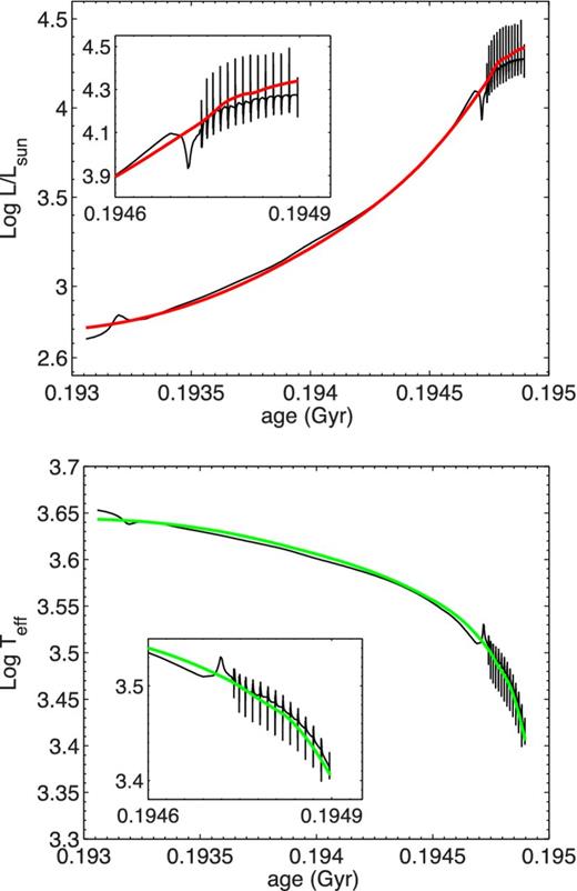
Evolutionary track for the AGB phase of a M = 4 Mȯ, Z = 0.02 stellar model. The top panel show the temporal variation of the luminosity, the bottom panel the evolution of the effective temperature. We display, superimposed on the track, the smooth approximations we have adopted.
Based on these considerations, the thermal pulses have been replaced by smoothed quantities in all evolutionary sequences that include the AGB phase. The procedure can be summarized as follows.
For each evolutionary sequence of fixed mass (and chemical composition) that includes the AGB phase, we have determined the start, duration and end of all the evolutionary phases of interest, to select the TP-AGB stage carefully.
As discussed in Weiss & Ferguson (2009), nearly all evolutionary sequences under consideration are followed to the end of the AGB phase, but for the highest masses (typically 5 and 6 Mȯ), because of numerical difficulties. In such cases, considering the rate of mass loss and the mass of the remaining envelope of the last model, an estimate of the number of missing pulses until the end of the TP-AGB is provided by Weiss & Ferguson (2009). We use this estimate to evaluate the total TP-AGB lifetime correctly for the few evolutionary sequences where this is required.
Using the matlab environment, we plot for each star the current mass (M/Mȯ), age (yr), mass-loss rate |$\dot{M}$|, luminosity log (L/Lȯ), effective temperature log Teff, gravity log g, central hydrogen mass fraction Xc and central helium Yc, core masses within the H- and He-burning shells Mc1 and Mc2 and the surface abundances Cs and Os, both as functions of the age and/or mass as appropriate. Making use of the Curve Fitting Toolbox (cftool) and locally weighted scatter-plot smoothing (Smooth Options Loess), we try to reproduce each of the above quantities by means of analytical fits. The method uses linear least-squares fit and second-order polynomials. The span parameter, which is the number of data points used to compute each smoothed value, is suitably varied. In locally weighted smoothing methods like Loess, if the span parameter is less than 1 it can be interpreted as the percentage of the total number of data points. For all the physical variables that do not oscillate, smoothing is not required and the span can be varied in such a way that the shape and the form of the original data are preserved.2
Once the smoothing procedure has been applied, we determine the start and the end of the E-AGB and TP-AGB phases and the oxygen-rich to carbon-rich transition. This is required for the interpolation between different values of the initial mass, to account correctly for the carbon-rich and oxygen-rich stages.
In order to include these new models of AGB stars in old isochrones and SSPs, we need to extend Weiss & Ferguson (2009)'s evolutionary models to masses as low as 0.6 Mȯ (at least). As already recalled, the Weiss & Ferguson (2009) data set extends only down to 1 Mȯ. To this aim, we extrapolate the Weiss & Ferguson (2009) stellar models gently down to 0.8 Mȯ, trying to scale all the physical variables (luminosity, Teff, time-scales) obtained for 1 Mȯ consistently. We follow a numerical technique similar to the one used for the smoothing procedure. For even lower masses that never reach the carbon-rich phase, a simple description is sufficient and we follow Bertelli et al. (1994) and Piovan et al. (2003).
Finally, we match the TP-AGB part of each sequence derived from the Weiss & Ferguson (2009) models to the end of the E-AGB phase of the corresponding (same initial mass and chemical composition) evolutionary tracks from Bertelli et al. (1994). Some details of this are given below.
3.3 Matching GARSTEC to Padua models
Both GARSTEC and Padua models, in addition to sharing the same assumptions for the mass-loss rates until the start of the TP-AGB phase, similar sources and treatment of opacities, the same metal mixture (Grevesse & Noels 1993) and many other common physical ingredients, are calculated with numerical codes that are descendants of the Göttingen code developed by Hofmeister, Kippenhahn & Weigert (1964).
This makes the match easier between evolutionary models from the main sequence to the E-AGB phase calculated by the Padua group and models for the TP-AGB phase calculated by Weiss & Ferguson (2009).
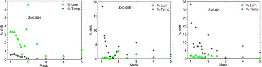
Relative variation Δf/f of effective temperature (stars) and luminosity (triangles) as a function of the initial stellar mass, between the Bertelli et al. (1994) and Weiss & Ferguson (2009) tracks at the end of the E-AGB phase. Results for three metallicities are displayed: Z ≃ ZSMC = 0.004, Z ≃ ZLMC = 0.008 (typical of LMC) and Z ≃ ZSN = 0.02 (solar neighbourhood).
3.4 The initial mass function
To calculate spectrophotometric properties of SSPs (SED, magnitudes, colours and luminosity functions) it is necessary to consider an IMF. There are several popular prescriptions in the literature. A few of them are listed in Table 1. For the purposes of our study, all IMFs are assumed to be constant in time and space. The IMFs in our list are Salpeter (Salpeter 1955, IMFSal), Larson (Larson 1998, IMFLar-MW, IMFLar-SN, with different parameters for the Milky Way disc and the solar neighbourhood (Portinari, Sommer-Larsen & Tantalo 2004)) Kennicutt (Kennicutt 1998, IMFKenn), the original IMF by Kroupa (Kroupa 1998, IMFKro-Ori), a revised and more recent version of this IMF by Kroupa (Kroupa 2007, IMFKrou-27), Chabrier (Chabrier 2003, IMFCha), Scalo (Scalo 1986, IMFSca) and Arimoto & Yoshii (Arimoto & Yoshii 1987, IMFAri). We refer either to the original sources or to to Piovan et al. (2011) for a detailed explanation of the main features of these IMFs.
Fraction of SSP total stellar mass at birth contained in several stellar mass ranges (see text for the definitions), as prescribed by several IMFs. The normalization constants are set to one. Columns are as follows: (1) the chosen IMF; (2) and (3) the corresponding lower and upper mass integration limits; (4) fraction contained in stars with mass larger than 1 Mȯ; (5) fraction contained in stars with M < 1 Mȯ, which do not contribute to chemical enrichment; (6) and (7) fraction contained in stars that contribute to the star–dust budget via the AGB and SN channel; (8) the total SSP mass MSSP at birth, in solar units.
| IMF | Ml | Mu | ζ>1 | ζ<1 | ζ1, 6 | ζ>6 | MSSP | |
|---|---|---|---|---|---|---|---|---|
| (1) | (2) | (3) | (4) | (5) | (6) | (7) | (8) | |
| Salpeter | IMFSalp | 0.10 | 100 | 0.392 | 0.6075 | 0.2285 | 0.1640 | 5.826 |
| Larson solar neighbourhood | IMFLar-SN | 0.01 | 100 | 0.439 | 0.5614 | 0.3130 | 0.1256 | 2.306 |
| Larson (Milky Way disc) | IMFLar-MW | 0.01 | 100 | 0.653 | 0.3470 | 0.3568 | 0.2962 | 3.154 |
| Kennicutt | IMFKenn | 0.10 | 100 | 0.590 | 0.4094 | 0.3883 | 0.2023 | 3.048 |
| Kroupa (original) | IMFKro-Ori | 0.10 | 100 | 0.405 | 0.5948 | 0.3016 | 0.1036 | 3.385 |
| Chabrier | IMFCha | 0.01 | 100 | 0.545 | 0.4550 | 0.3517 | 0.1933 | 0.025 |
| Arimoto | IMFAri | 0.01 | 100 | 0.500 | 0.5000 | 0.1945 | 0.3055 | 9.210 |
| Kroupa 2002–2007 | IMFKro-27 | 0.01 | 100 | 0.380 | 0.6198 | 0.2830 | 0.0972 | 3.134 |
| Scalo | IMFSca | 0.10 | 100 | 0.320 | 0.6802 | 0.2339 | 0.0859 | 4.977 |
Fig. 3 shows the mass dependence of the different IMFs and implicitly the mass interval covered by stars going through the TP-AGB and WD phases or ending in a SN explosion and thus contributing to the star–dust budget.
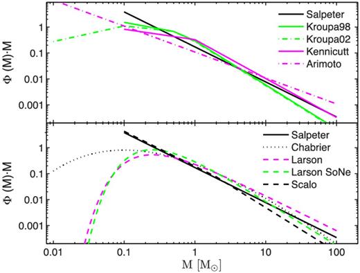
Fractional contribution to the total SSP mass budget of stars of different masses, as predicted by the labelled IMFs over the range where they are defined (see text for details). The widely used IMF by Salpeter (1955) is shown in both panels for the sake of comparison. Stellar masses are in solar units and all the IMFs in this case are normalized to a total SSP mass equal to 1 Mȯ.
4 THE NEW ISOCHRONES: RESULTS
We present here the sets of isochrones obtained with the new TP-AGB models. Each set contains isochrones for more than 50 age values, ranging from ∼3.0 Myr to 15 Gyr. The age range for the development of an AGB varies with metallicity according to
Z = 0.050: 7.78 ≤ log t ≤ 10.18;
Z = 0.020: 7.90 ≤ log t ≤ 10.18;
Z = 0.008: 8.10 ≤ log t ≤ 10.18;
Z = 0.004: 8.10 ≤ log t ≤ 10.18;
Z = 0.0004: 8.10 ≤ log t ≤ 10.18;
Z = 0.0001: 8.00 ≤ log t ≤ 10.18;
Fig. 4 shows a few selected isochrones for metallicities Z = 0.004 (typical for the SMC), Z = 0.008 (typical for the LMC) and Z = 0.02 (typical for the Sun and the solar vicinity), respectively. All other metallicities have similar HRDs. Important differences from Bertelli et al. (1994) arise obviously along the AGB phase, as shown in Fig. 5. The AGB phase for oxygen-rich envelopes is displayed with solid black lines, whereas the carbon-rich case with [C/O]>1 is displayed with dot–dashed lines (magenta in the online article). The beginning and end of each evolutionary phase is marked with a small star. Thanks to the new low temperature opacities (Weiss & Ferguson 2009), the isochrones now extend towards lower temperatures than in the old models. The enrichment of the C abundance at the surface of TP-AGB stars, accompanied by an important reduction of the effective temperature and the formation of a shell of dust surrounding the star (see below), are important steps forward that amply justify our efforts to calculate a library of stellar spectra for O- and C-rich dust-enshrouded AGB stars.
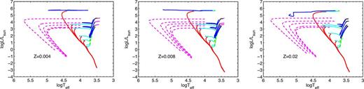
Isochrones with the new AGB models, from the zero-age main sequence to the stage of PN formation or central carbon ignition, depending on the initial stellar mass. Three metallicities are shown: Z = 0.004, typical of the Small Magellanic Cloud (left), Z = 0.008, typical of the Large Magellanic Cloud (middle), and Z = 0.02, typical of the solar neighbourhood (right). The isochrones are plotted for a few selected ages between 5 Myr and 15 Gyr.
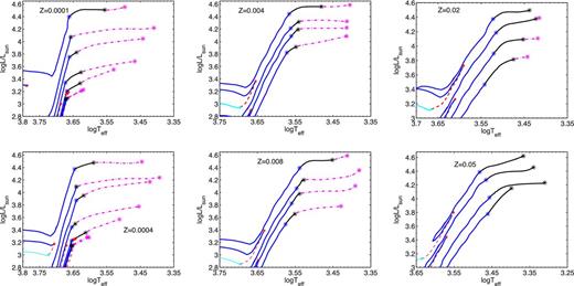
Isochrones in the theoretical HRD, centred on the E-AGB and TP-AGB phases, for the labelled metallicities. They are organized into three groups, from left to right: very low metallicities, Z = 0.0001 and Z = 0.0004 respectively (left); as in the left panels, but for Z = 0.004 and Z = 0.008 (central); and as in the previous panels, but for Z = 0.02 (solar value) and Z = 0.05 (right). Along each isochrone the end of the E-AGB phase is marked by a star (blue in the online article). The TP-AGB phase is in turn drawn as a solid black line when the envelope is oxygen-rich, and as a dot–dashed line (magenta in the online article) if carbon-rich.
Looking at the grids of isochrones for different metallicities, the following considerations can be made:
Solar and super-solar metallicities: Z ≥ 0.02. These stars are normally oxygen-rich at the surface, even if a late transition to the carbon-rich phase may take place due to the final dredge-up events, in agreement with observations (e.g. see van Loon et al. 1998, 1999, for more details). For solar metallicity, the transition occurs only in isochrones of intermediate ages and at very low Teff, during the final stages of the TP-AGB phase. In contrast, isochrones of supersolar metallicity show only oxygen-rich material at the surface. As expected, the youngest isochrones are the most extended in the HRD during the AGB phase. The TDU does not occur in the oldest isochrones of both metallicities and the TP-AGB phase is much shorter than the E-AGB phase.
Subsolar metallicities: 0.004 ≤ Z < 0.02. These stars show an extended carbon-rich phase, even at rather low ages. This is due to the onset of the ON cycle, which converts O into N, increasing the [C/O] ratio above 1 (Ventura, D'Antona & Mazzitelli 2002; Marigo et al. 2008). Furthermore, the carbon enrichment at the surface starts at higher effective temperatures (compared with solar-metallicity isochrones), because of lower molecular concentrations in the atmospheres (Marigo et al. 2008).
Low metallicities: Z < 0.004. All trends described for isochrones of moderate metallicities become more evident. The transition to a carbon-rich envelope starts at even higher effective temperatures and the majority of the isochrones show the C-star phase almost exclusively. Only few isochrones of intermediate ages have an oxygen-rich phase. Our results agree fairly well with those of Marigo et al. (2008), even though some marginal differences can be noticed. The agreement is ultimately due to the fact that both include opacities that depend on the [C/O] ratio. This is confirmed by the nearly identical effective temperatures of the AGB models and the similar behaviour of the oxygen-rich and carbon-rich stages with metallicity.
5 THE DUST-FREE SSPs
The most elementary population of stars is the so-called single (or simple) stellar population, made of stars born at the same time in a burst of star formation activity of negligible duration and with the same chemical composition. SSPs are the basic tool to understand the spectrophotometric properties of more complex systems like galaxies, which can be considered as linear combinations of SSPs with different compositions and ages, each of them weighted by the corresponding rate of star formation.
In more detail, the steps to calculate the SED of a SSP are as follows.
For a fixed age and metallicity, the corresponding isochrone in the HRD is divided into elementary intervals small enough to ensure that luminosity, gravity and Teff are nearly constant. In practice, the isochrone is approximated by a series of virtual stars, to which we assign a spectrum.
In each interval, the stellar mass spans a range ΔM fixed by the evolutionary speed. The number of stars assigned to each interval is proportional to the integral of the IMF over the range ΔM (the differential luminosity function).
Finally, the contribution to the integrated flux (at each wavelength) by each elementary interval is weighted by the number of stars and their luminosity.
The spectra of the virtual stars are taken from suitable spectral libraries, as a function of effective temperature, gravity and chemical composition. We employed the spectral library by Lejeune, Cuisinier & Buser (1998), based upon the Kurucz (1995) release of theoretical spectra, with several important implementations. For Teff < 3500 K, the spectra of dwarf stars by Allard & Hauschildt (1995) are included, whilst the spectra by Fluks et al. (1994), Bessell et al. (1989) and Bessell, Brett & Scholz (1991) are considered for giant stars. Following Bressan et al. (1994), for Teff > 50 000 K the library has been extended using blackbody spectra.
We have calculated grids of dust-free SSP SEDs of different ages, for the six values of metallicity and the nine different IMFs of Table 1, and derived magnitudes and colours for different photometric systems.
5.1 A comparison with the old dust-free SSPs
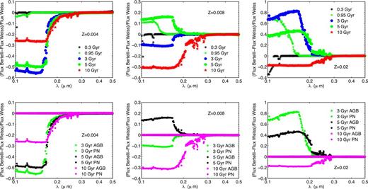
Upper panels: comparison between the integrated flux of our new SSPs and the old SSPs, as a function of λ, for the labelled ages and metallicities. Lower panels: as upper panels, but for both integrated and cumulative fluxes to the end of the AGB, for fewer selected ages. The left panels are for Z = 0.004, the central panels for Z = 0.008 and the right panels for Z = 0.02.
Other major differences appear in the IR spectral region, where AGB stars emit most of their light. This is shown by Fig. 7, which displays the ratios FRλ as a function of age at selected near-IR wavelengths, for different metallicities (Z = 0.004, 0.008 and 0.02). Given that we neglect the effects of circumstellar dust shells around the AGB stars, we expect that the cool M and C models emit most of the flux in the range ∼1–4 μm (dust would shift the emission towards longer wavelengths). The agreement between the two sets of SSPs is very good before the onset of the AGB phase and for great ages, where the differences amount to only a few per cent. As expected, when the AGB phase sets in at log t ∼ 8, differences are much larger. These can ultimately be ascribed to the different prescriptions for the TP-AGB phase in the Padua and GARSTEC models.
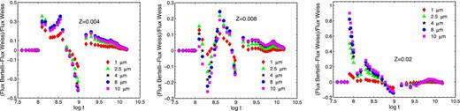
As in the upper panels of Fig. 6, but in this case we consider the residual flux ratios as a function of age for the labelled reference wavelengths λ. Three metallicities are shown: Z = 0.004 (left), Z = 0.008 (centre) and Z = 0.02 (right). The unit of time t is yr.
6 SSPs WITH CIRCUMSTELLAR DUST AROUND AGB STARS
It has long been known that low- and intermediate-mass AGB stars are amongst the main contributors to the ISM dust content. The previous evolutionary phases are not as important as dust factories: dust formation in RGB and E-AGB stars is poorly efficient because of the unfavourable wind properties and the low mass-loss rate (Gail et al. 2009). As for the calculation of SEDs, magnitudes and colours, the presence of dust shells is usually – with just a few exceptions (see for instance Bressan, Granato & Silva 1998; Mouhcine 2002; Piovan et al. 2003; Marigo et al. 2008) – not taken into account.
As TP-AGB stars are expected to form significant amounts of dust and therefore suffer self-obscuration and re-processing of their photospheric radiation, the effect of dust on their SEDs cannot be ignored (Piovan et al. 2003).
Dust formation in AGB stars has been modelled with increased accuracy over the years (Gail, Keller & Sedlmayr 1984; Gail & Sedlmayr 1985, 1987, 1999; Dominik, Sedlmayr & Gail 1993; Ferrarotti & Gail 2002, 2006; Gail et al. 2009) and we are now in the position to calculate the amount of newly formed dust in M stars, S stars and C stars (a sequence of growing [C/O] ratio). This ratio determines the composition of dust formed in the outflows (Piovan et al. 2003; Ferrarotti & Gail 2006; Gail et al. 2009). The oxygen-rich M stars ([C/O] < 1) produce dust grains mainly formed by refractory elements (generically named silicates) like pyroxenes and olivines, oxides and iron dust. Carbon-rich stars ([C/O] > 1) produce carbon dust; |$\rm {SiC}$| and maybe iron dust can form as condensate. In S stars ([C/O] ≈ 1), quartz and iron dust should form (Ferrarotti & Gail 2002). However, the carbon-rich or oxygen-rich phases dominate and for example the contribution of |$\rm {SiC}$| produced during the S-star phase can be neglected, compared with the |$\rm {SiC}$| produced during the C-star phase.
6.1 Modelling a dusty envelope
The problem of radiative transfer in the dusty shells that form around AGB stars has been addressed by many authors (see the classical review by Habing 1996, and references therein). The best approach would clearly be to couple the equations describing the radiative transfer through the dusty envelope with the hydrodynamical equations for the motion of the two components, dust and gas, taking into account the interplay between gas, dust and radiation pressure. For the purposes of this work, it is however enough to limit ourselves to solving the problem of radiative transfer through the envelope (Ivezic & Elitzur 1997; Rowan-Robinson 1980). Indeed, our purpose is to build a library of dusty SEDs to determine the effects of dust around AGB stars, not to study the dynamical behaviour of the outflows.
6.1.1 The optical depth
6.1.2 Mass-loss
6.1.3 Dust-to-gas ratio
Another important parameter of equation (14) is the dust-to-gas ratio δ. In Piovan et al. (2003), the dust-to-gas ratio was obtained by simply inverting a relation between velocity, luminosity and dust-to-gas ratio based upon the results by Habing et al. (1994).
6.1.3.1 Oxygen-rich M-stars.
6.1.3.2 S stars.
6.1.3.3 Carbon-rich C stars.
7 THEORETICAL SPECTRA OF O- AND C-RICH STARS
Our goal is to calculate spectra modified by the effect of the dust shells around the AGB stars. The ideal approach would be to generate the corresponding SED for each AGB model and use it to derive magnitudes and colours in a given photometric system. However, this way of proceeding, which was occasionally adopted by Piovan et al. (2003), is very time-consuming. It requires solving the radiative transfer problem on a star-by-star basis: it can be applied only if the number of models is small. In the present study, we follow a different approach. We first set up two libraries of dust-enshrouded AGB spectra, one for O-rich and the other for C-rich objects, covering the full parameter space spanned by our AGB models. Interpolations among the library SEDs will provide the spectrophotometric properties of the AGB section of our isochrones. Each library contains 600 spectra. The parameters have been grouped according to the following criteria.
The optical depth. τ is derived from equation (14) using the appropriate physical parameters that describe the central star and the surrounding dust shell. For each group (C stars and M stars), we calculate 25 optical depths, going from 0.000045 to 40 (Groenewegen 2006), at a suitable reference wavelength of the MIR, for the chemical mixture that forms the dust.
The SED of the central star embedded in the dust-shell. The total luminosity is not required, a normalized flux λFλ in some arbitrary units being sufficient. The following SEDs for the central stars are adopted: for the oxygen-rich stars we use the SEDs of the Lejeune, Cuisinier & Buser (1997) library, which also includes semi-empirical spectra of cool M stars by Fluks et al. (1994); for the C stars we select a suitable number of SEDs from the Aringer et al. (2009) models of dust-free C stars. For the M stars, we adopt six values of temperature (2500, 2800, 3000, 3200, 3500 and 4000 K), but no specification is made for the gravity, because the sample of Fluks et al. (1994) contains empirical spectra. For the library of C stars we adopt six values of temperature (2400, 2700, 3000, 3200, 3400 and 3900 K); see also Aringer et al. (2009). We consider two values for the [C/O] ratio, namely [C/O] = 1.05 and [C/O] = 2. Finally, for the input mass, gravity and metallicity we use M = 2 Mȯ, log g = 0.0 and Z = Zȯ.
The composition of the dust in the outer envelope.
C stars. Several types of dust grains in carbon-rich AGB stars have been detected by observations: the three main types are amorphous carbon (AMC), silicon carbide (SiC) and magnesium sulphide (MgS). In our models the presence of MgS has been neglected. MgS was first proposed as a candidate to explain the 30-μm feature in evolved C stars by Goebel & Moseley (1985) and this hypothesis has been strengthened by theoretical and observational analyses (see Zhukovska & Gail 2008, for more details). However, according to recent studies, to account for the feature in a typical C-rich evolved object one would require a much higher MgS mass than available (Zhang, Jiang & Li 2009). Also, MgS causes a mismatch between predicted and observed spectral features (Messenger, Speck & Volk 2013). In addition, the 30-μm feature is not ubiquitous: it is difficult to determine the ranges of stellar mass and mass loss where the feature should be included (Zhukovska & Gail 2008); therefore, in conclusion, we decide to ignore MgS. With respect to AMC and SiC, we rely on the results by Suh (2000), who derived new opacities for the AMC that are consistent with the Kramers–Kronig dispersion relations and reproduce the observational data. The models improve upon previous studies (Blanco et al. 1998; Groenewegen et al. 1998) and are characterized by two components, SiC and AMC. AMC and SiC influence the outgoing spectrum in different ways: whilst the effects of AMC propagate over the whole spectrum, those of SiC are limited to the 11-μm feature, as indicated by the observations. Lorenz-Martins & Lefevre (1994) and Groenewegen (1995) suggest that the ratio SiC to AMC decreases at increasing optical depth of the dusty envelope. According to Suh (1999), for optically thin dust shells (|$\tau _{{\rm 10}} \le \rm {0.15}$|, where τ10 is the optical depth at 10 μm), the strong 11-μm feature requires about 20 per cent of SiC dust grains to fit the observational data; for dust shells with intermediate optical thickness (0.15 ≤ τ10 ≤ 0.8), about 10 per cent SiC dust grains are needed, whereas for shells with larger optical depths, where the 11-μm feature is either much weaker or missing at all, no SiC is required. The optical constants of |$\alpha \rm {SiC}$| by Pégourié (1988) are adopted to calculate the opacity of SiC and according to the above considerations we take two extreme compositions: the first one has 100 per cent AMC only, whereas the second one has 80 per cent AMC and 20 per cent SiC. The reference optical depth has been chosen at 11.33 μm for the 100 per cent AMC mixture and at 11.75 μm for the 80 per cent AMC and 20 per cent SiC mixture (Groenewegen 2006).
M stars. In the circumstellar environment of M stars, a wide number of dust grains is formed and a condensation sequence has been proposed by Tielens (1990). At increasing mass loss, the dust composition changes from aluminium and magnesium oxides, rich at low |$\dot{M}$|, to a mixture with both oxides and olivines and finally to a composition dominated by the silicates, with amorphous silicates and crystalline silicates at high |$\dot{M}$|. This sequence seems to be able to reproduce the changes observed in the shape of the 10-μm feature. Even if this scheme is still a matter of debate (van Loon et al. 2006), it is consistent with the observations of different types of stars at different metallicities (Dijkstra et al. 2005; Heras & Hony 2005; Blommaert et al. 2006; Lebzelter et al. 2006). We adopt the above sequence as a plausible scenario for the condensation of dust in oxygen-rich stars. Three possible compositions are included: (1) pure Al2O3 with optical properties taken from Begemann et al. (1997); (2) mixed composition with 60 per cent Al2O3 and 40 per cent silicates, with the optical properties taken from David & Pegourie (1995); (3) 100 per cent silicates for high mass-loss rates, with two possible choices, i.e. either a complete composition with optical properties from David & Pegourie (1995) for comparison with Groenewegen (2006) or a more elaborate description based upon Suh (1999, 2002). The latter author adopted different silicates opacities at varying 10-μm features, namely cold and warm silicates. The model was then refined by Suh (2002), taking into account crystalline silicates through the so-called crystallinity parameter α, because in many AGB stars with high mass-loss rates Infrared Space Observatory (ISO) high-resolution observations reveal the presence of prominent bands of crystalline silicates, like enstatite (|$\rm {MgSiO}_{3}$|) and forsterite (|$\rm {Mg}_{2}\rm {SiO}_{4}$|) (Waters et al. 1996; Waters & Molster 1999). The adopted opacity functions for these latter are taken from Jaeger et al. (1998). Following Piovan et al. (2003), we adopt here α = 0.1 for stars with low mass-loss rates and moderately optically thick shells (τ10 < 15), whereas for oxygen-rich stars with high mass-loss rates and very thick shells (τ10 > 15) we prefer the value α = 0.2. Finally, in all models the relative contents of enstatite |$\left( \rm {MgSiO}_{3}\right)$| and forsterite |$\left( \rm {Mg}_{2}\rm {SiO}_{4}\right)$| are the same as in Suh (2002). We take also into account the recent results by McDonald et al. (2011). They found that metallic iron seems to dominate the dust production in metal-poor oxygen-rich stars. We therefore adopt a 100 per cent iron mixture to simulate the envelope of metal-poor stars surrounded by a thin dust shell. The optical properties of iron are taken from Ordal et al. (1988). The following reference wavelengths are adopted for the grid of τ: 11.75 μm for both pure aluminum oxides and oxides plus silicates and 10.20 μm for both pure silicates cases. All the above opacities are used as input for dusty. This radiative transfer code then applies Mie theory to calculate scattering and absorption efficiencies by a homogeneous spherical sphere. The grain size distribution is chosen between the options available in dusty (Ivezic & Elitzur 1997). In particular, we adopt single-size grains with dimension a = 0.1 μm (see Piovan et al. 2003 for more details about this choice). An analytical dust density profile, suitable for the modelling of AGB stars, is also selected from the available options. This profile is appropriate in most cases and offers the advantage of a much reduced computational time (see the dusty manual).3 The envelope expansion is driven by radiation pressure on the dust grains.
The temperature T at the inner boundary of the dust shell. For this parameter we assume either 1000 or 1500 K, depending on the type of dust (Piovan et al. 2003).
Finally, we comment on the luminosity of the central star. For C stars, we keep the luminosity specified by Aringer et al. (2009). Given that Fluks et al. (1994) does not specify the luminosity of the M stars producing the empirical spectra, but gives only the specific intensity, we fix the luminosity of the M stars at L = 3000 Lȯ. The library of dusty stellar spectra is therefore calculated for a fixed luminosity of the underlying objects. This is not a problem, because the luminosity does not affect the solution of the radiative transfer (Ivezic & Elitzur 1997) and the shape of the outgoing SEDs. The resulting flux is scaled to the real luminosity of the AGB star we are considering.
Fig. 8 displays the SEDs of O-rich AGB stars of our template library for four values of the optical depth. The input parameters are Teff = 2500 and L = 3000 Lȯ for the central star, optical depths τ = 0.0224, 0.2081, 1.306 and 30.0 and dust composition according to the second prescription for oxygen-rich stars (60 per cent Al2O3 and 40 per cent silicates). The lower left panel shows the results for two different gravities (log g = −1.02 and log g = 0.5) of the input spectrum from the Fluks et al. (1994) compilation. For the sake of clarity, the two SEDs are artificially shifted by a small amount, otherwise the two spectra would be coincident. Indeed, as expected and tested, there is no dependence on gravity in the Fluks et al. (1994) spectra. The stellar features in the UV–optical–near-IR region disappear with increasing optical depth and an increasingly featureless SED appears: this is ultimately due to the smooth optical properties of the selected composition. The stellar light is shifted more and more towards longer wavelengths; for the lowest optical depths the input and output spectra are almost coincident, while the effect of dust is apparent for the largest values of τ. In the lower panels we show the fractional contribution of the attenuated input radiation to the total flux (labelled as Att – solid lines); the fractional contribution of the scattered radiation to the total flux (labelled as Ds – dot–dashed lines) and finally the fractional contribution of the dust emission to the total flux (labelled as De – dotted lines). As expected, at increasing optical depth τ, (i) the fraction of not attenuated or scattered light escaping the dust shell decreases and (ii) the dust contribution becomes significant at τ ∼ 0.2 and dominant at τ ∼ 1.
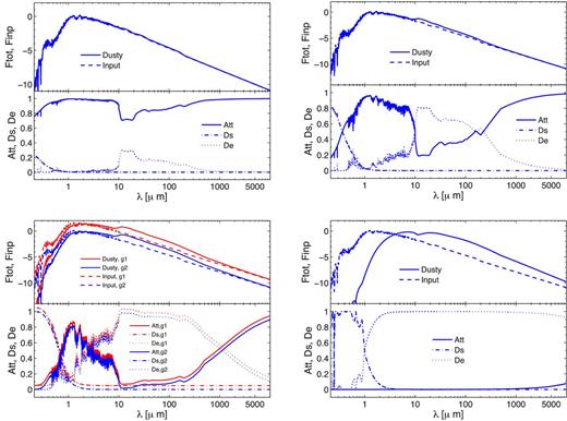
Dust-enshrouded spectra for AGB stars obtained with our modified version of the radiative transfer code dusty. The input parameters are M-type AGB stars with Teff = 2500 and L = 3000 Lȯ and an oxygen-rich surface composition with 60 per cent Al2O3 and 40 per cent silicates. The SEDs for four values of the optical depth are shown: τ = 0.0224 (upper left), τ = 0.2083 (upper right), τ = 1.306 (lower left) and τ = 30.0 (lower right). The lower left panel shows the results for two different gravities of the input spectra. More details are given in the text.
Finally, Fig. 9 shows a sequence of obscured spectra of AGB stars at increasing optical depth, both for O-rich (top panel) and C-rich (bottom panel) stars. It is evident that the SEDs progressively shift towards longer wavelengths with increasing τ. The spectra with 100 per cent AMC dust composition represent a limiting case with no SiC feature at 11.3 μm. It is worth noticing that for the oxygen-rich stars, when the optical depth is very high, the silicate feature at 9.7 μm appears in absorption, as indicated by the observational data (Suh 1999, 2002).
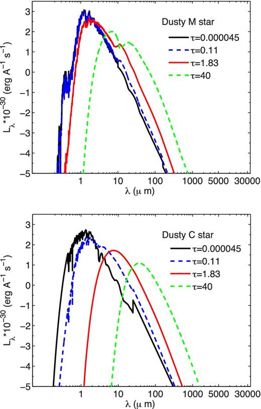
Dust-enshrouded AGB spectra for various optical depths for oxygen-rich M stars (top) and carbon-rich C stars (bottom).
8 SEDs AND COLOURS OF SSPs WITH DUST-ENSHROUDED AGB STARS
With our new isochrones and library of dust-enshrouded AGB stars, we have calculated the SEDs of SSPs. Fig. 10 displays the SEDs with (solid lines) and without (dashed lines) dust-enshrouded AGB stars for different ages and metallicities Z = 0.004 and Z = 0.05, respectively. Ages range from 0.1 to 2 Gyr and correspond to young and intermediate-age SSPs. The effect of the dust-enshrouded AGB stars is remarkable and cannot be neglected in the region from NIR to FIR. Fig. 11 shows the SEDs for high ages from 6–10 Gyr, for metallicities Z = 0.008 and Z = 0.05, respectively. For high ages, the effect of dust-enshrouded AGB stars is small, mainly because of the short duration of the AGB phase (only a few thermal pulses) due to the low total mass along the AGB. Only for the highest metallicity Z = 0.05 does the dust surrounding AGB stars have some effect on the SED. Another example of the effect of the dust shells around AGB stars is shown by Fig. 12, which compares the new and old SEDs for a few selected ages and for three metallicities, Z = 0.0001, Z = 0.008 and Z = 0.05. Similar results are found for all remaining metallicities.
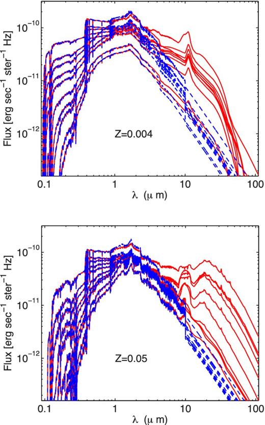
SEDs (Fν versus λ) for SSPs with ages from 0.1–2 Gyr. The case with dusty circumstellar envelopes around AGB stars is displayed as solid lines (red in the online article), while results without dust are plotted with dotted lines (blue in the online article). Ages range from the largest (bottom) to the smallest (top) values (2.0, 1.5, 0.95, 0.8, 0.6, 0.4, 0.325, 0.25, 0.15, 0.1 Gyr). The metallicity is Z = 0.004 (top) and Z = 0.05 (bottom).
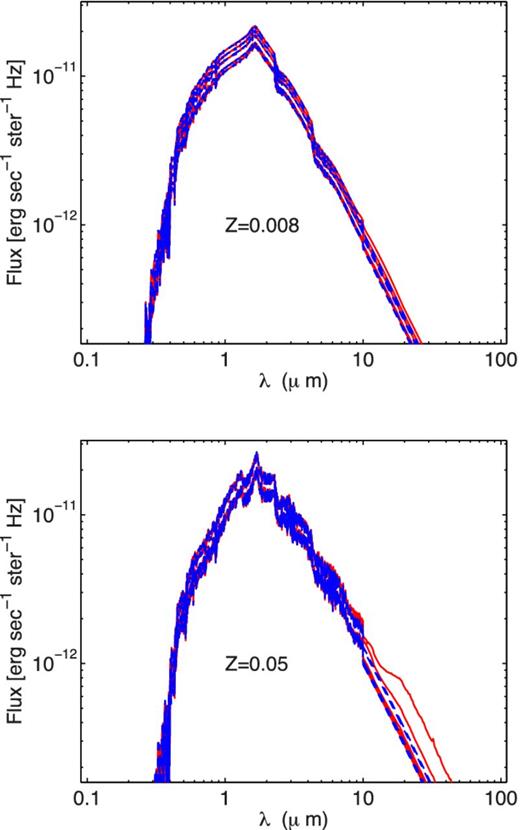
SEDs (Fν versus λ) for the SSPs with Z = 0.008 (top panel) and Z = 0.05 (bottom panel). Red solid lines correspond to models including dusty circumstellar envelopes, and blue dotted lines to SSPs without dust. From bottom to top the displayed ages are: 6, 7, 8, 9 and 10 Gyr.
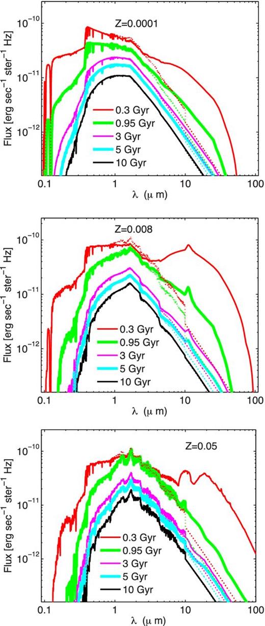
Detailed comparison of SEDs for old SSPs (dotted lines) and new SSPs (solid lines) for the labelled ages and metallicities. Three metallicities are shown: Z = 0.0001 (top), Z = 0.008 (middle) and Z = 0.05 (bottom).
The old spectra without dust shells do not extend into the NIR and FIR, but decline sharply at wavelengths longer than about 3–4 μm. The spectra of the new SSPs, instead, extend towards long wavelengths and the amount of flux in the MIR and FIR is significant. Differences start at about 1 μm; in the IR range up to 3–4 μm, the flux of dusty SSPs is lower than the old one, due to the fact that dusty envelopes shift the emission of M and C stars towards longer wavelengths. It is worth noticing the evolution of the features of silicon carbide at 11.3 μm and amorphous silicate at 9.7 μm at different metallicities. The amount of energy shifted to longer wavelengths is larger for low ages, because of a more massive and luminous AGB. Considering the different metallicities, we note the following effects.
Z = 0.0004 and Z = 0.0001: for stars of very low metallicity the TDU is particularly efficient during the AGB phase in enriching the surface with 12C and other products of He burning. These stars display a C-rich surface for most of their evolution. The presence of dusty C-rich stars in young SSPs leads to featureless SEDs dominated by amorphous carbon. The small amounts of metals in the envelope inhibit high optical depths and the amount of radiation re-emitted in the MIR/FIR region is smaller than in the case of higher metallicities.
Z = 0.004 and Z = 0.008: for most of the age range covered by the models, the spectrum does not show the features due to amorphous and crystalline silicates, because C stars dominate (the 11.3-μm feature of SiC is indeed prominent). This is quite different from the results by Piovan et al. (2003), where the oxygen-rich phase at these metallicities played an important role and a significant evolution of the MIR features was present. In Piovan et al. (2003), C stars dominated for low ages, whereas for intermediate ages (around 3 Gyr) O stars of low optical depth contributed to the integrated spectrum and the 9.7-μm feature could be seen in emission. Finally, for even higher ages high optical depth O stars dominated, such that the spectrum became more articulated and the features due to crystalline silicates started to appear in the IR. All this no longer occurs (for metallicities in this range), simply because the evolution of the [C/O] ratio in the Weiss & Ferguson (2009) models of AGB stars leads to a different path. Furthermore, it must be noted that, compared with Piovan et al. (2003), the amount of flux shifted towards longer wavelengths is generally smaller. This is due to the lower optical depths, now more realistically linked to the composition and mass loss of the underlying star. Finally, the present optical depths agree well with those of Groenewegen (2006) for similar mass-loss rates.
Z = 0.02: for the lowest ages, C stars appear in a narrow luminosity range (Fig. 5) and the stars at the AGB tip, with the highest mass-loss rate and the highest optical depth, are O stars. The SSP spectrum is dominated by the 9.7-μm feature, which appears in emission and not in absorption, as expected in envelopes with rather small optical depths. No features of crystalline silicates show up in the spectrum, because according to the models by Suh (2002) much higher optical depths would be required.
Z = 0.05: AGB stars with super-solar metallicities display only oxygen-rich surfaces (Fig. 5) and do not reach the carbon-rich phase in the models by Weiss & Ferguson (2009). At 0.3 Gyr and for low ages (see Fig. 12), the SSP spectra display both amorphous silicates (at ∼ 10 μm) and features due to crystalline silicates (∼30 μm) because of the high optical depths.
8.1 SSP colours
SEDs and colours of SSPs have a strong dependence on age, metallicity and the presence of dust shells around the AGB stars. This is clearly demonstrated by Figs 13, 14 and 15 for the [B − V], [V − K] and [J − 8 μm] colours. The age range considered covers the onset of the AGB phase until very high ages, when the contribution of AGB stars to the integrated flux is very low. As well known, age and metallicity – this latter enhanced by the effects of AGB dust shells – drive the evolution of the SSP colours.
![Integrated [B − V] colour of SSPs as a function of age, in the range 0.1–15 Gyr, for the whole metallicity grid. Solid lines denote SSPs with dust-free AGB stars, dashed lines colours including dust-enshrouded AGB stars. The unit of time t is yr.](https://oup.silverchair-cdn.com/oup/backfile/Content_public/Journal/mnras/436/3/10.1093_mnras_stt1778/2/m_stt1778fig13.jpeg?Expires=1716402345&Signature=KPbMoDnbvn~ia6YzE8chN31BF7RUZZeJ2F7uQaGlTVYl2p2y30InC5UtV5Hp0HbMNbiwS7amI9XUbNTJavDslH2nnAgXVWD5KIJHqp3AKqd-luu2rZ536keb2nVC90cog3q9KFk4LJ30C~f8gFGzzYoZLtTQzA2MIJD9BL9Hi0ubD9mIW~HkXbPvcSRXrQjUrpQ0Bkqj-In9YIMdtkl9TyOB~3lzKlzVULNOc7S9zlCsUxUw8Tevq67dHPWDP~GFB6zEC0H88Dr8vl4Q-U0EVMCXHkDMgfHphPqKxDZ-GCyng8-CwseP8KrwNeKq2Wj5MREh696TPuRXXrNm3ypNdg__&Key-Pair-Id=APKAIE5G5CRDK6RD3PGA)
Integrated [B − V] colour of SSPs as a function of age, in the range 0.1–15 Gyr, for the whole metallicity grid. Solid lines denote SSPs with dust-free AGB stars, dashed lines colours including dust-enshrouded AGB stars. The unit of time t is yr.
![As Fig. 13, but for the integrated [V − K] colour.](https://oup.silverchair-cdn.com/oup/backfile/Content_public/Journal/mnras/436/3/10.1093_mnras_stt1778/2/m_stt1778fig14.jpeg?Expires=1716402345&Signature=iCBjpK4qS78GnQmaLOi1khkCSKNCHgwNwjWQNf5Wv0PkG8gVRp~lHINbt7BejM2ZAStCTtmHCsa8Dz6obMJjQ5re1zCASwZHLd309aU7cgSTIUN-9KSAVK3Rkb5S1PpoRqx4f8QLJmPwnvQs0SGcEAxCVdjshC7FaYWsl5MrQ4-XsS81JeJs4Wrt7ZcJTS6hChkWUVxyUMU6Q~gmSIL4YwXGlW9h01lfHnj9nBz7p6kXt09wZ-3~buRNNsAC5LB1DbUUHBNDRwL9EY4ttPm4yW8ourGLNIv6boUr88uYG7FE2fa4KvmNKhPUiKCKPzh2jTIvLe0Ktq3MrDHWRdY73g__&Key-Pair-Id=APKAIE5G5CRDK6RD3PGA)
![As Fig. 13, but for [${J} - \rm {8}$ μm].](https://oup.silverchair-cdn.com/oup/backfile/Content_public/Journal/mnras/436/3/10.1093_mnras_stt1778/2/m_stt1778fig15.jpeg?Expires=1716402345&Signature=dR9PYiLmaoOzXBGePxl9Z-t9vwlx6uY6oBdKIVRet-8Nj9mnDSzEiSS75dmiD0utcttNkZmSbz5IwUzBICWV1t3nqhOD-HktWor~I7gqBQJJN16kJHG05gcGwua6gv3~FUgwuS9OyRGCx05y1LqYT5pUOnE-v0ZEhdjCiUDh7d2VyohC1glPV8Qp1O-~ae-TUzPWFP-kbO-7TAUR5~MJc6T7~yQ4zDEB8gbWoFugTWP5Fp6KUTAbySWS6yWHhKjj541Wcvl6k8bYcPycvrWebeD-K34OG-1hR8-hAu5T6v8ZFOBr2zNk4pgvKb508wwPjWNGoun~HIBPwfrqWh~XXA__&Key-Pair-Id=APKAIE5G5CRDK6RD3PGA)
The peak emission of the central AGB stars surrounded by dust shells is at around 1–2 μm; the dust shifts the flux from J, H and K bands to longer wavelengths. This effect is stronger at shorter wavelengths (J band) than at the longer ones (e.g. K band). It is the combination of this effect together with the exact position of the emission peaks of the central stars that determines the increase in IR magnitudes. Depending on the age and metallicity of the population, the net effect is that sometimes the J magnitude increases more than the K magnitude, while in other cases the opposite effect is true. It is in the Spitzer 8-μm passband that we mostly see the radiation emitted by dust around AGB stars. Even the coolest AGB star would provide a negligible contribution to that band if the dust shells were ignored. For the [V − K] colour, dust mainly makes the K magnitude fainter and affects the V flux only slightly, producing overall bluer colours. The effect of dust is small in the UV/optical passbands (see Fig. 13) and the [B − V] colours are practically unaffected by the presence of the dust surrounding AGB stars.
8.2 SEDs and colours of SSPs for variations in the IMF
Recalling the definition of the monochromatic flux emitted by an SSP of age t and metallicity Z, the choice of an IMF implies that along the corresponding isochrone, between Ml and Mu(t) (the most massive living stars at that age), the relative number of stars per mass interval dM is defined. The mass range spanned by all evolutionary stages beyond the main sequence turn-off decreases from a few solar masses to a few hundredths of a solar mass as the age increases from very young (a few Myr) to very old (a few Gyr). This means that, save for very young SSPs, changing the IMF has little impact on the integrated magnitudes and colours of SSPs. Main-sequence stars that are one or two magnitudes fainter than the turn-off contribute significantly to the SSP mass but little to magnitudes and colours.
In relation to this, we recall that the various IMFs do not have the same Ml and do not predict the same percentages of stars and hence stellar mass in different mass intervals. Looking at the entries of Table 1, IMFKro-27, IMFLar-MW, IMFLar-SN, IMFCha and IMFAri are all defined down to a lower mass limit of 0.01 Mȯ, whereas the remaining ones have a lower mass limit of 0.1 Mȯ (Piovan et al. 2011). Some IMFs, like IMFKro-Ori and IMFSca, predict a number fraction of massive stars – including SNe – that is much smaller than the number fraction of AGB stars. Others, like IMFLar-MW, IMFKenn and IMFCha behave in a different way and, even if again they predict a fractional mass of AGB stars higher than that of SNe, the relative contribution of SNe is much more significant. Only for the peculiar IMFAri is the trend reversed, with SNe outnumbering AGB stars. The difference in number ratios of stars going through the AGB to stars that become SNe has two effects. First, we expect that for the IMFs with a greater AGB mass fraction the effect of AGB circumstellar dust on magnitudes and colours is more significant than in the other cases. Secondly, the IMF choice affects the amount of dust injected into the ISM. Before the main process of dust formation happens in the ISM, the partition between AGB and SNe drives the amounts of star dust injected into the ISM (Zhukovska et al. 2008; Piovan et al. 2011). In each generation of stars, the dust production by either SNe or TP-AGB stars therefore depends on the IMF.
Small differences in the IMFs shown in Fig. 3, especially for M > 10 Mȯ, have a significant effect on young SSPs. To illustrate this point we calculate the SEDs of SSPs with different chemical composition and age, for all the IMFs listed in Table 1 and for metallicities Z = 0.004 and Z = 0.02. The SEDs are presented in Fig. 16 for three selected ages, namely 10, 100 and 300 Myr, and are limited to a metallicity of Z = 0.02 (similar results are found for the other metallicities). First of all, the SEDs run nearly parallel for the full wavelength range of interest. We therefore expect the ratio of the flux Fλ(λ, IMF1)/Fλ(λ, IMF2) between the SEDs of any two IMFs to remain similar over most of the spectrum. This is shown by the entries of Table 2, which lists the fluxes predicted by our IMFs for the three selected ages presented in Fig. 16, two metallicities and a total mass MSSP = 1 Mȯ, normalized to the values predicted by the Salpeter IMF. For each case, the minimum and maximum flux ratios obtained across the wavelength range from 0.1–100 μm are displayed.

Comparison between the new dusty SEDs at varying age and IMF. The metallicity is Z = 0.02. Three ages are considered: t = 10 Myr (left), 100 Myr (middle) and 300 Myr (right). Each line corresponds to a different IMF, according to the line-style and colour code of Fig. 3. Very similar curves are found for all other metallicities.
Ratios of the integrated fluxes predicted by several IMFs to those of the Salpeter IMF. Two metallicities are considered: Z = 0.004 and Z = 0.02. Three ages are displayed: t = 10, 100 and 300 Myr. All SSP fluxes are normalized to a total SSP mass of 1 Mȯ. Given that for a given IMF, Z and age the ratios depend on the wavelength, we display for each case the minimum and maximum values.
| Age (Myr) | 10 | 10 | 100 | 100 | 300 | 300 | |
|---|---|---|---|---|---|---|---|
| Metallicity Z | 0.004 | 0.02 | 0.004 | 0.02 | 0.004 | 0.02 | |
| Larson solar neighbourhood | IMFLar-SN | 0.87–0.99 | 0.90–1.05 | 1.33–1.41 | 1.29–1.42 | 1.46–1.55 | 1.44–1.54 |
| Larson (Milky Way disc) | IMFLar-MW | 1.79–1.81 | 1.77–1.81 | 1.69–1.71 | 1.67–1.72 | 1.59–1.66 | 1.60–1.68 |
| Kennicutt | IMFKenn | 1.22–1.30 | 1.24–1.34 | 1.50–1.57 | 1.49–1.58 | 1.58–1.67 | 1.58–1.67 |
| Kroupa (original) | IMFKro-Ori | 0.61–0.70 | 0.63–0.76 | 1.00–1.09 | 0.97–1.04 | 1.13–1.27 | 1.10–1.26 |
| Chabrier | IMFCha | 1.18–1.33 | 1.22–1.38 | 1.57–1.61 | 1.58–1.61 | 1.58–1.62 | 1.59–1.63 |
| Arimoto | IMFAri | 1.80–1.57 | 1.48–1.74 | 1.10–1.01 | 1.00–1.14 | 0.86–0.96 | 0.87–0.98 |
| Kroupa 2002–2007 | IMFKro-27 | 0.66–0.76 | 0.68–0.82 | 1.08–1.18 | 1.05–1.19 | 1.22–1.37 | 1.19–1.35 |
| Scalo | IMFSca | 0.42–0.48 | 0.43–0.51 | 0.69–0.74 | 0.66–0.75 | 0.77–0.86 | 0.75–0.85 |
Looking at the entries of Table 2, we see that IMFAri and IMFLar-MW predict the largest SSP fluxes for the lowest age, followed by IMFKenn (IMFCha is practically coincident with IMFKenn), in agreement with what is suggested by Fig. 3. IMFAri and IMFLar-MW indeed present the greatest fractional mass contribution of high-mass stars. At SSP ages t = 100 and 300 Myr, IMFKenn, IMFLar-MW and IMFCha have the highest flux ratio (as expected from the entries of Table 1). These IMFs predict the greatest fraction of stars with mass between 1 ≤ Mȯ < 6. The same trend is visible for Z = 0.004. For the ages considered, IMFSca predicts the lowest SSP flux. It has a very small fraction of massive stars, favouring low-mass stars in comparison with the other IMFs: in fact, 68 per cent of the mass is contained in stars with M < 1 Mȯ (see Table 1). This causes, as discussed, a lower integrated flux (see the panels of Fig. 16).
We now turn to colours like [V − K] and [J − 8 μm] that are affected by AGB stars. Fig. 17 shows that the effect of the IMF is stronger for the lowest ages where an AGB is present, up to 0.2 mag in [V − K]. For the highest ages, changing the IMF does not affect the integrated colours of the SSPs significantly. For both metallicities (Z = 0.02 and Z = 0.004 – the remaining ones behave in the same way), when AGB stars appear at approximately log t = 8, the IMFLar-MW predicts the reddest [V − K] colour, whereas the IMFKro-27 predicts the bluest one. This is due to the combined effect on the K band of the varying fractional mass of AGB stars and circumstellar dust. The former effect dominates and makes the colour redder; it is increasing when going from IMFKro-27 to IMFLar-MW. The effect of circumstellar dust effect is less important and opposite. As we have seen, while the V magnitude is not affected by circumstellar dust, the K magnitude is influenced, producing bluer colours (see Fig. 14). In the case of the [J − 8 μm] colour, different IMFs do not change its evolution appreciably and the effect is even smaller than in [V − K].
![Theoretical [V − K] and [J − 8 μm] colours as a function of age (from 0.1–15 Gyr) for the labelled metallicities and the two IMFs that cause the most extreme variations: results for the other IMFs discussed in this article lie between the lines displayed. Colour and line style for the results with different IMF are as in Fig. 3. Time t is again in yr.](https://oup.silverchair-cdn.com/oup/backfile/Content_public/Journal/mnras/436/3/10.1093_mnras_stt1778/2/m_stt1778fig17.jpeg?Expires=1716402345&Signature=gTvZ8pIsy4RKGpqOcr-0Olf4NGqOSp1cvJTR0hx2CTiTXY-XF7~gdPK~8DTf1K3l-AUicfBUtMAnDe7QksQZXKpWwHy5dHqEVgdjSeTyI~kms68j3lx5YH-h5w9-hhd0e7i-ZKNJeO8w2e7Jfd58wZkKcswOqV9LPIaqljNzzPvuszW4e-lwz9LBC2Uf5FXL9AjBOVQWKi5BRxPCs1vSgNjEoWBuoFZCupBNeo7vBmXALACJSM4OXcMAN~pXJ3ZJ1q2R-eaEMZXO~V3Qd93m6E4R6-cbf5SmCuwFXb-M1h187svP9hFPsKi-pWhZw2zQD8C3qpkzLHiM9FSz8jevWg__&Key-Pair-Id=APKAIE5G5CRDK6RD3PGA)
Theoretical [V − K] and [J − 8 μm] colours as a function of age (from 0.1–15 Gyr) for the labelled metallicities and the two IMFs that cause the most extreme variations: results for the other IMFs discussed in this article lie between the lines displayed. Colour and line style for the results with different IMF are as in Fig. 3. Time t is again in yr.
Finally, the effect of the IMF on the SED of SSPs does not depend appreciably on the chosen metallicity. This is shown by the entries in Table 2: the ratios are almost identical for both metallicities at all ages considered.
9 COMPARING THEORETICAL RESULTS WITH OBSERVATIONS
The key quantities to determine from the analysis of a stellar system are the age and metallicity distribution of the parent stars, to reconstruct the star formation and chemical enrichment history of the whole population. A widely used method to determine the age and metallicity of unresolved stellar systems is to compare their observed colours with the predictions of EPS models (see Bressan et al. 1994; Tantalo et al. 1998; Bruzual & Charlot 2003; Buzzoni 2005; Piovan, Tantalo & Chiosi 2006a; Piovan et al. 2006b; Galliano, Dwek & Chanial 2008; Popescu et al. 2011, to mention just a few). If instead the stellar populations can be resolved into single stars, the star-by-star EPS technique enables one to build synthetic CMDs (Chiosi, Bertelli & Bressan 1986; Bertelli et al. 1994; Aparicio & Gallart 2004; Chung et al. 2013) to derive the star formation history of the population under scrutiny.
To this aim, we wish to validate the new SSPs and study the effect of the new AGB models and the libraries of dusty AGB spectra by means of comparisons with observed magnitudes and colours of resolved and unresolved stellar populations. Ideal laboratories for this are both massive star clusters and the rich CMDs of field stars of the Magellanic Clouds, which host significant populations of intermediate-age that are not easily accessible in the Milky Way (Pessev et al. 2008).
Due to the large number of studies on the subject, no attempt is made here to summarize previous work and we will limit ourselves to mentioning only the sources of the data used in our analysis. Particularly interesting are data in the NIR region of the spectrum, because they allow us to at least partially break the age–metallicity degeneracy of the integrated colours, especially for stellar populations older than ∼300–400 Myr (Goudfrooij et al. 2001; Puzia et al. 2002; Hempel & Kissler-Patig 2004; Pessev et al. 2006, 2008). In the following, we compare our theoretical models with
CMDs of field stars in the Large and Small Magellanic Clouds (LMC and SMC respectively) and
broad-band colours of star clusters in the LMC and SMC, using SEDs with and without AGB dust shells.
9.1 Field stars of the Magellanic Clouds
We compare here selected CMDs of Magellanic Cloud fields with our isochrones with and without AGB dust shells. The best available data come from extensive near- and mid-infrared surveys like Surveying the Agents of Galaxy Evolution (SAGE: Blum et al. 2006; Bolatto et al. 2007), which matches InfraRed Array Camera (IRAC) (or Multiband Imaging Photometer for SIRTF (MIPS)) data with Two-Micron All-Sky Survey (2MASS) photometry. The survey has been described by Meixner et al. (2006).
9.1.1 CMDs of field stars
We start comparing the CMDs in NIR and MIR photometry with both our new and old isochrones, for ages in the interval between t = 0.09 and 2 Gyr. We consider a metallicity Z = 0.008 for the LMC and Z = 0.004 for the SMC.
9.1.1.1 Large Magellanic Cloud.
For the LMC we adopt a standard distance modulus of 18.5 mag (Pessev et al. 2008). Following Marigo et al. (2008), the data have been limited to a circular area of π square degrees, centred on the LMC bar (|$\alpha _{2000} = 5^{\rm h} 23{^{\mathrm{m}}_{.}}5$|, δ = −69°45′), to include thousands of bright AGB stars and exclude foreground stars likely belonging to the Galactic disc (Marigo et al. 2008). The observed CMDs are shown in the various panels of Figs 18 and 19. A nearly vertical blue plume is always present, probably due to foreground stars of the Galaxy. There is also some contamination in the bottom right part of the CMDs, likely caused by background galaxies. Moreover, in Fig. 19, the objects with roughly [3.6 − 8] ≳ 2 (the vertical finger in the bottom right part of the CMD) are not detected by 2MASS; they are probably background galaxies and young pre-main-sequence stars. The top panels refer to the new isochrones, whereas the bottom panels are for the old ones. The isochrone ages are given at the top of each panel. The most remarkable feature is the much wider extension of the new AGB phase, in better agreement with the observations.
![Field stars of the LMC in the 2MASS+IRAC surveys: The [3.6 μm]versus[J − 3.6 μm] (left) and [8 μm]versus [$J - \rm {8}\,\mu$m] (right) CMDs are compared with isochrones with metallicity Z = 0.008, representative of the LMC composition. The isochrones are displayed in different colours according to their age (log t = 7.95, 8.10, 8.48, 8.60, 8.70, 8.90, 8.95, 9.18 and 9.30, with t in yr. The oldest isochrones are in the bottom right part of each CMD). The top panels show isochrones including AGB dust shells. The bottom panels show models without circumstellar dust shells.](https://oup.silverchair-cdn.com/oup/backfile/Content_public/Journal/mnras/436/3/10.1093_mnras_stt1778/2/m_stt1778fig18.jpeg?Expires=1716402345&Signature=Ih3NKjFg~VHYGZ2NQ7mQMDBcCyIxU4ho5RZ4jbBqBq~FF2h4I0ySqJWMzrDsOxStQ7sc3p50wgNm1H2cXQY3lBikdnne7-YJpG84BMgSjnKtWhs5bu6a1ddVTxulVDCZDOfGwFsc1jz-~m2WTKsJxR90G6C1cu1GrOkN0k4m8Q5LUYwi5DC8oaIYhZo10snMa9uDh~yZWJbCJUnmblN81JvwltcLS82ki4I17GoIeqgqkipyFc-SgNtXgYqhhRhajTlX-hfDga7NGo5XH8L~nXAdow0ZO1NMb2I1Ei47csm4U2-cxoeV-iuN6IpWGPhL-S3oK9AfjfSPBD2FTqljlg__&Key-Pair-Id=APKAIE5G5CRDK6RD3PGA)
Field stars of the LMC in the 2MASS+IRAC surveys: The [3.6 μm]versus[J − 3.6 μm] (left) and [8 μm]versus [|$J - \rm {8}\,\mu$|m] (right) CMDs are compared with isochrones with metallicity Z = 0.008, representative of the LMC composition. The isochrones are displayed in different colours according to their age (log t = 7.95, 8.10, 8.48, 8.60, 8.70, 8.90, 8.95, 9.18 and 9.30, with t in yr. The oldest isochrones are in the bottom right part of each CMD). The top panels show isochrones including AGB dust shells. The bottom panels show models without circumstellar dust shells.
![As Fig. 18, but for IRAC [8 μm]versus [3.6 − 8] CMDs (left) and Ks versus [J − Ks] (right).](https://oup.silverchair-cdn.com/oup/backfile/Content_public/Journal/mnras/436/3/10.1093_mnras_stt1778/2/m_stt1778fig19.jpeg?Expires=1716402345&Signature=nQA1yJRDqJRJrpx2NdC7wsWq9fz~~~qYf078ahGsMDh1k7UYrTvR4MyTOvB6WghXIZa7C59-fsjpedNBwItAKRYM7om1-8r4SZ450JVNNbWVLzCJQt1pNMsh5EpMSbznaHtGm3jU6w67bq4Ka1lvpahdy2ccNaYyvrUFko~WkZZR6B~AHQImtd9eq~rHaPAYHY41o92q4uTzJ48r5KrM6D8FSxxaGtX8NBXMn0NzP8RLfOVaHDMSoVcSyVtC2effT6Fb~6CkzEYQNqRm5-sGEcXKRadkhxGeg6Eyo3JkzoZru9941Ur9TixH0QLF~pu1xwIQ3KgzZ-zN3ExUK-9fvQ__&Key-Pair-Id=APKAIE5G5CRDK6RD3PGA)
As Fig. 18, but for IRAC [8 μm]versus [3.6 − 8] CMDs (left) and Ks versus [J − Ks] (right).
9.1.1.2 Small Magellanic Cloud.
For the SMC we adopted a distance modulus of 19.05 mag (Pessev et al. 2008) and the CMDs are shown in Figs 20 and 21. Contamination by objects not belonging to the SMC is also visible in this case, due to the same type of stars as for the LMC. Finally, as in the LMC, objects with roughly [3.6 − 8] ≳ 2 in Fig. 21 are not detected by 2MASS.
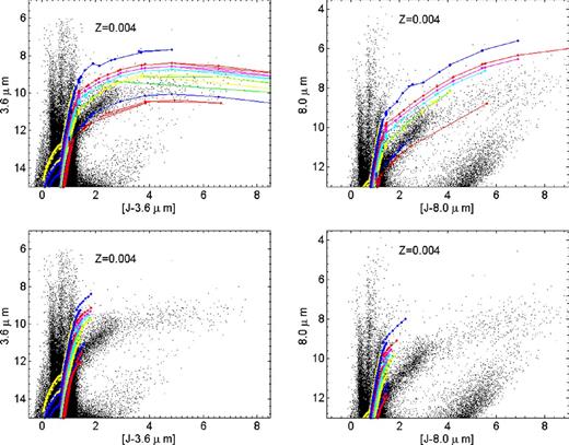
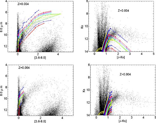
9.1.2 Discussion of field star CMDs
All CMDs of LMC and SMC field stars show the clear effect of dusty circumstellar shells around AGB stars on NIR and MIR colours. Without dust, the theoretical colours are not able to reproduce the observed AGB populations. In fact, without dust the AGB phase does not extend towards very red colours, as observed.
In general, isochrones of the appropriate age reproduce the observed AGB sequences, even though in some cases we do not have an exact match. The reason is the too-coarse grid of ages we are using. Nevertheless, the fit of the observed CMDs with synthetic CMDs generated with population synthesis techniques is beyond the aims of this study. For our purposes, it is enough to test whether the new isochrones (and SSPs) can cover the observed colour range of AGB stars. By inspecting the various CMDs we draw the following conclusions.
At very low ages (log t = 7.95; the yellow line in the online article in the upper left corner of the CMDs, clearly visible in all CMDs except for Figs 19 and 21), AGB stars are not present. The most prominent NIR emitters are red supergiant stars.
In the age range 8.10 ≤ log t ≤ 8.90, the TP-AGB phase is well developed. This is the age range in which AGB models best reproduce the red tail of carbon-rich stars. For these metallicities, intermediate-mass stars develop an extended carbon-rich envelope during the AGB phase. The duration of the carbon-rich phase is determined by the interplay between dredge-up and mass loss. As already pointed out, the efficiency of the TDU increases with decreasing metallicity; it is very efficient for the compositions we are considering.
For ages in the range 9.18 ≤ log t ≤ 9.30, the TP-AGB phase becomes shorter: the carbon-rich envelope is less important, even if its contribution to the red tail is still relevant.
The agreement between our new models and observations is satisfactory for most of the CMDs and is a significant step forward towards a more realistic description of AGB stars. Similar results have been obtained by Marigo et al. (2008) using synthetic TP-AGB models and a library of dusty spectra of AGB stars. We may also observe that our isochrones, thanks to the new libraries of spectra for M and C stars, have a more regular behaviour in the CMDs compared with those of Marigo et al. (2008). This is likely due to the different optical depths adopted for the models (in particular, different recipes for the mass-loss rate).
Only in the 2MASS [Ks]versus [J − Ks] CMDs did the models not match the data satisfactorily. Our AGB isochrones bend towards fainter Ks magnitudes and redder [J − Ks] colours more than the observations, which would suggest a nearly constant Ks. It is hard to trace back the reasons for the discrepancy, considering that in all other NIR/MIR bands the agreement is very good. It could be due to some unrealistic absorption effect in the Ks band. Work is in progress to clarify this issue.
9.2 Integrated colours of star clusters and SSPs
We now compare our models with integrated photometry of star clusters. Figs 22 and 23 show the time evolution of theoretical [V − Ks] and [J − Ks] colours for SSPs with and without the contribution of dusty shells. They are superimposed on optical and near-infrared colours of LMC star clusters, taken from the data base by Pessev et al. (2006, 2008).
![Upper panel: theoretical [V − Ks] colours of our SSPs, with (solid lines) and without (dashed lines) the contribution of circumstellar dust shells around AGB stars, as a function of age (from 0.01 to 15 Gyr, with t in yr). We considered metallicities Z = 0.004 (blue lines in the online article), Z = 0.008 (magenta lines in the online article) and Z = 0.02 (green lines in the online article). The SSPs are superimposed on the integrated colours of LMC star clusters, taken from the compilation by Pessev et al. (2006, 2008); the data are plotted in different colours according to the cluster age, as labelled. Lower panel: as in the upper panel, but we superimposed SSPs of metallicity Z = 0.0001 (black lines) and Z = 0.0004 (magenta lines).](https://oup.silverchair-cdn.com/oup/backfile/Content_public/Journal/mnras/436/3/10.1093_mnras_stt1778/2/m_stt1778fig22.jpeg?Expires=1716402345&Signature=tCT2YOj8DCqPLvvQIJy~~pyGhlO8h5~BphprM9UfMyT2Z8Bl5g9VA-YzpS4N5jP17zFmnca-qqBZpDQijm9IyTRuM4K1zYo03HYkkqXvzVJdrx34fo71luzVC5XjOsx18hkw~NjT8pmzC~joAb~iqdk708VzO-Snp3y5aBr5WSTurgIJHErKrYlSl2M8o1gKJlL7ECOXa9eFThf1r1Hh7OFkyScAY2E9OCKCyYPdEsvsF6crD6ABShcoB3SfcN4~c0xO2u4pYZ08EYEWhduWUY4AOsZRmSBSP3Qatk-IkTCmFKHulHB~57kJYirZeAegVEyUkkFwldoklZ6y7aWUHA__&Key-Pair-Id=APKAIE5G5CRDK6RD3PGA)
Upper panel: theoretical [V − Ks] colours of our SSPs, with (solid lines) and without (dashed lines) the contribution of circumstellar dust shells around AGB stars, as a function of age (from 0.01 to 15 Gyr, with t in yr). We considered metallicities Z = 0.004 (blue lines in the online article), Z = 0.008 (magenta lines in the online article) and Z = 0.02 (green lines in the online article). The SSPs are superimposed on the integrated colours of LMC star clusters, taken from the compilation by Pessev et al. (2006, 2008); the data are plotted in different colours according to the cluster age, as labelled. Lower panel: as in the upper panel, but we superimposed SSPs of metallicity Z = 0.0001 (black lines) and Z = 0.0004 (magenta lines).
![As Fig. 22, but for the [J − K] colour.](https://oup.silverchair-cdn.com/oup/backfile/Content_public/Journal/mnras/436/3/10.1093_mnras_stt1778/2/m_stt1778fig23.jpeg?Expires=1716402345&Signature=FRHoE83HW~btVO14pdOv~C9E~S99C6x3e7h7y9Nr1nsDAyx9VrlrZh-ykaH0PsmBMODB~hVmlL3lmVxR4qN9aGVv5fHSI2MQ1SV8-OSVkVX0dxC3ndsV89TBt4ZbkzoHfzaszKLkSPA26hR7rkW-px792hP0EPtNn-H7olPzg2mdezRvhN~BK-zM~-SPPuSjq8Owvpra7gjpJra4FQpu4-tNTZoIRhW5pRC954rzZaLc7SW7Aut89SbJmiOSaieJwNxufqzn31nBv~2dU0A6PN2IpWmhS20rFobPS5UQXGmfvPvkKUBAXS2vD0vksS9dzOpzZd8NEJrzhX-ZA-krcg__&Key-Pair-Id=APKAIE5G5CRDK6RD3PGA)
Recently Pessev et al. (2006, and references therein) presented integrated NIR magnitudes (J, H, Ks) and colours for a large sample of star clusters in the LMC and SMC, using 2MASS data. These clusters have good estimates of both age and metallicity and can be used as a calibration set for SSP models. Many clusters have ages in the range between 0.3 and 3 Gyr and consequently their integrated properties are heavily affected by AGB stars, which are extremely luminous in the NIR (Pessev et al. 2006). Pessev et al. (2008) combined these data with new photometry for nine additional objects: the whole resulting set forms the largest existing data base of integrated NIR magnitudes and colours of LMC/SMC star clusters. Moreover, the 2MASS data have also been merged with optical photometry from the works of Bica et al. (1996) and van den Bergh (1981). This data set provides very good coverage of the age–metallicity parameter space of LMC/SMC star clusters.
As in similar studies by Elson & Fall (1985a,b, 1988), Chiosi et al. (1986), Chiosi, Bertelli & Bressan (1988), Girardi et al. (1995) and Pessev et al. (2008), we compare theoretical predictions and observed cluster colours as a function of age, to test the models, to single out possible ages where discrepancies appear and to study the evolutionary history of the photometric properties of a star cluster. As pointed out long ago by Chiosi et al. (1986, 1988) and more recently by Pessev et al. (2008), the comparison between theory and observations yields good results only when stochastic effects on the integrated colours are taken into account. The issue is the following: the calculation of integrated properties of SSPs assumes that all stellar evolutionary phases are well sampled. Therefore, a model will match the observations only if the observed integrated magnitudes/colours sample a number of stars large enough. As a consequence, magnitudes/colours of clusters of similar ages and metallicities hosting AGB stars may display a large spread due to the effect of stochastic fluctuations in the number of bright, short-lived AGB stars, caused by the small, finite number of objects populating a real cluster. In other words, the integrated magnitudes/colours of star clusters with a small, stochastically fluctuating number of AGB stars may take a large range of values that can be very different from the value calculated for a fully sampled AGB phase, with the number of stars appropriately scaled according to the AGB lifetime and the cluster total mass, in compliance with the fuel-consumption theorem (Renzini & Buzzoni 1983).
Although the star clusters of the Magellanic Clouds are richer in stars than Galactic open clusters, stochastic effects can still be sizeable. Attempts to compare theory and observations by means of mean values of the integrated colours of clusters grouped into age bins (Noel et al. 2013) may lead to misleading results. Furthermore, the luminosities and effective temperatures of stars during the TP-AGB phase vary significantly, affecting the colours by deviating from the mean, smoothed isochrone discussed in Section 2. This issue will be treated in detail in a forthcoming article of this series (Salaris et al., in preparation).
The temporal variation of the integrated [V − Ks] colours of LMC clusters is presented in Fig. 22. For the sake of clarity, the upper panel contains theoretical colour–age relations for Z = 0.004, 0.008 and 0.02, while the lower panel shows the same but for SSPs with Z = 0.0001 and 0.0004. Solid lines denote the case with dusty AGB stars, while dashed lines display dust-free results. Fig. 23 shows the same comparisons but for the [J − Ks] colour. The data have been selected (and plotted with different colours) according to their metallicity and age, the latter estimated by Pessev et al. (2006, 2008) from the cluster CMDs (see this article for further details). Four age groups are considered. All these clusters have [Fe/H] >−1.71, therefore they can be classified as metal-rich. The data agree reasonably well with the theoretical age–colour relationships, in particular when appropriate metallicities for the clusters of the LMC are taken into account. This is displayed in the top panels of Figs 22 and 23, for both the colours with and without dust around AGB stars, whereby the difference between the two cases starts when the first AGB stars appear. Finally, we call attention to two ‘bumps’ towards redder colours displayed by the theoretical colour–age relationships: the first one occurs at an age of about 0.1 Gyr and is caused by the onset of the AGB phase; the colour becomes redder because of the increased flux in the near-IR passbands. The second ‘bump’ occurs at an age between 1 and 2 Gyr and is likely due to the development of the RGB phase; this is more evident when higher metallicity is taken into account. See Chiosi et al. (1988), Bressan et al. (1994) and Girardi et al. (1995) for a detailed discussion of the subject.
9.3 The colour–colour diagrams
Two-colour diagrams are powerful diagnostics of several photometric properties of star clusters (see Girardi et al. 1995, for a detailed discussion of the issue). Following Piovan et al. (2003), we selected a small sample of clusters, the AGB population of which provides a strong contribution to the integrated light. These photometric data come from the 2MASS Second Incremental Data Release and the Image Atlas, which contains 1.9 million images in the infrared bands J, H and Ks. Pretto (2002) calculated the integrated magnitudes and made them available to us. Moreover, we considered the IR colours for the LMC and SMC clusters by Persson et al. (1983), used by Mouhcine (2002). As for their ages, we rely on the compilation by Pietrzynski & Udalski (2000), who presented age determinations for about 600 star clusters belonging to the central part of the LMC. They are younger than 1.2 Gyr, thus their AGB stars provide a major contribution to the integrated light. Figs 24, 25 and 26 display the two-colour diagrams [H − K] versus [J − H], [H − K] versus [V − K] and [J − K] versus [V − K], respectively. Each diagram shows the data of Persson et al. (1983) for the LMC (open circles) and SMC (black stars) and the data of Pretto (2002) (cross-shaped points), all corrected for reddening. The upper panel of each figure shows the new SSPs with (solid lines) and without (dashed lines) dust shells around AGB stars, whereas the lower panels display the old SSPs by Bertelli et al. (1994). For both types of SSPs, different metallicities are considered, namely Z = 0.02 (magenta lines in the online article), Z = 0.004 (black lines) and Z = 0.008 (green lines in the online article); the age ranges goes from 100 Myr (when AGB stars start contributing to the integrated light of the stellar population) to 13 Gyr, when only low-mass AGB stars are present.
![The two-colour diagram [H − K] versus [J − H] for young star clusters in the Magellanic Clouds. Open circles are LMC clusters selected by Mouhcine (2002) from the catalogue of Persson et al. (1983), while stars (red in the online article) denote the SMC counterpart. Cross-shaped points are LMC clusters, the IR colours of which have been collected by Pretto (2002) using 2MASS data. All data have been reddening-corrected. The lines show the colour range spanned by the new SSPs with (solid lines) and without (dashed lines) the contribution of circumstellar dust shells. Results for different values of the metallicity are shown: Z = 0.02 (magenta in the online article), Z = 0.004 (black) and Z = 0.008 (green in the online article). The range of SSP ages is from 0.1–15 Gyr.](https://oup.silverchair-cdn.com/oup/backfile/Content_public/Journal/mnras/436/3/10.1093_mnras_stt1778/2/m_stt1778fig24.jpeg?Expires=1716402345&Signature=0odagTXPv548KfgcY5r~-Ir6gsChOPrYFFzBbYlb1G7eUJphXfP56LOibZtX8DKu1BRs09ggUtcBFhTZReeJUj1wZa5YHPQi7jnI1cRZjPe5h9ieup4tXiqBYAooRmyF4dTyOvQVjHPdg2H2x5mvMPT7qzfubbgqfV-RBovt6zMyUvsQWlhLJGY~UpjTdsMbLT5i0u~Osk~wea3o70HTQ8zUnHheJBqRXwgnFOclBYxoX~oDFguYn7UnU8spv-ojyvo0pR5QLNPptrXCOEi70DtwbueSmhAHNHj3LKPDH~AK1ye~ZQsVgNiGHYqxtviWJa5O20vvk1AFSJOwXda15A__&Key-Pair-Id=APKAIE5G5CRDK6RD3PGA)
The two-colour diagram [H − K] versus [J − H] for young star clusters in the Magellanic Clouds. Open circles are LMC clusters selected by Mouhcine (2002) from the catalogue of Persson et al. (1983), while stars (red in the online article) denote the SMC counterpart. Cross-shaped points are LMC clusters, the IR colours of which have been collected by Pretto (2002) using 2MASS data. All data have been reddening-corrected. The lines show the colour range spanned by the new SSPs with (solid lines) and without (dashed lines) the contribution of circumstellar dust shells. Results for different values of the metallicity are shown: Z = 0.02 (magenta in the online article), Z = 0.004 (black) and Z = 0.008 (green in the online article). The range of SSP ages is from 0.1–15 Gyr.
![The same as Fig. 24, but for [H − K] versus [V − K] colours. The meaning of the symbols is the same as in Fig. 24.](https://oup.silverchair-cdn.com/oup/backfile/Content_public/Journal/mnras/436/3/10.1093_mnras_stt1778/2/m_stt1778fig25.jpeg?Expires=1716402345&Signature=kQWwVMYwvkJMr3YFvkzgXQ-nJQ66kGBLtNRfGcUjiWWcceYCR146NYDJnTwE6exnfZEsT6~MKn2b20TbC5tjnOXzPjQnNl480MoXyfo7jy7qpzUbvnDMuwimT4TneNM4MMulDRczQg6ThI2eM-i6eoVtO7upgtMiRYN1f81at-xNeega4TI2oCRGT3yP1s3oRR15D9aUwjPzXUf5Fx4qRkdAhUUntFmahcOzyzlfobqW7tseNQlqVmp8Qe5c3b8ZFCgMcDPrm0MyWNj~GdAmjo2MAsNc~WpVP3ESlPsE0yNzNiRq0asp2~KtxShjwlz~e0IK0J2OktRw38zy3ISIAA__&Key-Pair-Id=APKAIE5G5CRDK6RD3PGA)
![The same as Fig. 24, but for [J − K] versus [V − K] colours. The meaning of the symbols is the same as in Fig. 24.](https://oup.silverchair-cdn.com/oup/backfile/Content_public/Journal/mnras/436/3/10.1093_mnras_stt1778/2/m_stt1778fig26.jpeg?Expires=1716402345&Signature=TuQN7TRYfJSZ1MsRb~XROxlrC~-nYIRa9rvh0nmruc5weFan1S-gIEcsLeAhPEo8pShEeMtOTDGwMXR65iM9tlbPXGMJ89ygKnLYL29Kn3ABHsk3qxoMx6IJ53PSKUk6x54jkaePpWF3upUoi1KGa2cRMOKMeYg7wJJUP5bjpxsiBP5GH3Zh9OmpBqKz6Ax71KwOFg4dGxq1qC~Vkk9aOAZA09SLhPB1qTWyGe9lp6zwq2faIEPKazYw0t2nOFGGhZ-0qiN763NXZi7j5dgqScipXRzVP~cW3dD67CtCRBdXYRbeipJL59pz4F2Eei1rBi6RI4w6WRoT~xm9qP4DMQ__&Key-Pair-Id=APKAIE5G5CRDK6RD3PGA)
The new dusty SSPs cover the observed colour ranges better than both the old SSPs by Bertelli et al. (1994) (see Piovan et al. 2003, for more details) and the new ones without dust shells around AGB stars. The dust-free SSPs span a narrower range in [H − K], while the new dusty SSPs extend over a larger [H − K] interval and to bluer [J − H] and [V − K] colours. We recall that the [V − K] colour is particularly suited to studying the AGB phase of stellar populations. In fact, the AGB phase contributes greatly to the NIR light of SSPs between ∼100 Myr and ∼1 Gyr and causes abrupt changes in the NIR luminosity while producing only small changes in the optical. Our new SSPs extend towards bluer colours, approximately like the SSPs by Mouhcine (2002), as shown in Piovan et al. (2003). Differences between our SSPs and the models by Mouhcine (2002) are due to their adoption of empirical spectra for O and C stars, which are limited to the objects they observed and do not cover the full range of relevant parameters (age, metallicity and [C/O] ratio). In our work we instead use theoretical spectra of M stars, which cover all relevant parameter ranges but of course cannot match perfectly the empirical spectra. More work is required to improve the theoretical spectra of cool stars to be included in population synthesis studies.
It is interesting to compare colours that help to break the age–metallicity degeneracy. Following Pessev et al. (2008), we consider the [B − J] versus [J − K] diagram. Puzia, Mobasher & Goudfrooij (2007) have shown that the colour [B − J] is well suited for age estimates, while [J − K] is more sensitive to metallicity (except for the small age interval around the onset of the AGB phase, where [J − K] can show a weak age dependence). We again use the data base by Pessev et al. (2006, 2008), considering the whole metallicity grid and ages from 10–13 Gyr from our new dusty SSPs. Data and theoretical predictions are compared in Fig. 27. The age increases from left to right along the theoretical sequences. We consider here LMC and SMC clusters of any age, split into two groups: young (t < 0.95 Gyr) and old (age above this limit). Furthermore, we subdivide the clusters into metal-rich ([Fe/H] >−1.71) and metal-poor ([Fe/H] above this limit).
![[B − J] versus [J − K] diagrams for a sample of LMC (upper panel) and SMC (lower panel) star clusters. Three combinations of age and metallicity are considered: open circles (red in the online article) denote young (t < 0.95 Gyr) and metal-rich ([Fe/H] >−1.71) clusters, stars (red in the online article) denote old and metal-rich ones and black stars display old and metal-poor objects. Superimposed on the data, we show the new SSPs for different values of metallicity, as labelled.](https://oup.silverchair-cdn.com/oup/backfile/Content_public/Journal/mnras/436/3/10.1093_mnras_stt1778/2/m_stt1778fig27.jpeg?Expires=1716402345&Signature=SkL1Jw58OzIZ7zzUHfP94bKg0KpB1o~grgSDdylbsOAftkiBAgvc3vahg4q8OZXibZpGBvzVH429h8NlJ92S50BmKlonWFOm4~C0caBE9eJOw7Dyq8-aK1QkRPLl099nHJkolJuNCOx0HsRTeiS9g-L9btloUUg6OyY~mpr4SxRaDoG4tq3ZkBUQgpH6uN0msWU7OsN5NF9DRZxfe09KrvhQbNv4v~2CQG1YoojeyiyvaAnIaeSGkqwqgUR~Esoj0ptbFYB2m4nQ0v~JcPLyvINDyr31t7ALdWqAmAfmG4mHATdMi4YDseRIHRrWS53QKbKBO3H3Qf~Vwzy5xIz9gQ__&Key-Pair-Id=APKAIE5G5CRDK6RD3PGA)
[B − J] versus [J − K] diagrams for a sample of LMC (upper panel) and SMC (lower panel) star clusters. Three combinations of age and metallicity are considered: open circles (red in the online article) denote young (t < 0.95 Gyr) and metal-rich ([Fe/H] >−1.71) clusters, stars (red in the online article) denote old and metal-rich ones and black stars display old and metal-poor objects. Superimposed on the data, we show the new SSPs for different values of metallicity, as labelled.
The open circles (red in the online article) denote young and metal-rich clusters, stars (red in the online article) display old and metal-rich ones and, finally, black stars denote old and metal-poor objects. The upper panel shows LMC clusters and the bottom panel SMC ones. In the case of the LMC, we have clusters with all combinations of age and metallicity (only young metal-poor clusters are lacking), while for the SMC the data base does not include any metal-poor objects. There is a clear separation between the different age and metallicity groups: our theoretical colours overlap with the data, particularly in the region of the youngest metal-rich clusters. In contrast, they fail to match the old clusters of the LMC between 0.3 ≲ [B − J] ≲ 0.6 and 2 ≲ [J − K] ≲ 5, which are mostly old and metal-poor (even if some metal-rich clusters appear in this region). We also encountered some problems in the region between 1 ≲ [B − J] ≲ 1.3 and 2 ≲ [J − K] ≲ 3, populated by the oldest metal-rich clusters. Of course, this partial disagreement with observations suggests that some of the ingredients of the models should be improved, like the spectra for the cool stars in our stellar spectra library. It is, however, important to notice, as already pointed out, that stochastic fluctuations of the number of giant stars will always cause a spread of cluster colours at any age and metallicity. This effect is obviously amplified in the case of SMC clusters, considering that we are analysing only a very small number of objects. Stochastic fluctuations could explain the disagreement between data and theory in the above colour intervals as well.
9.4 Clusters of M31
Before concluding, we examine a sample of star clusters in M31, another Local Group galaxy, with a distance modulus of 24.47 mag (Holland 1998; Stanek & Garnavich 1998; McConnachie et al. 2005). M31 is the ideal Local Group galaxy to study globular clusters, since it contains more globulars than all other Local Group galaxies combined (Battistini et al. 1987; Harris 1991; Racine 1991; Fusi Pecci et al. 1993). The globular cluster system of M31 has been extensively studied over many decades (see Ma 2012, for a recent review of the subject). In the following we focus on clusters located in the outskirts of this galaxy, because they are useful probes of the substructures expected to form in the outer region of the host galaxy (Ma 2012), as predicted by the popular ΛCDM model for galaxy formation. This model predicts that these substructures continue to grow in time, from accretion and the disruption of companion satellites.
We make use of the JH, and Ks magnitudes from 2MASS imaging of 10 globular clusters in the outermost regions of M31, analysed by Ma (2012). These data have been combined with V and I photometry (Galleti et al. 2004, 2006, 2007; Huxor et al. 2008). The sample of M31 halo globular clusters is taken from Mackey et al. (2006, 2007), who evaluated the metallicities (−2.14 < [Fe/H] < −0.70), distance modulus and reddening from their CMDs, using deep images obtained with the Advanced Camera for Surveys (ACS) on the HST. The cluster ages have been determined by Ma (2012), by comparing the integrated photometry with the SSP models by Bruzual & Charlot (2003), based upon the Fagotto et al. (1994a,b,c) evolutionary tracks and a Salpeter IMF from 0.1 Mȯ to 100 Mȯ. We adopt these age determinations, the same [V − I] and [J − K] colours and associated uncertainties, and compare these data with our SSPs with circumstellar dust around AGB stars. The upper panel of Fig. 28 displays the theoretical evolution of [V − I] as a function of age, whereas the bottom panel does the same for [J − K] colour. The [V − I] colour appears best suited to match the age and metallicity of these clusters. Moreover, the uncertainties associated with the observational data are lower for this colour compared with [J − K]. As a last remark, we note that for some clusters Ma (2012) assigned a very high age, not only beyond the upper limit of our SSPs (this is not a problem because they can be easily extended) but more importantly well beyond the limit set by Wilkinson Microwave Anisotropy Probe (WMAP-5) data on the age of the Universe, e.g. 13.772 ± 0.059 Gyr (Dunkley et al. 2009).
![Theoretical evolution of [V − I] (upper) and [J − K] (lower) colours as a function of age. SSPs for different metallicities are shown, as labelled. The time t is in yr. The data and their uncertainties are from Ma (2012).](https://oup.silverchair-cdn.com/oup/backfile/Content_public/Journal/mnras/436/3/10.1093_mnras_stt1778/2/m_stt1778fig28.jpeg?Expires=1716402345&Signature=sGKkiBEmbjtS2CJ72wl4n4XAS-Vwk5TVxKpXNr2r6y-gnXqEDEyu3G2bBD4CkxrR2thiqEZWR808CiwsJ8JaXi~S93WHeKlNxLwyBFWqcYrU23AhXL7s8iANi~J52qmEnTsvGH-SPXwG8iCDEgeB2bp6srpawEJU~DzjfdkGMy69Rk1K2s8XY8WEhXJBAMiEoyxul3JEDUSaOAzl5aG5pZeSMSEp1IiFhMfKzMu83dDNEzf-EX-TUPvA6M9CqD0gPyTRmVaPsHoEv2r2w51KWRbDF4o7YwfGFZnb7agvd0Kp81SSEu9jZaD1fAPoQpUvedN9OanTNdqPeJYgE~xMSA__&Key-Pair-Id=APKAIE5G5CRDK6RD3PGA)
Theoretical evolution of [V − I] (upper) and [J − K] (lower) colours as a function of age. SSPs for different metallicities are shown, as labelled. The time t is in yr. The data and their uncertainties are from Ma (2012).
10 SUMMARY AND CONCLUSIONS
Using state-of-the-art AGB models of low- and intermediate-mass stars and accounting for the effect on the model SED of dust shells surrounding the AGB central star, we have revised the Padua library of isochrones (Bertelli et al. 1994) to cover a wide range of chemical compositions (using a helium to heavy-element enrichment ratio ΔY/ΔZ = 2.5) and ages.
The TP-AGB phase is taken from the detailed full evolutionary calculations by Weiss & Ferguson (2009). Two spectral libraries, containing about 600 dust-enshrouded SEDs of AGB stars each, have been calculated, one for oxygen-rich M stars and one for carbon-rich C stars. Each library considers different values of the necessary input parameters (like the optical depth τ, dust composition and temperature at the inner boundary of the dust shell). This is one of the few theoretical studies of stellar SEDs with dusty AGB stars, suitable for use in EPS models. The AGB star SEDs have been implemented into larger libraries of theoretical stellar spectra, to cover all relevant regions of the HRD where stars with a large range of initial stellar mass and chemical composition are found.
Starting from these isochrones and SEDs, we have calculated the integrated SEDs, magnitudes and colours of SSPs with several different metallicities (six values) and ages (more than 50 values from to ∼3 Myr to 15 Gyr) and nine choices of the IMF.
The new isochrones and SSPs have been compared with CMDs of stellar populations in the LMC and SMC, with particular emphasis on the match to the observed AGB sequences. We also compared our theoretical predictions with integrated colours of star clusters in the same galaxies, using data from the SAGE catalogues (Blum et al. 2006; Bolatto et al. 2007), which match IRAC (or MIPS) data with 2MASS photometry. Finally, we have examined the integrated colours of star clusters located on the outskirts of M31.
The agreement between theory and observations is generally good, even if some discrepancies still occur. In particular, the new SSPs reproduce the very extended red tails of AGB stars in CMDs.
The entire libraries of spectra, isochrones and SSPs are made freely available to the scientific community and can be obtained from the authors upon request.
ACKNOWLEDGMENTS
We would like to thank the anonymous referee whose comments improved the quality of the manuscript. We are deeply grateful to Alberto Buzzoni for fruitful discussions. LPC, LP and MS acknowledge the Max-Planck-Institut für Astrophysik (Garching, Germany) for warm and friendly hospitality and computational support during the visits when part of this study was carried out. LPC is also grateful to P. Marigo for useful discussions and to D. Maccagni and M. d. C. Polletta for their support. This study makes use of data products from 2MASS, which is a joint project of the University of Massachusetts and the Infrared Processing and Analysis Centre/California Institute of Technology, founded by the National Aeronautics and Space Administration and the National Science Foundation.
See http://www.mathworks.it/help/techdoc/index.html for MATLAB documentation and more details.
