


Abstract
Upon its completion, the Herschel Astrophysics Terahertz Large Area Survey (H-ATLAS) will be the largest sub-millimetre survey to date, detecting close to half-a-million sources. It will only be possible to measure spectroscopic redshifts for a small fraction of these sources. However, if the rest-frame spectral energy distribution (SED) of a typical H-ATLAS source is known, this SED and the observed Herschel fluxes can be used to estimate the redshifts of the H-ATLAS sources without spectroscopic redshifts. In this paper, we use a sub-set of 40 H-ATLAS sources with previously measured redshifts in the range 0.5 < z < 4.2 to derive a suitable average template for high-redshift H-ATLAS sources. We find that a template with two dust components (Tc = 23.9 K, Th = 46.9 K and ratio of mass of cold dust to mass of warm dust of 30.1) provides a good fit to the rest-frame fluxes of the sources in our calibration sample. We use a jackknife technique to estimate the accuracy of the redshifts estimated with this template, finding a root mean square of Δz/(1 + z) = 0.26. For sources for which there is prior information that they lie at z > 1, we estimate that the rms of Δz/(1 + z) = 0.12. We have used this template to estimate the redshift distribution for the sources detected in the H-ATLAS equatorial fields, finding a bimodal distribution with a mean redshift of 1.2, 1.9 and 2.5 for 250, 350 and 500 μm selected sources, respectively.
1 INTRODUCTION
Much of the optical emission from distant galaxies is absorbed by dust and re-radiated at sub-millimeter (sub-mm) wavelengths (Fixsen et al. 1998). Sub-mm observations have revealed a population of dusty galaxies at z > 2, previously hidden at optical wavelengths (see review by Blain et al. 2002). The inferred star formation rates for these galaxies are huge, averaging at ≃400 M⊙ yr−1 (Coppin et al. 2008). Observations of sub-mm galaxies (SMGs) allow us to examine star formation in the early universe and the strong cosmic evolution in the star formation rate (Gispert, Lagache & Puget 2000). Ground-based surveys have managed to identify and study individual sub-mm sources (Barger et al. 1998; Hughes et al. 1998; Blain et al. 1999). Such surveys however covered small areas of sky and only found a few tens of SMGs and suffered from biases in their selections. The Balloon-born Large Aperture Submillimeter Telescope (BLAST) survey (Devlin et al. 2009) covered ∼9 deg2 of sky and found a few hundred SMGs (Eales et al. 2009) but to really probe the evolution of the SMGs with redshift much larger blind surveys are needed.
In order to investigate the SMGs, particularly the evolution of the star formation rate and the luminosity function, we need to know the redshifts of all sources being considered. Ideally, this is done by matching a source to an optical counterpart and then measuring the redshift of this counterpart spectroscopically. However, the poor angular resolution of sub-mm telescopes and high confusion between sources mean that finding optical counterparts in this way is difficult. One method to find counterparts is to first match the sub-mm source to a mid-infrared (mid-IR) or radio source, then match the mid-IR/radio source to its corresponding optical counterpart. This can lead to a bias; however, as cold or high-redshift objects are more likely to be undetected at mid-IR and radio wavelengths (Chapman et al. 2005; Younger et al. 2007).
Fully exploiting the potential of sub-mm wavelengths on a large scale was impossible until the advent of the Herschel Space Observatory (Pilbratt et al. 2010).1 The infrared emission of galaxies peaks between |$70\text{ and }500\,\mu$|m, the wavebands that are covered by Herschel's two instruments: the Spectral and Photometric Imaging Receiver (SPIRE; Griffin et al. 2010) and the Photodetector Array Camera and Spectrometer (PACS; Poglitsch et al. 2010). The Herschel Astrophysics Terahertz Large Area Survey (H-ATLAS; Eales et al. 2010)2 covers 550 deg2 of sky and is the largest sub-mm blind survey to date.
The H-ATLAS fields were chosen partly due to the high quantity of complementary data at other wavelengths. However, less than 10 per cent of the H-ATLAS sources in the 15 h field are detected by WISE at 22 μm (Bond et al. 2012) and current large-area radio surveys only detect a tiny fraction of H-ATLAS sources. Nevertheless, Smith et al. (2011) and Fleuren et al. (2012) have shown that it is possible, using a sophisticated Baysian technique, to match the H-ATLAS sources to optically detected galaxies directly. However, only approximately a third of the H-ATLAS sources have single reliable optical counterparts on images from the Sloan Digital Sky Survey (SDSS) (Smith et al. 2011) which has limited subsequent investigations into the luminosity (Dye et al. 2010) or dust mass (Dunne et al. 2011) functions. Matching to the near-infrared images from the VISTA Infrared Kilo-degree Infrared Galaxy (VIKING) survey produces a higher proportion of counterparts, 51 per cent opposed to the 36 per cent provided by the optical (Fleuren et al. 2012), but there are still a large number of sources without counterparts.
CO line spectroscopy, using wide band instruments, can be used to accurately measure the redshift of sub-mm sources without the need for accurate optical positions (Frayer et al. 2011; Harris et al. 2012; Lupu et al. 2012). However, CO observations are time consuming and even with Atacama Large Millimeter Array it will only be possible to measure redshifts for a tiny fraction of the H-ATLAS sources.
The only feasible method currently for estimating redshifts for such a large number of Herschel sources is to estimate the redshifts from the sub-mm fluxes themselves. Previous attempts to estimate redshifts for Herschel sources from the sub-mm fluxes have used as templates the spectral energy distributions (SEDs) of individual galaxies e.g. Lapi et al. (2011); González-Nuevo et al. (2012). Many of these template galaxies are at low redshift and their SEDs may not be representative of the SEDs of the high-redshift Herschel sources and even if a high-redshift galaxy is used it may not be representative of the high-redshift population as a whole. For these reasons, we describe in this paper a method for creating a template directly from the sub-mm fluxes of all the high-z H-ATLAS sources for which there are spectroscopic redshifts. The SEDs are also important for increasing our understanding of the population of high-redshift dusty galaxies and investigating the SEDs at the range of wavelengths in which the dust emission is at its peak. The average SED that we derive in this paper, although obviously telling us nothing about the diversity of the population, is still useful for comparing this population with dusty galaxies of low redshift (Dunne & Eales 2001; Blain, Barnard & Chapman 2003).
Section 2 describes the observations on which the method is based. We describe the method of template determination in Section 3 and present the estimated redshift distributions in Section 4. We summarize our results in Section 5. We assume Ωm = 0.3, Ωλ = 0.7, H0 = 70 km s−1 Mpc−1.
2 DATA
2.1 Far-infrared (FIR) images and catalogues
Phase 1 of the H-ATLAS survey covers around 160 deg2 of sky with both PACS observations at 100 and 160 μm and SPIRE observations at 250, 350 and 500 μm. However, only a few per cent of the H-ATLAS sources were detected at PACS wavelengths at greater than 5σ, so we have developed a method of estimating redshifts using only the SPIRE fluxes. Phase 1 coincides with the three equatorial fields of the Galaxy and Mass Assembly (GAMA; Driver et al. 2011) spectroscopic survey.
The full width at half-maximum beam sizes of the SPIRE observations are 18, 25 and 35 arcsec for 250, 350 and 500 μm, respectively. Pascale et al. (2011) describes the map-making procedure for the SPIRE observations. To find the sources, the madx algorithm (Maddox et al. 2010; Rigby et al. 2011) was used on the maps that had been passed through a point spread function filter. The algorithm initially used the 250 μm map to find the positions of sources detected above 2.5σ. The corresponding fluxes from the 350 and 500 μm maps were then measured at these positions. If a source was detected at greater than 5σ in any of the three wavebands then it was listed as a detection, with 78 014 sources extracted in total. The 5σ sensitivities of the catalogues are 32, 36 and 45 mJy for 250, 350 and 500 μm, respectively. The error on the flux, σmeas, is the combined instrumental and confusion noise with an additional 7 per cent calibration error added in quadrature. The Phase 1 Herschel maps and catalogues will be described fully in Valiante (in preparation).
2.2 Optical counterparts
The fields were chosen due to their lack of galactic cirrus (though G09 does still contain a large amount of cirrus) and large amount of complementary multiwavelength data. However, the lack of radio and mid-IR data meant counterparts were found directly by applying a likelihood ratio technique (Smith et al. 2011) to objects in the SDSS (York et al. 2000) DR7 catalogue with a search radius of 10 arcsec. Only optical objects matched with a reliability factor of R ≥ 80 per cent were considered as reliable matches.
23 312 sources have reliable optical counterparts. For these there is photometry in ugriz and YJHK from the SDSS and UKIRT Infrared Deep Sky Survey Large Area Survey (Lawrence et al. 2007), respectively, and far-ultraviolet and near-ultraviolet data from Galaxy Evolution Explorer (GALEX) (Martin et al. 2005). 12 136 sources also have spectroscopic redshifts available from the SDSS, 6DF Galaxy Survey (Jones et al. 2009) and 2SLAQ-QSO/LRG (Cannon et al. 2006; Croom et al. 2009) surveys and from the GAMA catalogues (Driver et al. 2011). A further 10 972 photometric redshifts have been estimated from optical and near-IR photometry using the artificial neural network code (annz) (Smith et al. 2011). These redshift distributions are shown in Fig. 1. In Fig. 2, sources without optical counterparts are shown to have slightly redder sub-mm colours, suggesting that they lie at higher redshifts than those with counterparts.
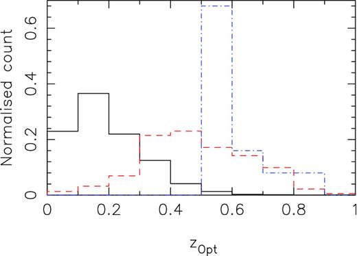
Redshift distributions of the H-ATLAS galaxies as determined from their SDSS counterparts. The solid black line shows those with measured spectroscopic redshifts and the dashed red line those with photometrically estimated redshifts only. The dot–dashed blue line shows the redshift distribution of the objects in the sample used to derive the template (Section 3): 25 spectroscopically observed sources with 0.5 < z < 1.0 and S250 > 50 mJy.
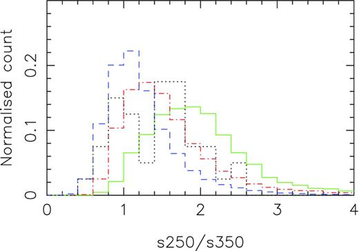
Histograms of the ratio of 250 to 350 μm fluxes. The solid green line represents those with spectroscopically measured optical counterparts. The dot–dashed red line shows sources with only photometric redshifts. The blue dashed line shows sources without any optical counterpart. The black dotted line shows the sample of 40 sources in the sample used to derive the template (Section 3). Sources without counterparts are redder in colour, indicating a higher redshift population.
2.3 CO observations
We used 15 H-ATLAS sources with redshifts from CO observations to construct our template. These sources are listed in Table 1. Five of these are from Lupu et al. (2012), who measured CO redshifts for sources with S500 > 100 mJy; seven are from Harris et al. (2012), who observed galaxies whose sub-mm emission peaked at 350 μm, indicating a high redshift; one is from Cox et al. (2011), who studied one of the brightest sources in the GAMA 15 h field, which has the peak of its emission at 500 μm; and the remaining two are as yet unpublished redshifts from the H-ATLAS team.
The selection criteria for these follow-up observations picked out bright galaxies that were likely to be at high redshift and so only represent the most luminous high-z galaxies. The Herschel colours of these galaxies are very red, which might introduce a bias towards colder objects. There is also a bias towards galaxies that are rich in CO gas, since not all sources observed in the CO programme were detected. Many of these sources are likely to have been strongly lensed (Negrello et al. 2010; Harris et al. 2012). As the gravitational magnification is likely to vary over a source it is possible that an unusually warm section of a galaxy might be magnified more strongly, boosting the flux at short wavelengths. However, the dust detected at SPIRE wavelengths is likely to be cool and evenly distributed throughout the galaxy and so the Herschel colours are likely to remain reasonably unaffected and resulting temperatures can be taken as safe upper limits.
3 THE TEMPLATE
3.1 Sample selection
To create the template, we formed a sample of bright sources with accurately known redshifts. To do this, we selected sources with either a redshift determined from the CO observations, zCO, or an optically determined redshift, zspec, with 0.5 ≤ zspec < 1. In addition, the flux must be greater than 50 mJy in at least one of the SPIRE wavelengths. Optically selected sources with zspec > 1 are more likely to be quasars or atypical galaxies and so we did not use sources with optically determined redshifts above this reshift. The flux and redshift limits ensure that we have a selection of high-z sources for which we have accurate measurements of the SEDs.
We excluded sources at z < 0.5 for two reasons. First, these sources do not actually provide much extra information about the rest-frame Herschel SEDs, because for low-redshift galaxies the SPIRE colours depend very weakly on dust temperature. Secondly, there is evidence from studies that combine the PACS and SPIRE data for individual sources (Lapi et al. 2011; Smith et al. 2012) and from stacking analyses (Eales in preparation) that the SEDs of low-redshift and high-redshift Herschel sources are quite different.
These selection criteria produced a sample of 40 sources with known redshifts which are given in Table 1: 15 sources with CO redshifts and 25 sources with optical redshifts. There are actually many more sources in the redshift range 0.5 < z < 1.0 with optical redshifts, but 25 were randomly chosen in order to prevent them from overwhelming the CO sources. We assume that this sample is representative of the whole survey; their redshifts and Herschel colours are shown for comparison in Figs 1 and 2. The colours of this sample seem to be similar to those of sources with no optical counterpart. However, a possible bias may arise from the fact that all these sources are chosen to be bright and so will be among the most luminous H-ATLAS sources at their respective redshifts and so may not be representative of less luminous sources (Casey et al. 2012). We will use PACS data to test the dependence of dust temperature on luminosity in a later paper (Eales in preparation).
3.2 Creating the template
A two temperature model is important because galaxies with high FIR luminosities are known to contain a cold dust component (Dunne & Eales 2001). We used β = 2 because recent Herschel observations of nearby galaxies suggest this is a typical value (Eales et al. 2012). The SPIRE fluxes for the H-ATLAS sources do not give useful constraints on β as they do not lie in the Rayleigh–Jeans region of the SED, where β has the greatest effect.
For each combination of Tc, Th and a, we found the values of Ni that gave the minimum value of χ2. Our best-fitting model was the set of Tc, Th and a that gave the lowest value of χ2 overall, resulting in the template shown in Fig. 3 and the values given in Table 2. Our best-fitting model gives Tc = 23.9 K, Th = 46.9 K with a ratio of cold to hot dust mass being 30.1. For comparison, we have also shown the SEDs of SMM J2135−0102 (z = 2.3) and G15.141 (z = 4.2) in Fig. 4, as used in Lapi et al. (2011) for estimating the redshifts of the sources in the H-ATLAS field observed during the Herschel Science Demonstation Phase (SDP). All SEDs are normalized to the best values of Ni given by our template as seen in Fig. 3. The template we find from the sample peaks at a slightly higher wavelength than that of those found in Lapi et al. (2011) though the Rayleigh–Jeans region has very similar slope, most likely as both use β = 2 for at least one of the dust components. When compared to the SED from Casey et al. (2012), generated from spectroscopically selected HerMES galaxies, the peak lies in a very similar position. The SED derived by Casey et al. (2012) is controlled by a power law shortward of the peak to cover the mid-IR component, which is why it is so different from the other SEDs. However, this region is well below the rest-frame wavelength sampled by our SPIRE observations.
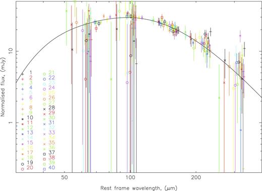
Best-fitting model with the rest-frame fluxes for all 40 of the sources in Table 1, adjusted by their best normalization factors, Ni. The red and blue lines show the SEDs for the individual dust components of our template. All fluxes from a given source are shown with the same plot points, the key of which is given in Table 1.
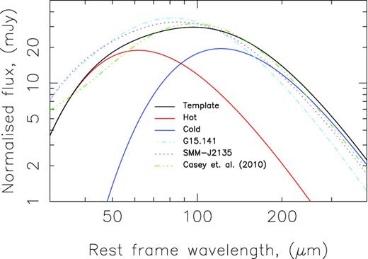
Best-fitting model as compared with the SEDs from G15.141 (dotted magenta) and SMM J2135−0102 (dot–dashed cyan) used by Lapi et al. (2011) and the best-fitting SED from Casey et al. (2012) (green triple-dot–dash). The comparative SEDs have been normalized to best fit the fluxes as they are shown in Fig. 3.
Results of the jackknife tests applied to the data. ‘Template’ indicates the sub-set used to create the template and the temperatures and dust mass ratios of the template are listed in the following three columns. ‘All’ is the template resulting from using the whole sample and is the template that will be used in subsequent sections. The next two columns show our estimates of the redshift errors that will be obtained using that template, which were obtained by comparing the redshift estimates and the spectroscopic redshifts for the sources in the other member of the jackknife pair (or all the sources for the template that was obtained from the whole sample). Column 5 shows the mean value of Δz/(1 + zspec) and column 6 gives the root mean squared (rms) of this. Column 7 gives the key for Fig. 5. The two rows below the line show the result of testing two of the templates used by Lapi et al. (2011) against our calibration sample.
| Template | Tc | Th | a | Δz/(1 + z) | rms | Key |
|---|---|---|---|---|---|---|
| 1 | 24.8 | 45.5 | 22.25 | 0.06 ± 0.04 | 0.28 ± 0.03 | Black |
| 2 | 22.2 | 43.0 | 22.22 | −0.03 ± 0.03 | 0.24 ± 0.03 | Red |
| 3 | 18.8 | 39.6 | 20.97 | −0.06 ± 0.03 | 0.24 ± 0.03 | Green |
| 4 | 26.6 | 51.1 | 44.55 | 0.08 ± 0.04 | 0.29 ± 0.03 | Blue |
| 5 | 22.9 | 44.3 | 24.15 | 0.01 ± 0.03 | 0.25 ± 0.03 | Cyan |
| 6 | 18.3 | 34.3 | 5.41 | 0.02 ± 0.04 | 0.27 ± 0.03 | Magenta |
| All | 23.9 | 46.9 | 30.10 | 0.03 ± 0.04 | 0.26 ± 0.03 | – |
| SMM | – | – | – | 0.135 | 0.332 | – |
| G15.141 | 32.0 | 60.0 | 50.0 | 0.269 | 0.431 | – |
All sources used to make up the template sample. Follow up observations were taken using the Caltech Submillimeter Observatory (CSO) with Z-Spec, IRAM Plateau de Bure Interferometer (PdBI), Green Bank Telescope (GBT) with Zpectrometer, Combined Array for Research in Millimeter-wave Astronomy (CARMA), Atacama Pathfinder Experiment (APEX), Sub Millimeter Array (SMA). All spectroscopic redshifts (those above the line) are from the Sloan Digital Sky Survey (SDSS) Data Release 7 (DR7) (York et al. 2000). CO redshifts are listed after the linebreak where H12 is Harris et al. (2012), F11 is Frayer et al. (2011) and L12 is Lupu et al. (2012).
| No. | H-ATLAS name | z | Reference | Observations |
|---|---|---|---|---|
| 1 | HATLAS J143845.8+013504 | 0.501 | SDSS DR7 | SDSS |
| 2 | HATLAS J140746.5−010629 | 0.507 | SDSS DR7 | SDSS |
| 3 | HATLAS J090758.2−001448 | 0.516 | SDSS DR7 | SDSS |
| 4 | HATLAS J142534.0+023712 | 0.518 | SDSS DR7 | SDSS |
| 5 | HATLAS J143703.8+014128 | 0.522 | SDSS DR7 | SDSS |
| 6 | HATLAS J141815.6+010247 | 0.524 | SDSS DR7 | SDSS |
| 7 | HATLAS J083713.3+000035 | 0.534 | SDSS DR7 | SDSS |
| 8 | HATLAS J090359.6−004555 | 0.538 | SDSS DR7 | SDSS |
| 9 | HATLAS J140640.0−005951 | 0.539 | SDSS DR7 | SDSS |
| 10 | HATLAS J140930.6−013805 | 0.539 | SDSS DR7 | SDSS |
| 11 | HATLAS J141343.4+004041 | 0.546 | SDSS DR7 | SDSS |
| 12 | HATLAS J121353.8−024317 | 0.557 | SDSS DR7 | SDSS |
| 13 | HATLAS J092340.2+005736 | 0.560 | SDSS DR7 | SDSS |
| 14 | HATLAS J120248.3−022944 | 0.563 | SDSS DR7 | SDSS |
| 15 | HATLAS J114619.8−014356 | 0.571 | SDSS DR7 | SDSS |
| 16 | HATLAS J141429.0−000900 | 0.574 | SDSS DR7 | SDSS |
| 17 | HATLAS J085230.1+002844 | 0.584 | SDSS DR7 | SDSS |
| 18 | HATLAS J143858.1−010540 | 0.615 | SDSS DR7 | SDSS |
| 19 | HATLAS J084846.2+022032 | 0.627 | SDSS DR7 | SDSS |
| 20 | HATLAS J120246.0−005221 | 0.653 | SDSS DR7 | SDSS |
| 21 | HATLAS J113859.3−002934 | 0.684 | SDSS DR7 | SDSS |
| 22 | HATLAS J084217.0+010920 | 0.761 | SDSS DR7 | SDSS |
| 23 | HATLAS J090420.9+013038 | 0.792 | SDSS DR7 | SDSS |
| 24 | HATLAS J114023.0−001043 | 0.844 | SDSS DR7 | SDSS |
| 25 | HATLAS J141148.9−011439 | 0.857 | SDSS DR7 | SDSS |
| 26 | HATLAS J142935.3−002836 | 1.026 | ZSpec, CARMA | |
| 27 | HATLAS J090740.0−004200 | 1.577 | L12 | CSO |
| 28 | HATLAS J091043.1−000321 | 1.784 | L12 | CSO |
| 29 | HATLAS J085358.9+015537 | 2.091 | ZSpec, PdBI | |
| 30 | HATLAS J115820.2−013753 | 2.191 | H12 | GBT |
| 31 | HATLAS J090302.9−014127 | 2.308 | L12 | CSO, CARMA, GBT, PdBI |
| 32 | HATLAS J084933.4+021443 | 2.410 | H12 | CARMA, GBT |
| 33 | HATLAS J141351.9−000026 | 2.478 | H12 | GBT |
| 34 | HATLAS J113243.1−005108 | 2.578 | H12 | GBT |
| 35 | HATLAS J091840.8+023047 | 2.581 | H12 | GBT |
| 36 | HATLAS J091305.0−005343 | 2.626 | L12, F11 | CSO, GBT, PdBI |
| 37 | HATLAS J090311.6+003906 | 3.037 | L12, F11, H12 | CSO, PdBI, GBT |
| 38 | HATLAS J113526.3−014605 | 3.128 | H12 | GBT |
| 39 | HATLAS J114637.9−001132 | 3.259 | H12 | GBT |
| 40 | HATLAS J142413.9+022303 | 4.243 | Cox et al. (2011) | APEX, FLASH+, PdBI, SMA |
It should be noted that the template is not expected to be a physically real SED but simply a statistical tool for estimating redshifts from SPIRE fluxes. The peak of Fig. 3 will represent the real SED of sources with z ∼ 2–4, with the SED at longer wavelengths representing the real SED of H-ATLAS galaxies at lower redshift. In a later paper, we will make a more detailed comparison of the SEDs of high-redshift H-ATLAS galaxies with low-redshift dusty galaxies. Here, we note that the average SED is quite similar to the two-temperature SEDs found by Dunne & Eales (2001) for luminous low-redshift dusty galaxies.
3.3 A jackknife method for testing the template
In order to test the accuracy of the redshifts determined from the template we used a jackknife technique. From the initial selection of 40 sources we created two sub-sets by listing the sources by redshift and alternately placing them into each sub-set. This ensured an even spread of redshifts and thus equal wavelength coverage. This was repeated twice more, this time splitting the sources randomly, resulting in three pairs of sub-sets from the initial data sample. For each sub-set, we created a template as detailed in Section 3.2. We then used the template to estimate the redshifts, ztemp, of the sources in the other sample from the pair. In estimating the redshifts, the template was allowed to vary in redshift between 0 ≤ z < 20 with the minimum χ2 between the fluxes and the template giving the best estimate of ztemp.
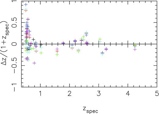
The data was split three ways into pairs of sub-sets. Each of these were used to create a template, then the template used to estimate the redshifts of the other sub-set in the pair. The resulting redshift errors are shown here plotted against the spectroscopic redshifts. The key is given in Table 2.
As our estimate of the uncertainty in the redshifts estimates ztemp from the template obtained from the whole sample, we use the average from all the jackknife tests in Table 2 giving a mean rms of Δz/(1 + z) = 0.26. Note that if we only look at sources where zspec > 1 then the error is much less. Fig. 5 clearly shows that there is much higher accuracy above this cut-off. If we restrict our error analysis to the sources in the template sample with zspec > 1, we obtain a mean Δz/(1 + z) = −0.013 with and rms of 0.12.
Our results are comparable to the error estimates given by Lapi et al. (2011). When the templates from Lapi et al. (2011) (SMM J2135−0102 and G15.141) are used to estimate redshifts for our 40-source sample, there is a larger systematic error than when we use our own template, with the predicted redshifts considerably higher than the actual values. The reason for this can be seen in Fig. 3, which shows that the templates for SMM and G15.141 peak at lower wavelengths compared to our template.
For the subsequent sections, we will use the template created when all sources in the sample were used (‘All’ in Table 2). We have obtained this template from bright sources, whereas the majority of the Phase 1 sources have considerably lower signal-to-noise ratios, increasing the uncertainty in our redshift estimates. To gauge the total effect of this uncertainty on any particular redshift estimate, we have used the template to estimate the redshifts for all the sources in the Phase 1 catalogue. We have then plotted the estimated redshifts against the statistical error, which has been obtained by changing the redshift estimate until there is a change in χ2(Δχ2) of one (one ‘interesting’ parameter, Avni 1976) (Fig. 6). This change in χ2 corresponds to a confidence region of 68 per cent. We can see that the uncertainty on z grows with redshift up to z = 2, where it begins to fall again.
The figure suggests that for a source that is detected at the signal-to-noise limit of the catalogue, the error is about 0.8 if the source is at a redshift of 3 but only 0.08 at a redshift of zero. This, however, ignores the important systematic error caused by the difference in dust temperature between low- and high-redshift H-ATLAS sources, which we address in the next section.
3.4 Cold sources at low redshift
Fig. 6 shows that the statistical error, zerr, for a redshift estimate for a low-redshift source is fairly small, but in reality there is a large systematic effect caused by the fact that low-redshift Herschel sources have much cooler SEDs than the template we have derived from our high-redshift (z > 0.5) spectroscopic sample. This is shown dramatically in Fig. 7, where we have plotted Δz/(1 + zspec) for all H-ATLAS sources with either CO redshifts or optical counterparts (reliability >0.8) and spectroscopic redshifts. As expected, at z > 0.5 the errors are quite small, but of the thousands of sources at z < 0.5 there are a large number with extremely large redshift discrepancies. As we demonstrate below, this is likely to be mostly caused by a systematic temperature difference between low- and high-zHerschel sources, but there will be some discrepancies due to gravitational lensing, in which the Herschel source is really at a very high redshift with the apparent optical counterpart at much lower redshift being the gravitational lens (Negrello et al. 2010; González-Nuevo et al. 2012). The effect of this will be investigated in a subsequent paper.
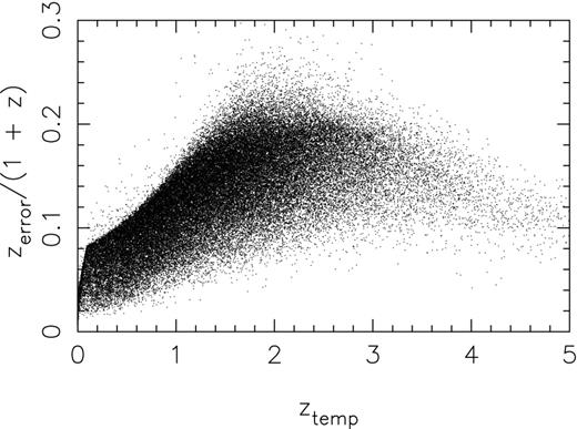
Plot of redshift according to our template against the estimated error as predicted from the χ2 corresponding to a confidence region of 68 per cent (see the text). The hard edge at low ztemp arises as these sources lie on the Rayleigh–Jeans tail and are at the flux limit of the survey.
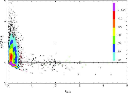
Plot of zspec against Δz/(1 + z) for all sources with measured redshifts, either CO redshifts or optical spectroscopy. Sources with zspec > 1 are shown with crosses for clarity. The contours are included to show the density of sources at low redshifts. The key shows the number of sources in a bin where Δz = 0.04 and Δ(Δz/(1 + z)) = 0.1. The sources in red are the sources with optical redshifts that were used to create the template and the sources in green are the ones with CO measurements.
We have investigated the possibility of systematic errors caused by temperature differences by using a Monte Carlo simulation. In this simulation, we start with the Phase 1 H-ATLAS sources with reliable optical counterparts (reliability >0.8) and redshifts, either spectroscopic or estimates from optical photometry, <0.4. We then use these sources to generate probability distributions for the redshifts and the 250 μm fluxes. The first step in the simulation is to create an artificial sample of galaxies by randomly drawing 250 μm fluxes and redshifts from these distributions. To produce an SED for each galaxy, we randomly assign one of the five average SEDs for low-redshift H-ATLAS galaxies from Smith et al. (2012). This library of SEDs seems the most appropriate for generating an artificial H-ATLAS sample, although we have also used 74 SEDs found for Virgo galaxies by Davies et al. (2012) and the 11 SEDs found for the Key Insights on Nearby Galaxies: a Far-Infrared Survey with Herschel sample by Galametz et al. (2012), with very similar results. We use the SEDs and the redshifts to calculate 350 and 500 μm fluxes for each galaxy. The next step is to add noise to each galaxy. In order to allow for both instrumental noise and confusion, we add noise to each galaxy by randomly selecting positions on the real SPIRE images. We use the SPIRE images that have been convolved with the point spread function, since these were the ones used to find the sources and measure their fluxes. The final step in the simulation is to estimate the redshifts of the sources using our template.
Fig. 8 shows that the systematic errors can be very large. Although ≃80 per cent of the sources have estimated redshifts <1, a significant fraction have higher estimated redshifts, although by z > 2 the number of cool low-redshift sources that are spuriously placed at high redshift is very small. The simulation shows very clearly that one should not rely on this technique for estimating the redshifts of individual sources close to the flux limit of the survey. However, as we show in the next section, we can with care use it to draw some statistical conclusions about the survey.
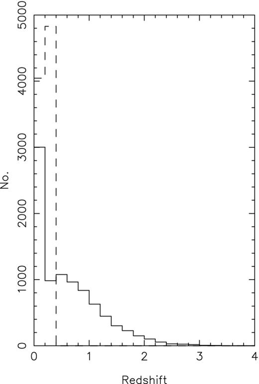
Results of Monte Carlo simulation of our redshift estimation method for sources at low redshift, which are known to have cooler SEDs than our template. The dashed line shows the redshift distribution for sources in the Phase 1 catalogue with reliable identifications which have redshifts (spectroscopic or photometric) <0.4. The solid line shows the redshift distribution for these sources estimated using our template.
4 REDSHIFT DISTRIBUTION
We used the following procedure to estimate the redshift distribution of the H-ATLAS sources. The template was used to estimate the redshifts, ztemp, of all the H-ATLAS Phase 1 sources without an optical counterpart, but where a reliable optical counterpart with a redshift was available we continued to use this value because of the problem described in the previous section. Fig. 9 shows the redshift distributions for sources with fluxes greater than 5σ in a given band. The mean redshift increases with wavelength: z = 1.2, 1.9 and 2.6 for 250, 350 and 500 μm, respectively, due to the increasingly strong K-correction. A high-z tail extends to z ∼ 5 for 350 and 500 μm selection and to z ∼ 4 for 250 μm. *.*
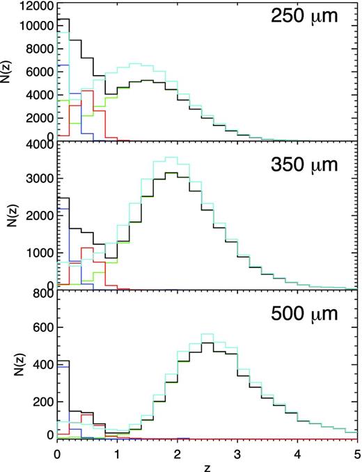
Redshift distribution for sources with fluxes greater than 5σ in the stated waveband. The upper plot shows the 250 μm selection, with a median z = 1.0, the middle 350 μm with a median z = 1.8 and the lower 500 μm with a median z = 2.5. All three show a large number of sources with z < 0.2 and a second broader distribution of sources at much higher redshifts. The dark blue line shows those sources with spectroscopic redshifts from optical counterparts. The red line shows those sources with optical photometric redshifts. The green line shows the redshifts estimated from the template for those sources with no reliable optical counterpart. The black line shows the sum of all three distributions (the median values stated are for these distributions). The light blue line shows the predicted redshift distributions if we do not use the redshifts of the optical counterparts but instead the redshifts estimated using the template.
We see a bimodal distribution with a large number of sources at low-z (z ≤ 0.8), dominated by those sources with optical counterparts. This is seen in all three wavebands, though is most obvious at 250 μm. By requiring that every source must have ztemp ≥ 0, instrumental scatter may increase the size of the low-z peak. However, most of the sources in the low-z peak come from the optical counterparts and few of our estimated redshifts are used, particularly at longer wavelengths. Although, there are undoubtedly H-ATLAS sources at low redshift that do not have reliable counterparts and which may be spuriously placed at high redshift, we do not see any way that this could create the bimodal redshift distribution seen for the 250 μm sample. We have also plotted in the figure the redshift distributions we obtain if we do not use the redshifts of the optical counterparts. At 250 μm, but not at the other two wavelengths, there is still clear evidence of a bimodal distribution. The redshift distribution estimated by Dunlop et al. (2010) for the BLAST survey at 250 μm is quite similar to ours and shows a similar bimodal distribution although it only contains a few tens of sources.
Eales et al. (2010) presented predicted H-ATLAS redshift distributions using models based on the SCUBA Local Universe and Galaxy Survey (SLUGS; Dunne, Clements & Eales 2000) and the model described in Lagache et al. (2004). The results are shown in Fig. 10 alongside our estimated distributions. The SLUGS model predicts few sources with z > 2, in strong disagreement with our results. The Lagache et al. (2004) model predicts a bimodal distribution similar to what we find for the H-ATLAS sources and extends to redshifts similar to our distributions. However, our high-z peaks are at a much higher redshift than predicted by the model.
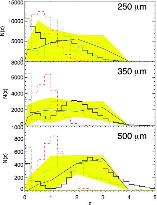
Redshift distribution for sources with fluxes greater than 5σ in the stated waveband. Overlaid are the models from Eales et al. (2010). The model from Lagache et al. (2004) is shown by the green dot–dashed line. The red dashed line is the SLUGS model. The blue triple-dot–dashed line shows the model from Mitchell-Wynne et al. (2012) with 1σ confidence region in yellow. All models have been normalized to the number of sources detected with H-ATLAS.
Lagache et al. (2004) used both normal and starburst galaxies in their model. The differing cosmological evolution of these two populations causes the bimodal distribution seen in the model. Our redshift distribution also shows this bimodality suggesting that there really is two populations of galaxies, although we cannot exclude the possibility that there is a single population, and the effects of the cosmic evolution of this population and the cosmological model combine to produce the bimodal redshift distribution (Blain & Longair 1996). This bimodality provides some support for the conclusions of Lapi et al. (2011) that the high-z H-ATLAS sources represent a different population to the low-z sources: spheroidal galaxies in the process of formation, rather than more normal star-forming galaxies seen at low redshift.
Mitchell-Wynne et al. (2012) created a model by estimating the sub-mm redshift distribution from the strong cross-correlation of Herschel sources with galaxy samples at other wavelengths, for which the redshift distribution is known. The initial redshift distributions were obtained by using 24 μm Spitzer Multiband Imaging Photometer for Spitzer sources to cover the redshift range 0.5 < z < 3.5 and optical SDSS galaxies to cover 0 < z < 0.7. The authors estimate redshift distributions for samples of sources brighter than 20 mJy at the three SPIRE wavelengths, ≃1.5–2 times fainter than the H-ATLAS limits. Their distributions agree quite well with the high-redshift peak of the H-ATLAS sources at all three wavelengths, but their distributions do not show the bimodal distribution that we find.
Amblard et al. (2010) and Lapi et al. (2011) have also estimated redshifts for H-ATLAS sources in the SDP field, which only contained ∼6000 sources. Amblard et al. (2010) used one-temperature modified black bodies with a range of temperature and β to estimate the redshifts for sources from the SDP H-ATLAS field. These sources were selected to be detected at >3σ at 250 and 500 μm and with fluxes greater than 35 mJy (5σ) at 350 μm. These cuts bias against sources at lower redshifts, though the sample still includes several sources that were identified optically.
Amblard et al. (2010) estimated a mean redshift of z = 2.2. In Fig. 11, we have used our template to estimate redshifts for Phase 1 sources that satisfy the same flux criteria as used by Amblard et al. (2010). Unlike Amblard et al. (2010), we find a bimodal distribution, but it is worth noting that the majority of sources in the low-z peak are redshifts from optical counterparts. We find many more sources beyond z > 3. This is presumably due to our use of a two-component dust model rather than the single-component model used by Amblard et al. (2010). We find a mean redshift of 2.0, slightly lower than that found by Amblard et al. (2010).
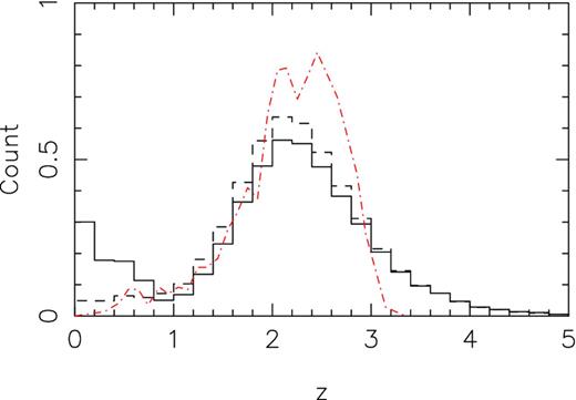
The estimated redshift distributions found by using our method and applying the cuts used by Amblard et al. (2010): S350 > 35 mJy, S250 and S500 > 3σ. The solid black line shows our predicted redshift distribution if we use the redshifts of the reliable optical counterparts in preference to those estimated from the Herschel fluxes. The black dashed line shows the results of using only the redshifts estimated from the Herschel fluxes. In the first case, we find a mean redshift of z = 2.0. The red dot–dashed line shows the redshift distribution obtained by Amblard et al. (2010).
We also include in Fig. 11 our distribution of predicted redshifts if we now ignore the redshifts of any optical counterparts. In this case, we see no low-redshift peak and a mean z = 2.3 in good agreement with what Amblard et al. (2010) found. One possible explanation of the disappearance of the low-redshift peak are that these sources are mostly lensed high-redshift Herschel sources.
Lapi et al. (2011) used an S250 μm > 35 mJy, S350 μm > 3σ selection on SDP sources without an optical counterpart, again biasing against low-z sources. Three reference SEDs from galaxies at z = 0.018, 2.3 and 4.2 were used to estimate redshifts from these fluxes and all produced similar distributions with a broad peak at 1.5 ≲ z ≲ 2.5 and a tail up to z ≈ 3.5. Using our template and these same cuts, we find a mean of z = 1.8 (see Fig. 12). Our and Lapi's estimates for the ztemp distribution are very similar. This also confirms that the methods of both Lapi et al. (2011) and González-Nuevo et al. (2012) are reliable for estimating the redshifts of high-z sources. Lapi et al. (2011) present a model for the formation of early-type galaxies that gives much better agreement with the estimated redshift distribution of H-ATLAS galaxies at z > 1.
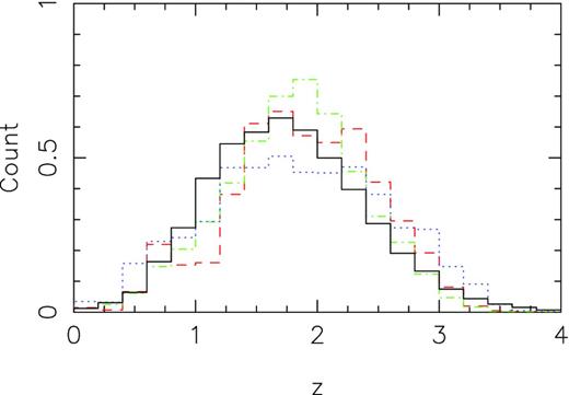
The estimated redshift distributions found by using our template and applying the cuts used by Lapi et al. (2011): S250 > 35 mJy, S350 > 3σ, no optical counterpart; solid black. The other lines shows the redshift distributions found by Lapi et al. (2011) for the H-ATLAS SDP field, the red dashed line with SMM J2135−0102 as the template, the green dot–dashed line with G15.141 as the template and the blue dotted line with Arp 220 as the template.
5 CONCLUSIONS
We generated a template for estimating the redshift of H-ATLAS galaxies using a sample of H-ATLAS galaxies with measured redshifts. Our best-fitting template consists of two dust components with Th = 46.9 K, Tc = 23.9 K, β = 2 and the ratio of cold dust mass to warm dust mass of 30.1. To estimate the uncertainty in the template, we used a jackknife technique and found a mean Δz/(1 + z) = 0.03 with an rms of 0.26. If there is some a priori knowledge that the source is at z > 1, we estimate a mean Δz/(1 + z) = 0.013 with an rms or 0.12.
This template was then used to estimate the redshifts of the entire H-ATLAS Phase 1 sources, though optical redshifts were used where available. Our redshift distributions show two peaks, suggesting there are two populations of sources experiencing different cosmological evolution. The mean redshifts for sources detected at >5σ at three wavelengths are 1.2, 1.9 and 2.6 for 250, 350 and 500 μm selected sources, respectively.
The Herschel-ATLAS is a project with Herschel, which is an ESA space observatory with science instruments provided by European-led Principal Investigator consortia and with important participation from NASA. The H-ATLAS website is http://www.h-atlas.org/. GAMA is a joint European-Australasian project based around a spectroscopic campaign using the Anglo-Australian Telescope. The GAMA input catalogue is based on data taken from the SDSS and the UKIRT Infrared Deep Sky Survey. Complementary imaging of the GAMA regions is being obtained by a number of independent survey programmes including GALEX MIS, VST KIDS, VISTA VIKING, WISE, Herschel-ATLAS, GMRT and ASKAP providing UV to radio coverage. GAMA is funded by the STFC (UK), the ARC (Australia), the AAO and the participating institutions. The GAMA website is http://www.gama-survey.org/. SPIRE has been developed by a consortium of institutes led by Cardiff University (UK) and including Univ. Lethbridge (Canada); NAOC (China); CEA, LAM (France); IFSI, Univ. Padua (Italy); IAC (Spain); Stockholm Observatory (Sweden); Imperial College London, RAL, UCL-MSSL, UKATC, Univ. Sussex (UK); and Caltech, JPL, NHSC, Univ. Colorado (USA). This development has been supported by national funding agencies: CSA (Canada); NAOC (China); CEA, CNES, CNRS (France); ASI (Italy); MCINN (Spain); SNSB (Sweden); STFC (UK) and NASA (USA). KSS is supported by the National Radio Astronomy Observatory, which is a facility of the National Science Foundation operated under cooperative agreement by Associated Universities, Inc. JGN acknowledges financial support from Spanish CSIC for a JAE-DOC fellowship and partial financial support from the Spanish Ministerio de Ciencia e Innovacion project AYA2010-21766-C03-01.
Herschel is an ESA space observatory with science instruments provided by European-led Principal Investigator consortia and with important participation from NASA.
www.h-atlas.org
