


Abstract
We discuss the detection of large-scale H i intensity fluctuations using a single dish approach with the ultimate objective of measuring the baryonic acoustic oscillations (BAO) and constraining the properties of dark energy. To characterize the signal we present 3D power spectra, 2D angular power spectra for individual redshift slices and also individual line-of-sight spectra computed using the S3 simulated H i catalogue which is based on the Millennium Simulation. We consider optimal instrument design and survey strategies for a single dish observation at low and high redshift for a fixed sensitivity. For a survey corresponding to an instrument with Tsys = 50 K, 50 feedhorns and 1 year of observations, we find that at low redshift (z ≈ 0.3), a resolution of ∼40 arcmin and a survey of ∼5000 deg2 is close to optimal, whereas at higher redshift (z ≈ 0.9) a resolution of ∼10 arcmin and ∼500 deg2 would be necessary – something which would be difficult to achieve cheaply using a single dish. Continuum foreground emission from the Galaxy and extragalactic radio sources are potentially a problem. In particular, we suggest that it could be that the dominant extragalactic foreground comes from the clustering of very weak sources. We assess its amplitude and discuss ways by which it might be mitigated. We then introduce our concept for a dedicated single dish telescope designed to detect BAO at low redshifts. It involves an underillumintated static ∼40 m dish and a ∼60 element receiver array held ∼90 m above the underilluminated dish. Correlation receivers will be used with each main science beam referenced against an antenna pointing at one of the celestial poles for stability and control of systematics. We make sensitivity estimates for our proposed system and projections for the uncertainties on the power spectrum after 1 year of observations. We find that it is possible to measure the acoustic scale at z ≈ 0.3 with an accuracy ∼2.4 per cent and that w can be measured to an accuracy of 16 per cent.
INTRODUCTION
Precision cosmology is now a reality. Measurements of the cosmic microwave background (CMB), large-scale structure (LSS) and Type Ia supernovae have led the way in defining the standard cosmological model, one based on a flat Friedmann–Robertson–Walker Universe containing cold dark matter (CDM) and a cosmological constant, Λ, with densities relative to the present-day critical density Ωm ≈ 0.27 and ΩΛ ≈ 0.73 (Riess et al. 1998; Perlmutter et al. 1999; Eisenstein et al. 2001; Percival et al. 2002; Komatsu et al. 2011). The standard model has just six parameters, but these can been expanded to constrain, rule out or detect more exotic possibilities. One particular case is an expanded dark energy sector, often parametrized by the equation-of-state parameter w = P/ρ for the dark energy (Copeland, Sami & Tsujikawa 2006), or even the possibility of modifications to gravity (Clifton et al. 2011). Observations which can constrain the dark sector are usually geometrical (standard rulers or candles) or based on constraining the evolution of structure (Weinberg et al. 2012).
The use of baryonic acoustic oscillations (BAOs) to constrain w is now an established technique (Eisenstein, Hu & Tegmark 1998; Eisenstein 2003). Originally applied to the Third Data Release (DR3) of the Sloan Digital Sky Survey (SDSS) luminous red galaxy survey (Eisenstein et al. 2005), subsequent detections have been reported by a number of groups analysing data from Two degree Field (2dF; Percival et al. 2001; Cole et al. 2005), SDSS DR7 (Percival et al. 2010), WiggleZ (Blake et al. 2011), Six degree Field (6dF; Beutler et al. 2011) and Baryon Oscillation Spectroscopic Survey (BOSS; Anderson et al. 2012). All these have used redshift surveys performed in the optical waveband to select galaxies. The power spectrum of their 3D distribution is computed and, assuming that the power spectrum of the selected galaxies is only biased relative to the underlying dark matter distribution by some overall scale-independent constant, the acoustic scale can then be extracted. Present sample sizes used for the detection of BAOs are typically ∼105 galaxies, but there are a number of projects planned to increase this to ∼107–108 using optical and near-infrared (NIR) observations which would lead to increased levels of statistical precision (Abbott et al. 2005; Hawken et al. 2011; Laureijs et al. 2011; Schlegel et al. 2011).
It is possible to perform redshift surveys in the radio waveband, using 21 cm radiation from neutral hydrogen (H i) to select galaxies which could provide improved confidence in the results from the optical/NIR. At present the largest surveys have only detected ∼104 galaxies (Meyer et al. 2004), limited by the low luminosity of the 21 cm line emission (Furlanetto, Oh & Briggs 2006; Morales & Wyithe 2009), but there are a number of proposed instruments with large collecting area capable of increasing this substantially in the next decade (Abdalla & Rawlings 2005; Duffy et al. 2008; Abdalla, Blake & Rawlings 2010). By the time the Square Kilometre Array (SKA)1 is online the redshift surveys of galaxies selected in the radio should have comparable statistical strength to those made in the optical/NIR. The advantage of doing both radio and optical surveys is that they will be subject to completely different systematics.
An intriguing possibility is the idea of using what has become known as 21 cm intensity mapping. The fact that the 21 cm line is so weak means that it requires ∼1 km2 of collecting area to detect L⋆ galaxies at z ∼ 1 in an acceptable period of time – this was the original rationale for the SKA (Wilkinson 1991). However, instruments with apertures of ∼100 m size have sufficient surface brightness sensitivity to detect H i at higher redshift, but they will preferentially detect objects of angular size comparable to their resolution as pointed out in Battye, Davies & Weller (2004). These objects will be clusters with masses 1014–1015 M⊙ and other LSS. Peterson, Bandura & Pen (2006) and Loeb & Wyithe (2008) suggested that the full intensity field T(θ, ϕ, f) could be used to measure the power spectrum as a function of redshift directly (as is done for the CMB intensity fluctuations) if the smooth continuum emission, e.g. that from the Galaxy, can be accurately subtracted and any systematic instrumental artefacts, arising from the observational strategy, can be calibrated to sufficient accuracy. If these obvious difficulties can be mitigated, then this technique can be enormously powerful: the standard approach of detecting galaxies and then averaging them to probe LSS is inefficient in the sense that to detect the galaxies, at say 5σ, one throws away all but a fraction of the detected 21 cm emission. Although this is not a problem in the optical, in the radio where the signal is much weaker one cannot afford to take this hit. In order to measure the power spectrum one is not trying to detect the actual galaxies, although this can lead to a plethora of other legacy science, and all the detected emission is related to the LSS structure. Chang et al. (2008) have shown that dark energy can be strongly constrained with a radio telescope significantly smaller, and cheaper, than the SKA.
Interferometric techniques naturally deal with some of the issues related to foregrounds and instrumental systematics. In particular, they can filter out more efficiently the relatively smooth and bright contaminating signals from the Galaxy and local signals such as the Sun, Moon and ground. However, interferometers can be extremely expensive since they require electronics to perform the large number of correlations. In this paper, we will present our ideas on the design of a single dish telescope and an analysis of its performance (BAO from Integrated Neutral Gas Observations, BINGO). A single dish instrument would provide the simplest and cheapest way of achieving a particular surface brightness sensitivity. Attempts have already been made to detect the signal using presently operational, single-dish radio telescopes (Chang et el. 2010; Switzer et al. 2013) and recent surveys of the local Universe (Pen et al. 2009). It has been possible to make detections using cross-correlation with already available optical redshift surveys, but not the detection of the crucial autocorrelation signal needed to probe cosmology using radio observations alone. The reasons for this are unclear, but they are likely to be due to a combination of the observations not been taken with this specific purpose in mind and the fact that the telescope and detector system are not sufficiently stable. Our philosophy in this paper will be to quantify the expected H i signal, quantify the contaminating foreground signals and then present our design for a system which will be sufficiently sensitive and stable for the BAO signal to be extracted.
CHARACTERIzATION OF THE SIGNAL
In this section, we will present some basic material on the 21 cm line emission in order to characterize various aspects of the signal expected in a H i intensity mapping experiment.
Mean temperature
Throughout we will assume that |$\Omega _{\rm H\,{\small {I}}}h=2.45\times 10^{-4}$| independent of redshift which is the value calculated from the local H i mass function measured by HI Parkes All Sky Survey (HIPASS; Zwaan et al. 2005). Both observational (Prochaska & Wolfe 2009) and theoretical arguments (Duffy et al. 2012) appear to suggest that there is no more than a factor of 2 change in density of neutral hydrogen over the range of redshifts relevant to intensity mapping. In the rest of the paper, we will drop the “obs’ subscript and use T to denote the observed brightness temperature.
3D power spectrum
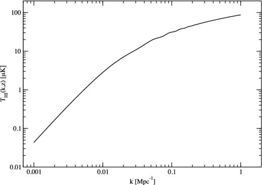
The 3D H i power spectrum at z = 0.28. BAOs are just about visible in the range 0.01 < k/Mpc−1 < 0.2, but they are less than 10 per cent of the total signal. For k < 0.01 Mpc−1 the temperature spectrum is ∝k2 corresponding to P(k) ∝ k, that is, scale invariant.
2D angular power spectrum
In Fig. 2, we plot the H i angular power spectra for the same central frequency 950 MHz (corresponding to a central redshift zc ≈ 0.5) but for two different bin widths Δf = 300 and 50 MHz. We see that as a result of decreasing the bin size, the signal amplitude increases and the BAO wiggles become more prominent. It is clear that there exists an optimum frequency bin size for which a detection will be possible: the signal-to-noise ratio level would increase |$\propto \sqrt{\Delta f}$| if the signal level was independent of frequency, but the level of fluctuations in the H i is reduced as the box enclosed by the angular beam-size and frequency range are increased. In Fig. 3, we plot the ratio Cℓ/Cℓ, smooth, where Cℓ, smooth is the no-wiggles angular power spectrum (Eisenstein & Hu 1998) for the same central frequency 950 MHz but for the two frequency ranges used in Fig. 2. In addition we have plotted the ratio P(k)/Psmooth(k), where P(k) = Pcdm(k). Note that the ratio Cℓ/Cℓ, smooth cannot be bigger than P(k)/Psmooth(k). However, the two are in close agreement for the Δf = 50 MHz bin which indicates that this is the optimal frequency bin size for tracing the BAOs.
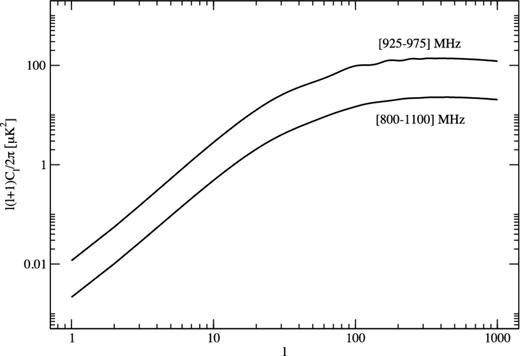
The H i angular power spectrum for the same central frequency, 950 MHz, but for two different ranges 925–975 MHz and 800–1100 MHz. The signal amplitude increases with decreasing the frequency range and the BAOs become more prominent. As the frequency range increases the size of the region probed becomes larger implying that the fluctuations will decrease.
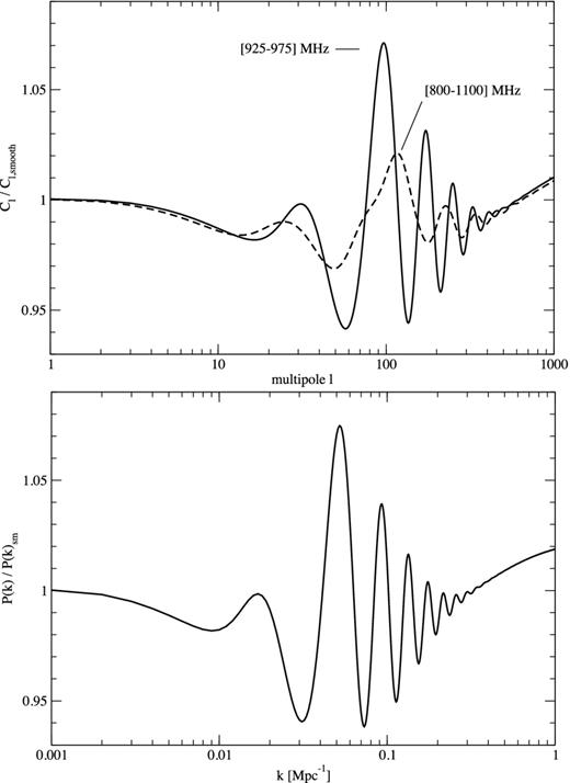
In the top plot, we present the ratio Cℓ/Cℓ, smooth for the same central frequency (950 MHz) but for different frequency ranges. In the bottom plot, we present the ratio P(k)/P(k)smooth. The 925–975 MHz curve in the upper plot is very similar to that in the lower one implying that a frequency range of 50 MHz will be optimal to detect the BAO signal at this redshift.
Estimated signal from S3 simulations
Obreschkow et al. (2009a,b) present semi-analytic simulations of H i emission based on catalogues of galaxies whose properties are evolved from the Millennium or Milli-Millennium dark matter simulations (Springel et al. 2005) and we will use these to compute simulated spectra as would be observed by a single dish. We adopt the smaller of the two resultant mock sky fields (corresponding to the Milli-Millennium simulation, comoving diameter sbox = 62.5 h−1 Mpc) for the characterization of the expected H i signal which, as we will discuss later, restricts the highest redshift to which the spectrum will be complete. We extract galaxy properties from the simulated catalogue – position coordinates, redshift, H i mass, integrated H i flux and H i-line width – from which we calculate the H i brightness temperature contributed by galaxies in the frequency range Δf, as it would be observed by a telescope beam which is a top hat of diameter θFWHM independent of frequency. Using a diffraction limited beam for which θFWHM ∝ 1 + z would result in a higher signal at lower frequencies.
In Fig. 4, we present the expected H i temperature fluctuations between frequencies of 800 and 1200 MHz, which is part of the frequency range we will be interested in, for a range of beam sizes, θFWHM and frequency bandwidths, Δf. These plots provide considerable insight into the nature of the signal that we will be trying to detect. It appears that the average signal from equation (9), represented by the dashed line, is compatible with the spectra from the Millennium Simulation. Larger values of θFWHM and Δf mean that the volume of the universe enclosed within a single cell is larger and hence the spectra have only very small deviations from the average, whereas for smaller values there are significant deviations as large as 400 μK illustrating that the signal on these scales can be much higher than the average.
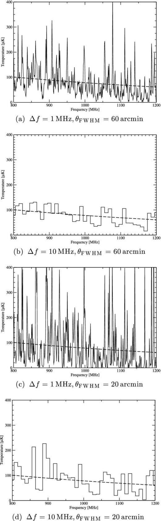
The simulated H i signal for different telescope beam resolution and frequency bin size combinations, θFWHM and Δf, respectively. A smaller frequency bin or telescope beam size results in larger fluctuations, as expected, since going to smaller values of θFWHM and Δf means that one is probing a smaller volume of the Universe and fluctuations in the H i density are expected to be larger on smaller scales, as they are in the CDM. In each case, the dashed line is the average temperature computed using (9). The objective of 21 cm intensity mapping experiments is to measure the difference between the signal and this average. (a) Δf = 1 MHz, θFWHM = 60 arcmin. (b) Δf = 10 MHz, θFWHM = 60 arcmin. (c) Δf = 1 MHz, θFWHM = 20 arcmin. (d) Δf = 10 MHz, θFWHM = 20 arcmin.
There are limitations to this approach: our spectra are not accurate out to arbitrarily high redshift where the cone diameter exceeds sbox and hence simulated catalogue is missing galaxies, that is, it is not complete. The maximum redshift for which the simulated catalogue is complete is determined by the beam size, with smaller beam sizes being accurate to higher redshifts. For a beam size of 1°, the spectrum will be accurate up to around 600 MHz.
At the other end of the frequency range, which is not shown in Fig. 4, there are large fluctuations around the mean that can be attributed to the effects of shot noise. In Fig. 5, we plot the number of galaxies contributing to each bin of the spectrum defined by θFWHM = 20 arcmin and Δf = 1 MHz, that is, Fig. 4(c), as a function of redshift. At low redshifts (high frequencies) the number of galaxies contributing to each bin is small, and the signal cannot be thought of as an unresolved background. If N is the number of contributing galaxies, the deviation due to shot noise is σ2 ∝ 1/N and consequently, we see larger fluctuations. This is exactly the regime probed by surveys such as HIPASS and Arecibo Legacy Fast ALFA (ALFALFA), which detect individual galaxies for z < 0.05 with slightly better – but not substantially better – resolution than used in this plot. As one moves to higher redshifts a low-resolution telescope will preferentially detect objects which have an angular size which is similar to that of the beam. At intermediate redshifts these will be the clusters discussed in Battye et al. (2004) and these can be clearly seen as the well-defined spikes in the spectrum around z = 0.3-0.4. At higher redshifts even clusters are beam diluted; beyond z = 0.5 there are always a few galaxies contributing to each bin – essentially there is an unresolved background.
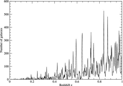
The number of galaxies contributing to the H i signal in each bin as a function of redshift. We have used θFWHM = 20 arcmin and Δf = 1 MHz for this particular example. Note that the signal presented in Fig. 4 varies only very weakly with redshift yet the number of galaxies contributing to each bin increases dramatically. At low redshifts, we see that the signal is dominated by individual galaxies, at intermediate redshifts it is dominated by galaxy clusters and groups as suggested in Battye et al. (2004) and at high redshifts the signal comprises an unresolved background signal, that is, there are a very large number of galaxies contributing to each bin in redshift.
We can quantify the H i temperature fluctuations as a function of θFWHM and Δf by calculating their root mean squared (rms) deviation about the mean over the frequency range. As shown in Fig. 6, the rms decreases with increasing θFWHM and Δf. This is exactly what is expected since as θFWHM and Δf increase, the region of the Universe enclosed is larger and the observed temperature will become closer to the average. We note that typically the fluctuations are significantly bigger than one for a substantial part of the parameter space.
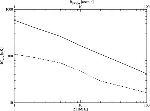
The rms temperature fluctuations in the H i signal as a function of θFWHM (solid line) and Δf (dashed line). When we vary θFWHM, we fix Δf = 1 MHz and in the case where Δf is varied we fix θFWHM = 20 arcmin.
OPTIMIZING THE PERFORMANCE AND SCIENCE POTENTIAL OF A SINGLE DISH EXPERIMENT
In this section, we analyse the expected performance of a single dish telescope in two frequency ranges either side of the mobile phone band around 900-960 MHz: (A) f = 960-1260 MHz (0.13 < z < 0.48) and (B) f = 600-900 MHz (0.58 < z < 1.37). We will compute projected error bars on the resulting power spectra based on the methods presented in Seo et al. (2010) using the 3D power spectrum (1). In each case, (A) and (B), we will optimize the area covered, Ωsur, and the resolution of the telescope, θFWHM ∝ 1/D, where D is the illuminated area of the dish, in order to give the best possible measurement of the acoustic scale.
In Figs 7 and 8 we present projected percentage errors on the acoustic scale, 100δkA/kA as a function of the survey area, Ωsur, and the beam size, θFWHM for the redshift ranges given by cases A and B. First it is clear that in each case there are a wide range of survey parameters for which accurate measurements of kA can be made. It will always be the case that reducing θFWHM will lead to a better measurement of kA. However, beyond some point one gets into a situation where there is a very significant extra cost for very little extra return.
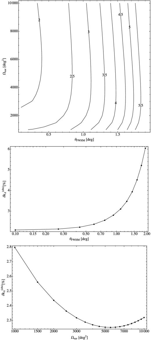
Optimization of the measurement of kA for case (A) – observations over the frequency range 960-1260 MHz. We have computed the projected uncertainty on the measurement of kA as a function of ΔΩsur and the beam size θFWHM. In the top panel, the contours are lines of constant δkA with the numbers on the contours signifying the percentage fractional error: 100δA/kA. In the middle panel, we present a 1D slice as a function of θFWHM with ΔΩsur = 2000 deg2 and in the bottom panel a 1D slice as a function of Ωsur with θFWHM = 40 arcmin.
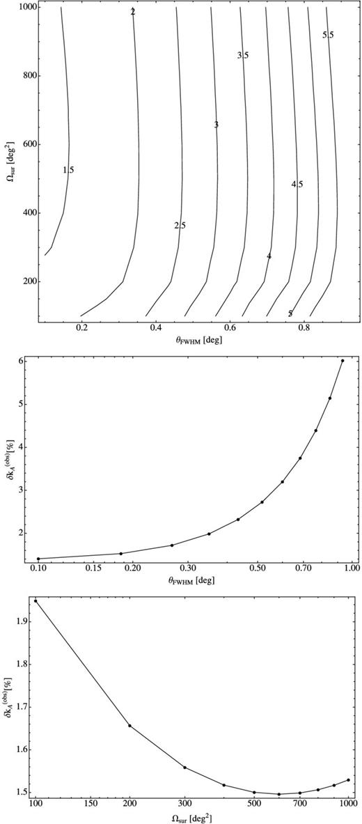
Optimization of the measurement of kA for case (B) – observations over the frequency range 600-900 MHz. We have computed the projected error on the measurement of kA as a function of ΔΩsur and the beam size θFWHM. In the top panel, the contours are lines of constant δkA. The numbers on the contours are defined in the same way as in Fig. 7. In the middle panel, we present a 1D slice as a function of θFWHM with ΔΩsur = 500 deg2 and in the bottom panel a 1D slice as a function of Ωsur with θFWHM = 10 arcmin.
In case A, for Ωsur > 2000 deg2 the contours of constant δkA/kA are almost vertical. This implies that for a fixed value of θFWHM, as long as one can achieve Ωsur > 2000 deg2, optimization of the survey area can only yield minor improvements. This is illustrated in the bottom panel of Fig. 7, where we fixed θFWHM. The optimum Ωsur is between 5000 and 6000 deg2 where δkA/kA ≈ 0.0225, but for example if Ωsur = 2000 deg2, as we will suggest for the BINGO instrument discussed in Section 5, δkA/kA ≈ 0.024, a difference which is within the uncertainties of the present calculations. The exact position of the optimum is governed by a balance between cosmic variance and thermal noise terms in equation (22); typically, it is where the two are approximately equal. In the middle panel of Fig. 7, we fix Ωsur = 2000 deg2 and vary only θFWHM. There is a significant improvement in δkA/kA as one goes from θFWHM = 2° to around 40 arcmin but beyond that point there is little improvement. The reason for this is made apparent in Fig. 9 where we present the projected errors on P(k)/Psmooth(k), where Psmooth(k) is a smooth power spectrum chosen to highlight the BAOs. We see that as one goes to higher values of k, corresponding to higher angular resolution and lower values of θFWHM, the overall amplitude of the BAO signal decreases and therefore it is clear that the discriminatory power, in terms of measuring BAOs2 comes from the first three oscillations in the power spectrum. Although measuring beyond this point will improve the constraint, the improvement does not justify the substantial extra cost involved; going from θFWHM = 40 to 20 arcmin would require the telescope diameter to increase by a factor of 2 and the cost by a factor of somewhere between 5 and 10. For the subsequent discussion of case A, we will concentrate on θFWHM = 40 arcmin and Ωsur = 2000 deg2 and the relevant survey parameters are presented in Table 1. This is not exactly the optimum point in the θFWHM-Ωsur plane, but it is sufficiently close to the optimum. θFWHM = 40 arcmin can be achieved with an illuminated diameter of around 25 m at the relevant frequencies and Ωsur = 2000 deg2 can be achieved with a drift scan strip of around 10° at moderate latitudes which is compatible with our choice of Δk. We note that the precise values of the optimum depend on the overall survey speed which is governed by |$t_{\rm obs}n_{\rm F}/T_{\rm sys}^2$|. Typically, an increase in the overall survey speed will move the optimum survey area to a larger value.
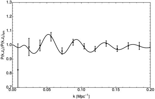
Projected errors on the power spectrum (divided by a smooth power spectrum) expected for the survey described by the parameters used in the text and Table 1 which is close to the optimal value for Fig. 7, that is, case (A) from Table 1. We have used Δk = 0.016 Mpc−1. The projected errors would lead to a measurement of the acoustic scale with a percentage fractional error of 2.4 per cent. Note that the points do not lie on the line since they are band powers and hence are integrals over neighbouring values of k.
Shows survey parameters used in Figs 9 and 10. In both cases, we have chosen the values of θFWHM and Ωsur so as to be close the optimal values as described in the text. Included also are the projected measurements of the acoustic scale and estimates of the error w (assumed constant) when all other cosmological parameters are known.
| Property | Low redshift (A) | High redshift (B) |
|---|---|---|
| zcentre | 0.28 | 0.9 |
| r(zcentre) | 1100 Mpc | 3000 Mpc |
| Ωsur | 2000 deg2 | 500 deg2 |
| Vsur | 1.2 Gpc3 | 3.1 Gpc3 |
| θFWHM | 40 arcmin | 10 arcmin |
| Vpix | 810 Mpc3 | 590 Mpc3 |
| rms noise level (Δf = 1 MHz) | 85 μK | 170 μK |
| δkA/kA | 0.024 | 0.015 |
| δw/w | 0.16 | 0.07 |
The situation for case (B) is qualitatively similar, but the exact values are somewhat different. Being centred at a much higher redshift, z ≈ 0.9, means that the angular size of the BAO scale is much smaller and hence higher resolution is necessary to resolve the BAO scale and a smaller area needs to be covered to achieve the same balance between thermal noise and cosmic variance. We find that something close to optimal can be achieved for θFWHM = 10 arcmin and Ωsur = 500 deg2, which is compatible with the analysis of Masui et al. (2010). The projected errors for such a configuration are displayed in Fig. 10 which would lead to δkA/kA ≈ 0.015. In order to achieve this, one would need a single dish telescope with an illuminated diameter of ∼100 m which would have to be steerable, at least in some way. It would be relatively expensive to build a dedicated facility to perform such a survey, although, of course, such facilities do already exist, albeit with very significant claims on their time from other science programmes. Perhaps an interferometric solution could be used to achieve this optimum: we find that an array of ∼250 antennas with a diameter of 4 m spread over a region of diameter ∼100 m, having the same value Tsys, could achieve the same level of sensitivity. More generally an interferometer comprising nd antennas of diameter D spread over a region of diameter d would be equivalent to a single dish of diameter d with a focal plane array with nF feedhorns, if |$n_{\rm d}=d\sqrt{n_{\rm F}}/D$| so long as nF < nd, that is the filling factor of the interferometer is <1.
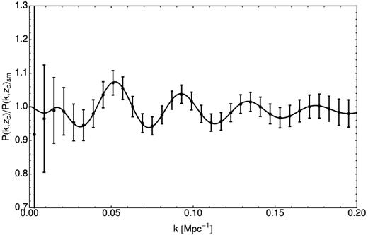
Projected errors on the power spectrum (divided by a smooth power spectrum) expected for the survey described by the parameters used in the text and Table 1 which is close to the optimal value for Fig. 8, that is case (B) from Table 1. We have used Δk = 0.006 Mpc−1. The projected errors would lead to a measurement of the acoustic scale with a percentage fractional error of 1.5 per cent.
In order to get an impression of the science reach of the proposed observations we have done two things. First, in Fig. 11 we have plotted our projected constraints on the angle-averaged distance on the BAO Hubble diagram – both absolute and residuals – along with the state-of-the-art measurements from 6dF, SDSS-II, BOSS and WiggleZ. It is clear that the measurements that would be possible from instruments capable of achieving the design parameters of cases A and B would be competitive with the present crop of observations and those likely to be done in the next few years. They would also be complementary in terms of redshift range and add to the possibility of measuring the cosmic distance scale solely from BAOs. We note that it should be possible, in fact, to make measurements of the acoustic scale over the full range of redshifts probed by the intensity mapping surveys and it would be possible to place a number of data points on the Hubble diagram, albeit with larger error bars. In order to compare with the present surveys we decided to present a single data point.
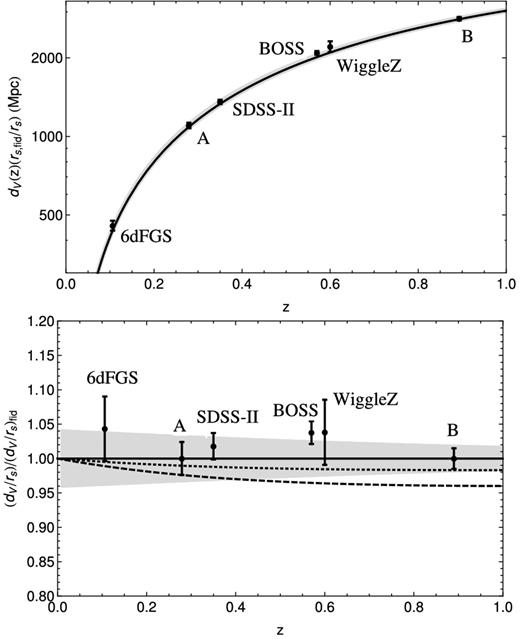
Projected constraints on the Hubble diagram for the volume averaged distance, dV(z), for cases A and B described by the parameters in Table 1. Included also are the actual measurements made by 6dF, SDSS-II, BOSS and WiggleZ. The top panel is the absolute value and the bottom panel are the residuals from the fiducial model. In the bottom panel, the shaded region indicates the range of dV allowed by the 1σ constraint Ωmh2 from WMAP7 (Komatsu et al. 2011). The dotted line is the prediction for w0 = −0.84 (which could in principle be ruled out by case A) and the dashed line is w0 = −0.93 (by case B).
In addition, we have made simple estimates of the projected errors of the dark energy parameters assuming that all the other cosmological parameters, including Ωm are fixed. This will be a good approximation in the era of high precision CMB measurements made by, for example, the Planck satellite.3 For constant w, the measurement of δkA/kA = 0.024 possible in case A would lead to δw/w = 0.16, whereas for case B, where δkA/kA = 0.015 would lead to δw/w = 0.07. For models with non-constant w, we have performed a simple likelihood analysis for the 2D parameter space w0-w1 and the results are presented in Fig. 12 for cases A and B and a combination of the two. We see that since we have assumed a single redshift measurement of the acoustic scale, there is an exact degeneracy between the two parameters, but the direction of the degeneracy is very different at the two different redshifts. When they are combined the degeneracy is broken and it is possible to estimate the two parameters separately.
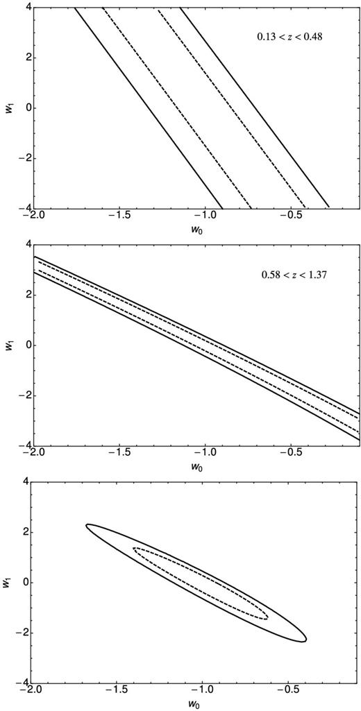
Projected uncertainties on the dark energy parameters w0 and w1 for case A with θFWHM = 2/3 deg and Ωsur = 2000 deg2 (top), case B with θFWHM = 10 arcmin and Ωsur = 500 deg2 (middle) and a combination of the two (bottom) for the case where all other cosmological parameters are known. We have assumed that cases A and B lead to a measurement of the acoustic scale at the central redshift of the survey which means that there is an absolute parameter degeneracy between the two parameters, but the degenerate line is different at the two redshifts. Combination of the two removes the degeneracy.
FOREGROUND CONTAMINATION
Overview
The foregrounds will be much brighter than the H i signal, by several orders of magnitude. At f = 1 GHz, |$\bar{T}_{\rm sky} \sim 5$| K, while the H i brightness temperature is ∼0.1 mK. However, our objective is to measure fluctuations of the sky brightness temperature as a function of both angular scale and redshift. Fluctuations of the H i signal are expected to be at the same level as the smooth component (|$\delta T_{\rm H\,{\small {I}}} \sim \bar{T}_{\rm H\,{\small {I}}} \sim 0.1$| mK), while the fluctuations of the foregrounds will typically be much less (|$\delta T \ll \bar{T}$|). Furthermore, we can choose the coldest regions of sky to minimize the foreground signal. We will show that regions exist where the fluctuations in the foregrounds are in fact a little less than two orders of magnitude brighter than the H i signal. Given that the foregrounds will be smooth in frequency, this gives us confidence that foreground separation algorithms (e.g. Liu & Tegmark 2011) can be employed that will allow a detection of BAO.
Estimates of the foreground brightness temperature fluctuations are presented in the next sections for each component and are summarized in Table 2.
Summary of foregrounds for H i intensity mapping at 1 GHz for an angular scale of ∼1° (ℓ ∼ 200). The estimates are for a 10° wide strip at declination δ = +45° and for Galactic latitudes |b| > 30°.
| Foreground | |$\bar{T}$| | δT | Notes |
|---|---|---|---|
| (mK) | (mK) | ||
| Synchrotron | 1700 | 67 | Power-law spectrum with β ≈ −2.7. |
| Free–free | 5.0 | 0.25 | Power-law spectrum with β ≈ −2.1. |
| Radio sources (Poisson) | – | 5.5 | Assuming removal of sources at S > 10 mJy. |
| Radio sources (clustered) | – | 9.1 | Assuming removal of sources at S > 10 mJy. |
| Extragalactic sources (total) | 205 | 10.6 | Combination of Poisson and clustered radio sources. |
| CMB | 2726 | 0.07 | Blackbody spectrum, (β = 0). |
| Thermal dust | – | ∼2 × 10⁻⁶ | Model of Finkbeiner, Davis & Schlegel (1999). |
| Spinning dust | – | ∼2 × 10⁻³ | Davies et al. (2006) and CNM model of Draine & Lazarian (1998). |
| RRL | 0.05 | 3 × 10⁻³ | Hydrogen RRLs with Δn = 1. |
| Total foregrounds | ∼4600 | ∼67 | Total contribution assuming that the components are uncorrelated. |
| H i | ∼0.1 | ∼0.1 | Cosmological H i signal we are intending to detect. |
Galactic synchrotron radiation
At frequencies ∼1 GHz observations indicate that synchrotron emission is well approximated by a power law with spectral indices in the range −2.3 to −3.0 (Reich & Reich 1988). The mean value |$\bar{\beta } \approx -2.7$| and mean dispersion σβ = 0.12 are measured by Platania et al. (2003) in the range 0.4–2.3 GHz.
A number of large-area surveys are available at frequencies of ∼1 GHz, most notably the all-sky 408 MHz map of Haslam et al. (1982). We use the NCSA destriped and source-removed version of this map4 to estimate the contribution of synchrotron emission at 1 GHz. The 408 MHz map is extrapolated to 1 GHz using a spectral index of β = −2.7. The map is shown in right ascension–declination coordinates in Fig. 13. The Galactic plane is evident as well as large-scale features that emit over large areas of the high latitude sky. The most prominent feature is the North Polar Spur which stretches over ∼100° of the northern sky. The mean temperature at high Galactic latitudes (|b| > 30°) is Tsky ≈ 2 K with rms fluctuations in maps of 1° resolution of δTGal ≈ 530 mK. The rms fluctuations are dominated by contributions from the large-scale features.
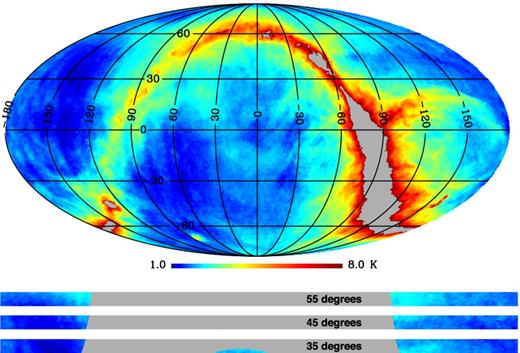
In the top plot, we present the entire synchrotron sky in celestial (RA/Dec.) coordinates, with RA = 0° at the centre and increasing to the left. The map has been extrapolated from the all-sky 408 MHz map (Haslam et al. 1982) to 1 GHz using a spectral index β = −2.7 (Platania et al. 2003). The colour scale is a sin h from 1 to 8 K. The saturated pixels (T > 8 K) are shown as grey. In the bottom plot, we present three drift scan strips, each 10° wide, located at declinations of 35° (bottom), 45° (middle) and 55° (top).
Fortunately, there exist large areas of low synchrotron temperature in the north. The declination strip at δ ∼ +40° is well known to be low in foregrounds (Davies, Watson & Gutierrez 1996) and is accessible by observing sites in the north. Furthermore, we are interested in the fluctuations at a given angular scale, or multipole value ℓ, rather than the rms value in the map at a given resolution. The rms estimate from the map will be considerably larger due to fluctuations on larger angular scales than the beam.
To estimate the foreground signal at a given ℓ value we calculated the power spectrum of the δ = +45° strip after masking out the Galactic plane (|b| > 30°). This was achieved by using the polspice5 software, which calculates the power spectrum from the two-point pixel correlation function (Szapudi, Prunet & Colombi 2001; Chon et al. 2004). We apodized the correlation function with a Gaussian of width σ = 10° to reduce ringing in the spectrum at the expense of smoothing the spectrum. A power-law fit was then made to estimate the foreground signal at ℓ = 200 (∼1°). The result is given in Table 2.
For a 10° wide strip centred at δ = 45° we find that the |$\bar{T}_{\rm Gal}=1.7$| K with fluctuations of δTGal = 67 mK. Utilizing these cool regions will be important for detecting the faint H i signal. The exact choice of strip will be a critical factor to be decided before construction of a fixed elevation telescope while the Galactic mask to be applied can be chosen during the data analysis step.
Free–free radiation
The EM can be estimated using Hα measurements, which can then be converted to radio brightness temperature assuming that Te is known and the dust absorption is small (Dickinson, Davies & Davis 2003). For |b| > 30°, where Te ≈ 8000 K, EM ∼ 1.3 cm−6 pc at 1 GHz, this corresponds to |$\bar{T}_{\rm ff} \sim 5$| mK. For the 10° wide strip at δ = +45° the free–free brightness temperature fluctuations are δTff = 0.25 mK at ℓ = 200. The free–free component is therefore considerably weaker than the synchrotron component across most of the sky, but will act to (slightly) flatten the spectrum at higher frequencies.
Extragalactic foregrounds
Extragalactic radio sources are an inhomogeneous mix of radio galaxies, quasars and other objects. These contribute an unresolved foreground.6 The sources are often split into two populations based on their flux density spectral index, α (S ∝ να): steep spectrum sources with α < −0.5 and flat spectrum sources with α > −0.5. At low frequencies (≲1 GHz), steep spectrum sources with α ≈ −0.75 will dominate (Kellermann, Paulint-Toth & Davis 1968).
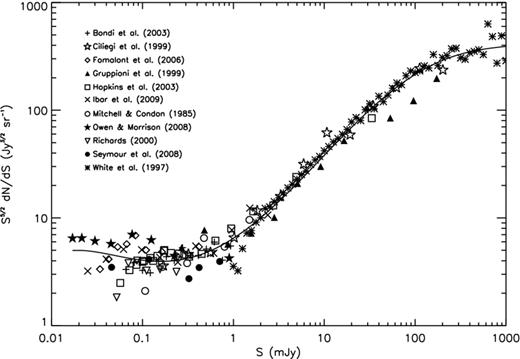
The compilation of differential radio sources counts at 1.4 GHz which we have used. The solid line is the best-fitting fifth-order polynomial.
References used for source surveys at ∼1.4 GHz used for compilation of source counts.
| Reference |
|---|
| Bondi et al. (2003) |
| Ciliegi et al. (1999) |
| Fomalont et al. (2006) |
| Gruppioni et al. (1999) |
| Hopkins et al. (1999) |
| Ibar et al. (2009) |
| Mitchell & Condon (1985) |
| Owen & Morrison (2008) |
| Richards (2000) |
| Seymour et al. (2008) |
| White et al. (1997) |
Before we continue, we note that there is evidence of an additional component to the sky brightness as measured by the Absolute Radiometer for Cosmology, Astrophysics and Diffuse Emission (ARCADE) experiment at 3 GHz (Fixsen et al. 2011). They measured an excess component of radiation with a brightness temperature of ∼1 K at 1 GHz and with a spectral index β ≈ −2.6. Given the extreme difficulty in making absolute sky brightness measurements further observations, perhaps at lower frequency where the claimed excess is stronger, are required to firmly establish its reality. However, if it is real, this could require either a re-interpretation of Galactic radiation contributions or be evidence for a new population of extragalactic sources (Seiffert et al. 2011) – cf. our point concerning the sensitivity of the computation of Tps to the lower cut-off. For our initial analysis presented here, we do not consider this result further although we note that this could increase our foreground estimates significantly.
There are two contributions to δTps. The first is due to randomly (Poisson) distributed sources. However, if the sources have a non-trivial two-point correlation function, then there is a contribution due to clustering. We quantify the spatial fluctuations in δTps in terms of the angular power spectrum, |$C_{\ell }=C_{\ell }^{\rm Poisson}+C_{\ell }^{\rm clustering}$|, which is the Legendre transform of the two-point correlation function C(θ).
The clustered component of radio sources acts to increase pixel–pixel correlations. The power spectrum due the clustered sources can be simply estimated as |$C_{\ell }^{\rm cluster}= w_{\ell } {\bar{T}}_{\rm ps}^2$|, where wℓ is the Legendre transform of the angular correlation function, w(θ) (Scott & White 1999). The clustering of radio sources at low flux densities (<10 mJy) is not well known. To make an estimate, we use w(θ) measured from NVSS, which can be approximated as w(θ) ≈ (1.0 ± 0.2) × 10−3θ−0.8 (Overzier et al. 2003). Legendre transforming this using a numerical calculation gives wℓ ≈ 1.8 × 10⁻⁴ℓ−1.2, which is compatible with that calculated directly from the data (Blake, Ferreira & Borrill 2004). Although measured directly for sources at a higher flux density than those relevant here, the overall amplitude and power law are compatible with those expected if the galaxies follow clustering of CDM and hence it seems reasonable to extrapolate. The contribution to δTps at 1 GHz on angular scales ∼1° from clustered sources, assuming a cut-off flux density of 10 mJy, is δTps = 9.1 mK. We have plotted both the Poisson and clustering contributions to δTps in Fig. 15. It can be seen that the contribution from the clustering component appears to be dominant over the Poisson fluctuations for multipoles ℓ < 540 and is approximately an order of magnitude above the fluctuations in the H i signal.
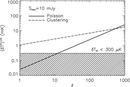
The Poisson and clustered contribution to the sky brightness temperature fluctuations due point sources for a flux cut-off value of Smax = 10 mJy. The brightness temperature fluctuations due to the 21 cm signal is expected to be ≲ 300 μK at redshifts z ≈ 0.5 and is indicated by the hatched region.
The total contribution to δTps is then the quadrature sum of the Poisson and clustered components (they are uncorrelated), i.e. |$C_{\ell }^{\rm ps} = C_{\ell }^{\rm Poisson} + C_{\ell }^{\rm clustering}$| which leads to |$\delta T_{\rm ps}=\sqrt{\delta T_{\rm Poisson}^2 + \delta T_{\rm cluster}^2} =10.6$| mK. We note that there is considerable uncertainty in this estimate, particularly with the clustered component. The extrapolation of our source count into the low flux density (≪0.1 mJy) regime may be unreliable (e.g. because the ARCADE results may imply an unexpectedly large population of very weak sources) and can only be firmly established by ultradeep radio surveys with upcoming telescopes (e.g. Norris et al. 2011). Nonetheless, we believe our calculation suggests that the, often neglected, clustered component is at least as large as that from Poisson fluctuations.
Other foregrounds
A number of other foregrounds could also contribute to Tsky. Other diffuse continuum emission mechanisms include thermal dust and spinning dust emissions. Both of these are expected to be negligible at ν ∼ 1 GHz. For example, extrapolation of the thermal dust model of Finkbeiner et al. (1999), at 1° resolution predicts δT ∼ 2 × 10⁻⁶ mK for |b| > 30°. Similarly, extrapolating the anomalous microwave emission observed at 23 GHz by Wilkinson Microwave Anisotropy Probe (WMAP; Davies et al. 2006) and assuming that it is all due to spinning dust emission from the cold neutral medium (CNM; Draine & Lazarian 1998), gives δT ∼ 2 × 10⁻³ mK and can therefore be safely neglected.
THE BINGO CONCEPT
The discussion presented in Section 3 suggests that in order to get a good detection of BAO at low redshifts (case A from the optimization study) a suitable single telescope should satisfy the following design constraints:
an angular resolution defined by θFWHM ≈ 40 arcmin corresponding to an underilluminated primary reflector with an edge taper <−20 dB;
operate in the frequency range above 960 MHz with a bandwidth that is as wide as possible – exactly how wide and exactly where the band is positioned will ultimately be determined by those parts of the spectrum relatively free of radio frequency interference (RFI);
frequency resolution should be ∼1 MHz or better;
frequency baseline should be as free as possible from instrumental ripples, particularly standing waves (Rohlfs & Wilson 2004);
the receivers should be exceptionally stable in order to allow thermal-noise-limited integrations of a total duration long enough to reach a surface brightness limit ∼ 100 μK per pixel;
the sky coverage as large as possible, but at the very least >2000 deg2 with a minimum size in the smallest dimension of 10°;
the number of feeds7 should be nF > 50 in order to achieve a sufficiently large signal-to-noise ratio;
sidelobe levels as low as possible so as to minimize the pickup of RFI and emission from strong sources; and
beam ellipticity <0.1 in order to allow map-making and power spectrum analysis routines to work efficiently.
For reasons of stability, simplicity and cost, a telescope with no moving parts would be very desirable. We suggest that the following conceptual design could deliver what is required. We first concentrate on the telescope and then on the receiver design. We have named the overall project BINGO.
The telescope and focal plane
Operation at frequencies between 960 and 1260 MHz is a practical possibility because it avoids strong RFI from mobile phone down-links which occupy the band up to 960 MHz. In order to achieve the desired resolution (better than 40 arcmin at 1 GHz), an underilluminated primary reflector of about 40 m projected aperture diameter, D, is required.8 If the telescope is to have no moving parts, i.e. fixed pointing relative to the ground, then a wide instantaneous field of view (FOV) with multiple feeds is essential so that as the Earth rotates a broad strip of sky can be mapped during the course of a day. To reach the target sensitivity, a minimum number of 50 pixels is required in the focal plane, each of them reaching the following performance.
Forward gain–loss in comparison to central pixel <1 dB.
Cross-polarization better than −30 dB.
Beam ellipticity lower than about 0.1.
We propose to adopt an offset parabolic design in order to avoid blockage, minimize diffraction and scattering from the struts, and also to avoid standing waves that might be created between the dish and the feeds. A wide FOV with the required optical performance mentioned above can only be achieved with a long focal length. We found that a focal length F = 90 m, giving a focal ratio F/D = 2.3, much larger than more conventional radio telescopes (having typically a F/D ratio of about 0.4), is suitable for our purpose. This has the drawback of requiring the use of feeds with a small full width at half-maximum (FWHM), therefore with a large aperture diameter. For our telescope design, this means feeds with an aperture diameter of at least 2 m producing an edge taper telescope illumination of −20 dB in order to reduce the spillover. We are targeting a spillover of less than 2 per cent in total power as the fraction of the horn beam not intercepting the telescope will see radiation from the ground therefore increasing the system temperature Tsys.
The design adopted for the focal plane is given in Fig. 16. A line of eight feeds allows for coverage of a 10° strip. Along the scanning direction produced by the Earth's rotation, other lines of feeds are staggered to allow for a proper sampling on the sky. With this configuration, 60 pixels, 10 more than the requirement, will produce a 10 × 9 deg2 FOV. Assuming a feed aperture diameter of about 2 m, the resulting focal plane will be comprised within a rectangle of 16 m × 15m.
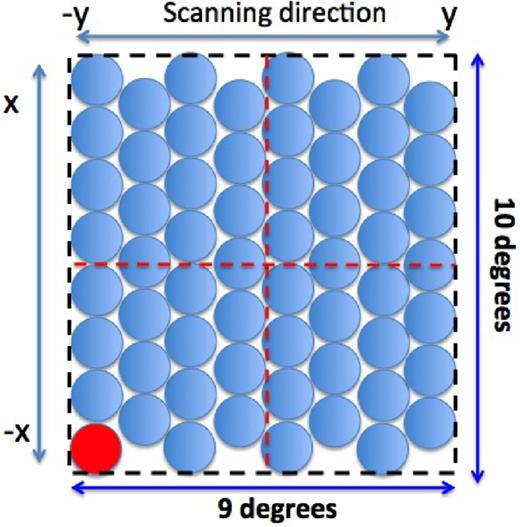
Focal plane of staggered feeds. A total of 60 pixels laid out in a rectangle (dashed black line) of 16 m × 15 m. This will allow for a FOV of about 10 × 9 deg2. Axes x and y are shown as a reference to the positions mentioned in Table 4. The pixel shown in red is the off-axis pixel corresponding to the beam profiles in Fig. 17.
Optical simulations of such a concept have been performed using Physical Optics (GRASP from ticra) in order to take into account the diffraction effects. Results from this model, assuming ideal components (perfect telescope and Gaussian feedhorns) and a perfect alignment, are given in Table 4. The performance is well within the requirements even for the most off-axis pixel (represented in red in Fig. 16). Fig. 17 represents the modelled contour plot of the beams (co- and cross-polarization beams) in the U–V plane that can be expected for the pixel located at the corner edge of the focal plane. Taking into account degradations due to using real components and with typical alignment errors, we can still expect to meet the requirements.
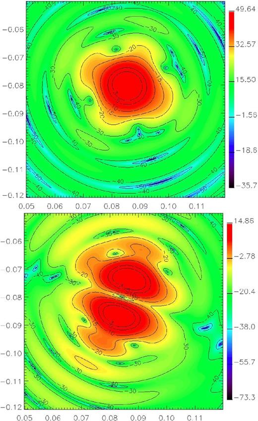
U–V maps of beam intensity for the most off-axis pixel corresponding to the focal plane position x = −8m and y = −7.5 m (represented in red in Fig 16). Top: copolarization; bottom: cross-polarization. Simulations performed using ideal telescope and horn. The coordinates are measured in radians. Colour scale: the gain in dB relative to maximum.
Optical performance calculated using GRASP assuming ideal telescope and Gaussian feeds with −20 dB edge taper. Results are given for a pixel that would be located at the centre of the focal plane and for the corner edge pixel (red in Fig. 16 at x = −8 m; y = −7.5 m). Peak cross-polarization is given, respectively, to the copolarization forward gain.
| Pixel | Forward | Ellipticity | Peak | FWHM |
|---|---|---|---|---|
| position | gain | X-Pol | ||
| (dB) | (dB) | (arcmin) | ||
| Centre | 49.8 | 10−3 | −40 | 38 |
| Edge | 49.6 | 0.07 | −35 | 39 |
| Pixel | Forward | Ellipticity | Peak | FWHM |
|---|---|---|---|---|
| position | gain | X-Pol | ||
| (dB) | (dB) | (arcmin) | ||
| Centre | 49.8 | 10−3 | −40 | 38 |
| Edge | 49.6 | 0.07 | −35 | 39 |
The design concept is illustrated in Fig. 18 and the key parameters are listed in Table 5. Rather than a high tower to support the focal arrangement, the plan would be to identify a suitable site in which the dish structure can be built below a cliff (or near vertical slope) of height 90 m so that the feed arrangement can be fixed on a boom near the top of the cliff.
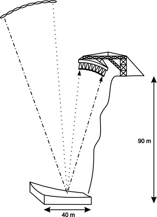
Schematic of the proposed design of the BINGO telescope. There will be an underilluminated ∼40 m static parabolic reflector at the bottom of a cliff which is around ∼90 m high. At the top of the cliff will be placed a boom on which the receiver system of 60 feedhorns will be mounted.
Summary of proposed BINGO telescope parameters.
| Reflector diameter | 40 m |
|---|---|
| Resolution (at λ = 30 cm) | 40 arcmin |
| Number of feeds | 60 |
| Instantaneous FOV | 10° × 9° |
| Frequency range | 960 MHz to 1260 MHz |
| Number of frequency channels | ≥ 300 |
| Reflector diameter | 40 m |
|---|---|
| Resolution (at λ = 30 cm) | 40 arcmin |
| Number of feeds | 60 |
| Instantaneous FOV | 10° × 9° |
| Frequency range | 960 MHz to 1260 MHz |
| Number of frequency channels | ≥ 300 |
Design for a receiver module
A high degree of stability is an essential design criterion both for telescope and receivers. Such demands are not unique since instruments used to measure the structure in the CMB have been built which meet similar stability criteria. In CMB experiments, correlation receivers (or interferometers) are generally the design of choice (e.g., WMAP and Planck). They can reduce the effect of gain fluctuations in the amplifiers (1/f noise) by up to three orders of magnitude (Mennella et al. 2010).
We plan to adopt the same approach with each receiver module producing a ‘difference spectrum’ between the desired region of sky and a reference signal. The choice of the reference is important. Ideally, it should have the same spectrum as the sky and be close to the same brightness temperature. It must also be very stable. An obvious choice is another part of the sky. We propose that there should be a reference antenna for each module with a beam width of around 20° which would have a beam area sufficiently large to average out all but the lowest ℓ modes (see Fig. 2). It should be fixed and we suggest that it should point directly to one of the celestial poles. In this way, all measurements at all times of day, and all the year round, would then be compared to the same region of sky. Since the sky emission has significant linear polarization (∼10 per cent or more; Wolleben et al. 2006), measuring with circularly polarized feeds is necessary. Similar considerations will be important for foreground emission removal. A schematic diagram for a single polarization channel of the proposed receiver module design is shown in Fig. 19.
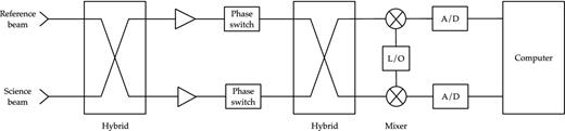
Block diagram of the receiver chain. The reference beam will point towards one of the celestial poles. The hybrids will be waveguide magic tees. After the second hybrid the signal will be down-converted using mixers with a common local oscillator. There will be further amplification before digitization.
Receiver simulations
An ideal correlation receiver – one with perfectly matched system temperatures and no imbalance in the power splitting within each hybrid – can effectively remove all 1/f noise from its signal output. If A = Asys + δA and B = Bsys + δB are the total voltages entering the receiver chain and |$\scriptstyle{A_{\rm sys}\propto \sqrt{T_{\rm sys}^A}}$| and |$\scriptstyle{B_{\rm sys}\propto \sqrt{T_{\rm sys}^B}}$| are the system temperature contributions and δA and δB are the signals we want to detect, then the difference detected power at the end of the chain is proportional to the difference, δA2 − δB2, between the science (A) and reference beam (B). The spectrum of such a signal exhibits no excess power at low frequencies (1/f noise) as illustrated in Fig. 20(a), and integration can continue indefinitely with the white noise falling as the square root of integration time.
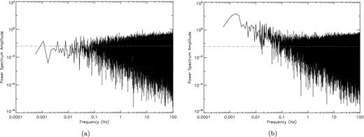
Simulated noise power spectra for a realistic BINGO receiver which uses amplifiers with fknee = 1 Hz and a 30 min integration. Here, (a) represents a perfectly balanced receiver; and (b) a receiver with imbalances in both system temperature (Asys − Bsys)/Asys = 0.2 and power splitting, ϵ = 0.4. These values are significantly larger than expected in a realistic situation and have been chosen to illustrate the point. The upturn of the spectrum in (b) indicates the presence of 1/f noise.
However, real life receivers are imperfect. Imbalances between system temperature and power splitting both limit the reduction of the 1/f noise resulting in a break in the power spectrum quantified in terms of a knee frequency (Seiffert et al. 2002) separating white noise-dominated and pink noise-dominated parts of the spectrum. Consequently, there will be a limit to the viable integration time as illustrated in Fig. 20(b). It is useful to quantify by how much a correlation receiver is limited by these imperfections, and to do so we simulate their effect in a realistic receiver model. We assess the maximum permissible imperfection amplitude to ensure that the knee frequency remains below fknee ∼ 1 mHz, a value corresponding ∼20 min integration time – sufficient for the largest H i structures we are interested in detecting, ∼a few degrees, to drift through the telescope beam.
We include Gaussian (white) and 1/f noise, generating the former using a simple random number procedure and the latter with a more complex auto-regressive approach – essentially filtering a white noise time stream into one with correct correlation properties. The knee frequency of component amplifiers depends on both the physical choice of amplifier and the channel bandwidth. Though the actual value will need to be determined empirically, we will assume in the current simulations that the individual amplifier knee frequencies are |$f_\mathrm{knee}^\mathrm{amp}\sim 1\,{\rm Hz}$| for a channel bandwidth of 1 MHz.
Unbalanced Tsys
In an ideal receiver the two channels, Asys and Bsys, should be perfectly matched. This is impossible to achieve at all times due to the angular variations in the Galactic emission and here we investigate the effect on the knee frequency due to small imbalances between the temperatures.
Modelling the entire correlation receiver and simulating noise spectra for the output difference signal in the presence of small temperature imbalances, we find that the knee frequency of the correlation receiver can be approximated by fknee = 1.2 Hz ((Asys − Bsys)/Asys)2 and therefore to ensure that BINGO's knee frequency remains continually below the desired fknee ∼ 1 mHz, our simulations show that (Asys − Bsys)/Asys needs to be <0.03. In practice, the balance can be maintained electronically so this should not be an important limitation, provided the unbalance behaves predictably as a function of time. The main source of imbalance in the system temperatures will arise from the changing sky background as the telescope scans across the sky. Typical variations in those parts of the sky of interest well away from the Galactic plane will be a few Kelvin and will be repeatable from day to day. Importantly, the sky emission will be spectrally smooth and virtually identical in all frequency channels. This means that once the frequency-averaged variation of sky brightness has been measured over the course of a siderial day, a multiplicative correction, the r-factor defined by Seiffert et al. (2002) can be applied to all channels to bring the A and B outputs into balance before differencing, thus ensuring the (Asys − Bsys)/Asys < 0.03 is met.
Power split imbalance
Here, we assume the power splitting imbalances in the first and second hybrids are equal, and simulate noise spectra for different values of ϵ. Fitting for the knee frequency we find fknee = 4ϵ2 Hz. Again, in order to maintain a knee frequency of 1 mHz, this relationship implies that the power splitting imbalance should satisfy ϵ < 0.015. This requirement can be relaxed if a 180° phase switch is used within the hybrid loop and, since waveguide magic tees typically have a power split imbalance of ϵ = 0.02, the required performance should be achievable.
Practicalities
Our philosophy is to choose simplicity while keeping in mind good engineering practice and, wherever possible, to adopt conventional solutions to problems rather than try to invent new ones.
To reduce the impact of RFI the telescope would need to be in a remote site and therefore an important additional consideration is that everything should be easy to maintain. The design, construction and mounting of the feeds are perhaps the most challenging aspects of the overall concept. As stated above, low sidelobe levels are important in order to mitigate the effects of RFI (even in the remotest part of the world) and ease the separation of foreground emission from the desired neutral hydrogen signal. If a conventional horn design is adopted, these horns will have to be extremely large; to illuminate a 30 m dish from a focus ∼75 m away will require an aperture diameter for each feed of 1.5 to 2 m and a length of ∼8 m. Such feeds are practical, in the sense that they would be scaled up versions of horns built to existing feed designs, but could prove expensive to build and unwieldy. Alternatives like using small secondary mirrors for each receiver module are under consideration.
An integral part of the feed system is the extraction of polarized signals which we will do by extracting the two opposite circular polarizations. Minimizing any Ohmic loss before the first amplifiers is essential if good thermal noise performance is to be achieved. After the feed the next element is the hybrid. Due to their low loss and good power splitting properties we would use waveguide magic tees.
We would use non-cryogenic LNAs because at this frequency the noise advantages of cooling to ∼20 K are outweighed by the low cost, the low power consumption and the low maintenance demands of a non-cryogenic approach. It would also be desirable to integrate the amplifiers with the magic tee to avoid the necessity to use potentially lossy cables. Some cooling, perhaps using Peltier coolers, could be used because it would provide both temperature stabilization for the amplifiers and a potential improvement in noise performance.
An important choice is when to digitize the signal. In conventional correlation receivers the ‘correlation’ is performed in a second hybrid. Our preferred solution is to down-convert the radio frequency signal with a common local oscillator and then to digitize and perform the function of the second hybrid in software using FPGAs to multiply the signals and produce averaged spectra which can then be differenced. One advantage of such a system is that the levels in the two arms of the receiver can be easily adjusted so that they are the same and this then operates the receiver at its optimum for gain fluctuation reduction.
CONCLUSIONS
Intensity mapping is an innovative idea which has been suggested to allow LSS surveys using the 21 cm line of neutral hydrogen using instruments with relatively small collecting area compared to the SKA. Such concepts would naturally be much cheaper. We have presented calculations that illustrate the characteristics of the signal and it is shown that it should have an rms of ∼ 100 μK on angular scales ∼1° and bandwidths of 1-10 MHz. At very low redshifts there will be a shot noise effect due to it being dominated by individual galaxies, at medium redshifts it is dominated by the effects of H i in galaxy clusters and at high redshifts becomes an unresolved background.
We have performed an optimization analysis which suggests that a significant measurement of the acoustic scale can be made between z = 0.13 and 0.48 using a single dish telescope of diameter 40 m with a drift scan survey of a strip with width 10° covering a total of ∼2000 deg2. In order to do this at higher redshift (specifically, the case of z = 0.58 − 1.47) would require a much larger dish, ∼140 m, and an area of 500 deg2 which would probably be best done using an interferometer in order to allow non-drift scan observations using such a long baseline instrument. We have presented a detailed assessment of the likely foregrounds and conclude that there will be continuum fluctuations with an rms of ∼100 mK on degree scale, but that this should not significantly affect our ability to extract the H i signal due to the fact that its spectral profile is expected to be relatively smooth.
We have put forward a design concept, which we have named BINGO, to perform the lower of the two redshift surveys studied. This will use a large focal length telescope, F/D ≈ 2.3, to mount an array of 60 feedhorns approximately 90 m above a static 40 m. It will use pseudo-correlation receivers to reduce 1/f noise due to gain fluctuations. We are currently searching for a site and the funding needed to bring this idea to fruition.
We thank Peter Dewdney for suggesting the use of a cliff to mount the BINGO feeds and Xiang-Ping Wu for suggesting using one of the celestial poles as a reference. We have had numerous useful discussions with Peter Wilkinson, Shude Mao and Richard Davis. CD acknowledges an STFC Advanced Fellowship and an EC IRG grant under the FP7. AP is supported by the project GLENCO, funded under the FP7, Ideas, Grant Agreement no. 259349 and also received support from the STFC (UK). We thank Bob Watson for help in creating Fig. 18. Finally, we thank the referee for a number of helpful comments which have improved the paper and also were very helpful in developing the details of the BINGO design.
We note that this might be different if we had chosen another science goal such as the measurement of neutrino masses.
We note that varying Ωmh2 modifies dV(z) and the present limits on this parameter combination are included in Fig. 11. These will be substantially improved in the next couple of years.
For convenience we refer to extragalactic sources as a foreground though both lower redshift (foreground) and higher redshift (background) sources will contaminate the H i signal.
We will use a conventional feedhorn array. An alternative would be to use a phased array feed. However, at this stage we do not judge that such technology is sufficiently well developed to fit with our philosophy of simplicity.
The equivalent fully illuminated aperture would be D ≈ 25 m.
