


Abstract
The standard visibility model in light-pollution studies is the formula of Hecht, as used e.g. by Schaefer. However, it is applicable only to point sources and is shown to be of limited accuracy. A new visibility model is presented for uniform achromatic targets of any size against background luminances ranging from zero to full daylight, produced by a systematic procedure applicable to any appropriate data set (e.g. Blackwell's), and based on a simple but previously unrecognized empirical relation between contrast threshold and adaptation luminance. The scotopic luminance correction for variable spectral radiance (colour index) is calculated. For point sources, the model is more accurate than Hecht's formula and is verified using telescopic data collected at Mount Wilson in 1947, enabling the sky brightness at that time to be determined. The result is darker than the calculation by Garstang, implying that light pollution grew more rapidly in subsequent decades than has been supposed. The model is applied to the nebular observations of William Herschel, enabling his visual performance to be quantified. Proposals are made regarding sky quality indicators for public use.
1 INTRODUCTION
1.1 Contrast threshold
Determining the faintest star or extended object visible to the naked eye or with a telescope is a problem of interest in light-pollution studies, the history of astronomy and vision science. It is an issue of public concern and economic importance given the growth of recreational ‘dark-sky parks’ for amateur astronomy and the imposition of lighting ordinances to preserve the aesthetic quality of the night sky (IDA 2013). This paper will present a model applicable to uniform achromatic targets of any size, seen against background luminance levels ranging from total darkness to daylight, hence relevant to visibility problems in many areas. For low light levels, it will be applied to historical astronomical data and shown to be more accurate than previous models.
1.2 Blackwell's data
The largest and most authoritative study of contrast threshold was that of Blackwell (1946), whose data continue to be used in areas such as lighting engineering and road safety (Narisada & Schreuder 2004). They were used in a popular book for amateur astronomers by Clark (1990) to make graphical predictions of astronomical visibility. The approach to be taken here is instead analytic, giving rise to formulae relevant to a wide range of visibility problems, and applicable to data other than Blackwell's. Blackwell measured luminance in footlamberts, but the data will be presented here in modern units (1 fL = 3.426 cd m−2). Blackwell investigated both positive and negative contrasts, but only the positive data (target brighter than surround) will be considered in this paper.
In order that the data can be correctly interpreted, it is necessary to consider the experimental method in some detail. A total of 19 highly trained female observers aged 19–26 with approximately 20/20 vision were employed specially for the project (serving also as data analysts). No gender effect has been reported in the literature, but the age, experience and motivation of the observers is significant. Observers viewed targets using unconstrained (direct or averted) binocular vision for effectively infinite time (i.e. such that doubling of exposure did not alter successful detection rates). Targets viewed at effectively infinite range (over 15 m) were uniform achromatic (broad-band white) discs of seven angular sizes ranging from 0.595 arcmin to 6°. These were either projected or, for the smallest target, transilluminated. They were viewed against backgrounds ranging from 3426 cd m−2 down to zero, and at five levels of contrast (in relative proportion 0.24, 0.37, 0.55, 0.75, 1). Observers were always allowed to become fully adapted to the background luminance, and rest periods were given so as to avoid fatigue. A single session would consist of 320 presentations, and observers were not considered trained until they had participated in approximately 20 sessions, though the published data were based on a far higher level of experience (35–75 000 observations by each observer) resulting in ‘unusual sensitivity and gratifying stability of response’.
For every target and contrast level, each observer's probability of detection was found. For each observer's probability curve (approximately a normal ogive), a graphical procedure was used to extract the contrast value M that would correspond to 50 per cent detection, chosen since it could be calculated with highest precision, and σ, the standard deviation of the normal probability integral. Results from 1500 probability curves were averaged, giving contrast threshold as a discrete function of target size and background luminance: table 7 of Blackwell (1946) summarizes 90 000 observations by seven observers. Smooth curves were drawn as a best fit to these data points, and interpolations made, to produce the final values (table 8 of Blackwell 1946).
At ordinary light levels (for discs larger than 0.595 arcmin), a ‘forced-choice’ procedure was used, in which the target would appear in one of eight possible positions (or not at all), and observers had to indicate where they thought the target was displayed using a selector switch at the end of the viewing period. At low light levels, requiring much longer viewing times, a two-valued forced-choice procedure was used (‘yes–no’), in which the target was presented (or not) at the centre of the screen, and observers had to indicate whether they had seen it, again with a switch. Null targets enabled the effect of random guessing to be eliminated.
The 50 per cent detection level was merely a statistical normalization: the threshold at any other detection probability p could be found by applying a multiplier f = 1 + (σ/M)z, where z is the normal distribution standard score for cumulative probability p (Blackwell 1952a). It is interpreted as meaning that an observer, exposed many times to a threshold target under the conditions of the experiment, would be expected to respond correctly on 50 per cent of occasions. It does not mean that during a single observation the target should be visible for 50 per cent of the time, as suggested by Clark (1994): an observer able to see the target for any period of time during every exposure would be expected to achieve a success rate of 100 per cent (assuming no mistaken responses or false positives). Nor does it mean that the observer would be 50 per cent confident of having seen the target, as supposed by Schaefer (1990). Blackwell reported that, in general, observers were confident of having seen the target only in cases where the resulting detection probability was 90 per cent or greater, corresponding to f = 1.62, suggesting that thresholds should be multiplied by at least this much to give realistic values. Blackwell & Blackwell (1971) noted that subjects in forced-choice experiments could show a detection rate slightly better than chance, even when not consciously aware of having seen the target. Higher (poorer) thresholds are found if observers instead adjust the brightness until the target becomes just visible. In order to raise forced-choice thresholds to what they termed ‘common-sense seeing’, Blackwell & Blackwell proposed a multiplier 2.4. The application of an overall multiplier to laboratory data will here be termed ‘laboratory scaling’, and can be used as a way of comparing data from studies performed under different experimental conditions.
Blackwell's data were extended to larger target sizes by Taylor (1960a,b), and to all observer ages by Blackwell & Blackwell (1971). Threshold was found to rise with increasing age: slowly up to about 45, then quite rapidly. This is due mainly to loss of transparency in the ocular media (Adrian 1989) rather than diminution of pupil size, as assumed by Schaefer (1990). However, it was found that to a very good approximation, the shape of the threshold curve (on log axes) remained invariant, i.e. the effect of age is to introduce a further overall multiplier, in addition to laboratory scaling. Empirically determined age multipliers in Blackwell & Blackwell (1971) range from 1 for 50 per cent of 20-yr-olds, to 6.92 to include 95 per cent of 65-yr-olds.
The age multiplier is an example of a ‘field factor’ (Taylor 1964) constituting a departure from the laboratory conditions. More generally, these may be associated with the target (e.g. non-circular shape, non-uniformity), viewing conditions (non-uniform background, glare sources) and observer (motivation, fatigue). The field factors contribute further multipliers to the contrast threshold. There may also be physical effects which objectively alter the stimulus, such as magnification or light loss in a telescope, needing to be taken into account as A → A′, B → B′. Hence in practice the threshold function is FC(A′, B′), where F – the product of all field factors and any laboratory scaling – has the effect of shifting the whole curve up or down on log axes. Thus, the threshold function should in general be considered relative rather than absolute (Blackwell 1952b), but invariant in shape, implying a correlation between threshold at large and small target sizes (i.e. in astronomy, an equivalence between limiting stellar magnitude and limiting surface brightness).
This suggests two approaches to visibility modelling. One (here called ‘enumeration’) is to attempt to quantify all the relevant field factors from physical data (or estimate them) and hence determine F for a given observing situation. The other (‘elimination’) is to leave F as an unknown variable, unless data are available that allow it to be determined, or calculations can be performed where it cancels out. Schaefer (1990) studied stellar visibility using enumeration, whereas this paper will treat targets of arbitrary size using elimination. Schaefer assumed that the personal factor of the observer (which he denoted Fs) was approximately 1, but that the detection probability could vary, whereas actually the latter is a fixed normalization constant and the personal factor may vary considerably between individuals. The error was mathematically insignificant since the threshold is multiplied by the product of these factors.
1.3 Photometric considerations
If the v-magnitude scale has zero-point Zv lx, then J lx is equivalent to apparent magnitude mv = 2.5 log(Zv/J), and B cd m−2 is equivalent to surface brightness |$\mu _v= 2.5\,\rm{log}(60^{4}(180/\pi )^{2}Z_v/B)\;\rm{mag}_v$| arcsec−2. Taking ZV = 2.54 × 10⁻⁶ lx (Cox 1999) gives conversion formulae mV = −2.5 logJ − 13.99, μV = −2.5 logB + 12.58. Henceforth, magnitude can be assumed to be V-band unless indicated otherwise.
The darkest skies on Earth have a zenith luminance of approximately 22 mag arcsec−2 (1.71 × 10⁻⁴ cd m−2), with the visible sky background on a clear moon-less night being a combination (in descending order) of natural airglow, zodiacal light and unresolved starlight (Leinert et al. 1998). Airglow typically accounts for about 60 per cent of zenith sky luminance (Leinert et al. 1995), varying with solar activity, and dominated by the 557.7 nm O i emission line which alone typically contributes around 20 per cent of total V-band sky brightness (Patat 2008). At urban sites, the sky spectrum is dominated by tropospheric scattering of anthropogenic light; measurements by Puschnig, Posch & Uttenthaler (2014) near Vienna showed very large peaks at 546 and 611 nm (attributable to fluorescent street lamps) with smaller intervening peaks due to high-pressure sodium lamps. Zenith sky brightness was in the range 15–19.25 magSQ arcsec−2 (approximately 1.1 × 10⁻¹–2.2 × 10⁻³ cd m−2). As a general approximation, one can take 2 × 10⁻⁴ cd m−2 (21.83 mag arcsec−2) as representative of a truly dark sky, though at a pristine site there may be regions of the sky that are darker than this (Duriscoe 2013).
Human vision at normal light levels is photopic, utilizing the trichromatic cone cells whose density is greatest in the foveal region of the retina. In very low light levels vision is scotopic, utilizing the monochromatic rod cells whose density is greatest outside the fovea. There was formerly thought to be an abrupt switch between the two types of vision, though in fact, there is a continuous transition at intermediate (mesopic) light levels as cone response lessens and rods become active. Hence, it is misleading to speak of ‘day’ and ‘night’ vision. The transition is dependent on the particular visual task and prevailing conditions, so cannot be specified exactly, but as a working definition one can take the range of mesopic vision as 0.005–5 cd m−2 (CIE 2010), i.e. scotopic vision operates in conditions darker than about 18.3 mag arcsec−2. For astronomical purposes, Puschnig et al. (2014) estimated the limit as 18.9 magSQ arcsec−2 (approximately 0.003 cd m−2).
Vision has ‘channels’ for luminance and chromaticity; contrast can be defined with respect to either, but in scotopic vision only the luminance channel operates. If an observer is able to detect colour then this indicates cone activity, so nocturnal astronomical observation often involves mesopic rather than scotopic vision. Variable star observers generally restrict magnitude estimates to stars at least 2 mag brighter than threshold, using direct rather than averted vision, which gives more reliable estimates since it minimizes rod contribution (Hallett 1998). Schaefer (1996) found from a survey of experienced observers that in telescopic stellar viewing, scotopic vision operates at no more than about 1 mag above threshold. Mesopic photometry would be important for a proper treatment of suprathreshold magnitude estimates or visibility under severe light pollution (including twilight). However, this paper is concerned with threshold rather than brightness perception; and although the model will cover achromatic vision across the entire luminance range, the astronomical applications will be restricted to scotopic vision, i.e. targets within about 1 mag of threshold against a background no brighter than about 3 × 10⁻³ cd m−2 (18.9 mag arcsec−2), to which the observer is assumed fully adapted.
The spectral radiance of the sky is variable: at a given site there will, for example, be temporal changes in airglow, variation of tropospheric scattering with zenith distance, and variation of zodiacal light with ecliptic latitude. Zodiacal light is scattered sunlight, and its spectrum is almost identical to the Sun's at visible wavelengths (fig. 38 of Leinert et al. 1998); integrated starlight has approximately the same spectrum over that range (fig. 1 of Leinert et al. 1998). Hence, the moon-less zenith sky without light pollution can reasonably be approximated by a 5500 K blackbody spectrum together with airglow lines in some relative percentage of luminance. Taking the typical airglow spectral data given in table 13 of Leinert et al. (1998), one finds ρsky ranging from 0.79 (100 per cent airglow) to 2.26 (0 per cent), with a typical figure (60 per cent) being 1.38. This is very close to the S/P ratio of Blackwell's light sources (1.41, equivalent to 58 per cent airglow). It is therefore reasonable to take the spectral radiance of Blackwell's background as a sufficiently good approximation of a typical moon-less night sky in the absence of light pollution.
1.4 The data of Knoll et al.
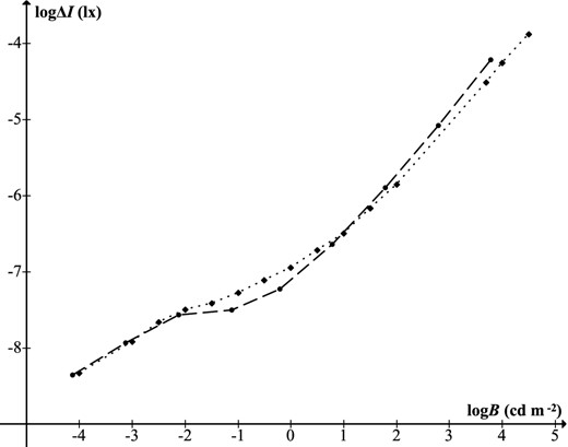
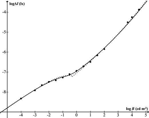
The point-source visibility study of Knoll et al. (1946) is of special interest because of its role in subsequent astronomical applications. Five young experienced observers used binocular vision to view a projected target of approximate diameter 1 arcmin. Each observer was given unlimited time to raise and lower the target brightness to find the level at which it was just visible. Thresholds were presented as equivalent increments (ΔI) for an opaque target. To compare the results with the point-source thresholds of Blackwell (1946), the latter's scotopic luminance values (for background and increment) must be multiplied by 1.220 because of the differing colour temperatures, and a further overall multiplier, l, must be applied to the increments because the method of adjustment yields higher thresholds than forced choice with 50 per cent detection probability. Tousey & Hulburt (1948) proposed l = 2, because this was close to the Blackwell normalization multiplier f for forced-choice detection probability close to 100 per cent, though in the adjustment procedure, the concept of detection probability is strictly meaningless. In fact, one finds that l = 1.814 brings the scotopic data (−4 ≤ logB ≤ −2) into almost exact agreement (Fig. 1). Adjustment would also be required at mesopic levels, though some discrepancy would likely remain (as also at photopic levels), attributable to the differing experimental procedures, though not relevant to the astronomical situations considered in this paper. For scotopic point-source thresholds (i.e. stars at night) the two data sets are effectively equivalent, though Blackwell's data are to be preferred as the more authoritative.
1.5 Visibility models
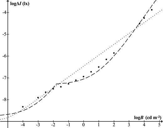
While it has long been appreciated that Hecht's photochemical theory was invalid (Westheimer 1999), and that there is not really a discontinuous break between photopic and scotopic vision, what has not been noticed is that for the luminance range relevant to astronomical observation, Hecht's formula was actually inferior to the one by Knoll et al. which it was supposed to replace. Fig. 2 shows the mean data from Knoll et al. (1946) converted to modern units, together with equations (19) and (20). An equivalent graph was presented in the original units by Hecht (1947). While it is evident that Hecht's model is greatly superior for photopic vision, it can be seen that this is not so in the scotopic (and lower mesopic) region. For logB in the range −1.5 to −4 (16.33–22.58 mag arcsec−2), the data form a compressive curve whereas Hecht's curve is accelerating. The straight line of Knoll et al. is better, but the new model presented here will be seen to be of the correct shape, providing a more accurate estimate of stellar visibility.
1.6 Astronomical visibility factors
1.6.1 Viewing time
Astronomical observations are often enhanced by long viewing times; Clark (1994) cited O'Meara's visual recovery of Halley's comet after 1–2h, claiming it demonstrated a long-term integration property of the visual system. However, saccades limit fixation time to no more than about a second, comparable with the maximum integration time of retinal cells. Bishop & Lane (2004) measured the shortest viewing times such that telescopic targets appeared undimmed compared with unlimited exposure, using the 0.61 m telescope at Mauna Kea, and found times of 1.03 s or less. Confusion over Blackwell's definition of detection probability has led to an incorrect assumption that it is related to exposure time (Schaefer 1990); however, laboratory experiments have shown that long viewing times generally degrade rather than enhance performance (Mackworth 1948). The benefit in astronomy can be explained by atmospheric variability; planetary observers are familiar with moments of best seeing, but what is less generally appreciated are fluctuations of transparency.
1.6.2 Atmospheric turbulence
Air turbulence creates variations of refractive index manifested in seeing (image motion caused by tilting of wavefronts) and scintillation (brightness variation caused by curved wavefronts focusing or defocusing starlight; Dravins et al. 1997a). The two effects are distinct, with major contributions from different atmospheric altitudes, and have little or no correlation, though aperture dependence leads to an apparent correlation for naked-eye viewing, i.e. more noticeable scintillation on nights of poor seeing. A site with excellent seeing can nevertheless have high scintillation.
As will be explained in Section 2, at scotopic levels point sources are indistinguishable from extended targets up to about 10 arcmin in diameter. Hence, seeing is important for high-magnification telescopic viewing, but has no effect on naked-eye viewing. Scintillation, on the other hand, has greatest effect for naked-eye viewing, and is of potential significance for threshold determinations with or without optical aid.
Scintillation occurs on multiple temporal scales, at all zenith angles, and can lead to sudden ‘flashes’ with a brightening of 1–2 mag lasting a hundredth of a second, or lesser increase for longer (Ellison & Seddon 1952). The visibility of brief flashes is dependent on their energy in relation to threshold (Blondel & Rey 1911); specific cases would require detailed calculation, but it can be seen that the general effect is that a very faint star may only be seen momentarily during many minutes of observation, and there may on occasion be a sighting of a star considerably fainter than the usual limit. Scintillation alters the colour of stars (Dravins et al. 1997b) and has a differential effect on point versus extended sources (Dravins et al. 1997a). The effect of scintillation is averaged out by long integration times and large apertures, but human vision has a very short integration time and (for naked-eye viewing) a very small aperture, so that variations are potentially large. The phenomenon is caused by high-altitude winds, so proximity to a main jet stream is expected to lead to higher scintillation: Dravins et al. (1998) noted the high rates measured at Mauna Kea and Paranal, and suggested that there would in general be greater scintillation along latitudes ±30°, and minima at the equator and poles.
The effect of seeing on telescopic views is dependent on aperture. The Fried parameter r0 is the critical diameter above which resolving power is limited by the atmosphere rather than by the telescope's own diffraction (Fried 1966). In a sufficiently large telescope, a star produces a blurred disc of speckles (each of which is an Airy disc) with an approximately Gaussian profile. It is customary to quote the seeing θ as the disc's full width at half-maximum (FWHM), though the actual image is larger. Since FWHM = |$2\sigma \sqrt{2\rm{ln}2}$| for a Gaussian standard deviation σ, and since ±3σ will contain 97 per cent of the light of a Gaussian disc, one could take the actual width of the seeing disc as approximately |$3/\sqrt{2{\rm ln}2} = 2.55\theta$|. To contain 100 per cent, one could take ±3.3σ, i.e. 2.80θ. Schaefer (1990) assumed the disc diameter to be equal to the quoted seeing (in his equation 7), which may be true for small telescopes depending on how the seeing has been assessed by the observer. Garstang (2000) made the same assumption in his model, but applied it to large telescopes.
1.6.3 Position, colour, shape, structure
Zenith angle is a determinant of atmospheric extinction and sky brightness (equations 3 and 19 of Schaefer 1990), as well as atmospheric reddening and scintillation. In the method of enumeration one requires absolute values for these, whereas for elimination it is sufficient to require that observations are all made under sufficiently equivalent conditions. Airmass affects point and extended sources slightly differently (see e.g. Duriscoe 2013 and references therein) and this would need to be taken into account if the most precise results were required, but will not be done here.
It has been shown that Blackwell's experiment at scotopic levels can be considered a good representation of 2850 K blackbody sources against a sky with typical airglow and negligible light pollution. Targets with a spectral radiance very different from blackbody (e.g. emission nebulae), or heavily light-polluted sky backgrounds, would require special treatment using the techniques of Section 1.3. If the concern is with finding limiting magnitude by the method of elimination, it is sufficient to assume that stars are all of approximately the same colour index (as was done by Schaefer 1990; Cinzano et al. 2001), though not necessarily a specific value. For stars of specific colour index equation (16) should be used.
Threshold for rectangular targets was investigated by Lamar et al. (1948) who showed that area is a sufficient determinant for aspect ratios up to approximately 7. Hence, the model should be adequate for elliptical targets with apparent eccentricity up to about this figure. Non-uniform targets will be treated approximately: it will be shown that realistic predictions can be made regarding the visibility of galaxies or the seeing discs of stars. The sky itself can be considered uniform in the immediate vicinity of a target, but field stars potentially introduce glare sources, such that a faint target may be invisible because of a brighter star in the vicinity. This glare effect can be treated in a standard way (Adrian 1989) but specific problems of this type will not be considered here.
1.6.4 Telescope use
Light loss in a telescope introduces a differential effect with respect to naked-eye viewing, and constitutes a stimulus modification. Schaefer (1990) assumed transmittance values according to telescope type, but it will be seen that if multiple observations are recorded under suitably controlled conditions (as was done by Bowen 1947), then the transmittance (denoted |$F_\rm{t}^{-1}$|) can be deduced by elimination. Monocular vision through a telescope introduces another differential effect, though this is a modification of threshold rather than stimulus. Lythgoe & Phillips (1938) measured contrast thresholds with left (CL), right (CR) and both eyes (C), finding the approximate relation 1.4C = 0.5(CL + CR). Theoretical considerations suggested that the factor on the left should be |$\sqrt{2}$|, and if threshold is equal in both eyes then this means the monocular threshold is |$\sqrt{2}$| times the binocular value. This is the factor that was assumed by Schaefer (1990, his Fb), though it was included incorrectly as a stimulus modification in his equation 15 (i.e. as a multiplier of B), and this was repeated by Garstang (2000).
Magnification produces an increase of target area and also in most cases reduction of retinal illumination, because the observer effectively views through an artificial pupil (i.e. the exit pupil of the instrument, which is usually smaller than the eye pupil). In some cases, the Stiles–Crawford effect may need to be considered (i.e. the reduction in luminous efficiency of rays entering the eye obliquely). This is significant for photopic (and mesopic) vision, being attributable to directional sensitivity of cone cells, but Flamant & Stiles (1948) found little or no directional sensitivity in rod cells, while Van Loo & Enoch (1975) found a very small effect, but only for rays entering at the periphery of pupils larger than about 5 mm. Hence, they stated that the usual equation for the photopic effect could not be applied, though Schaefer (1990) proposed such an expression (his equation 9) which incorrectly gives a non-zero value for all pupil sizes. In this paper, the effect will be considered negligible.
Telescope use potentially introduces other differential factors relative to naked-eye viewing. Observers may be apt to use near rather than infinite eye focus when looking through an eyepiece, which may alter the effect of any ocular aberration. The telescope itself may suffer from aberration, and will show the viewer a much smaller apparent area of sky, set within a darker surround. There may be a difference of search procedure between naked-eye and telescopic viewing (e.g. finding known stars to assess naked-eye limit, then searching for hitherto unknown ones to assess telescopic limit). If the telescope is undriven then motion may be a factor. These will be assumed part of an overall telescopic field factor whose components can be split into magnification dependent (FM) or independent (FT) terms. If an approximate value is needed, it will be assumed that |$F_\rm{T} = \sqrt{2}$|, i.e. the only significant magnification-independent factor is the correction for monocular vision. FM can be considered to be unity at low magnification in the absence of the Stiles–Crawford effect, but contributions could come from the use of interchangeable eyepieces of differing specification and quality, and at high magnification the point spread function of the eye will be significant (Watson 2013), with an exit pupil of 0.5 mm usually being regarded as the limit below which diffraction in the eye begins to dominate (Jacobs, Bailey & Bulimore 1992). This imposes a maximum useful magnification (Angers 1998), apart from the limitations imposed by seeing. In practice, it should be sufficient to assume FM = 1 up to some magnification beyond which there is no further improvement in threshold.
1.6.5 Definition of threshold
The activities of amateur astronomers can lie anywhere between science and recreational sport. If the latter, then the individual's concern with limiting magnitude may be to maximize it, whereas for science a main interest should be consistency of measurement. Scintillation in particular is a potential bonus from the recreational point of view, though a source of noise for science.
Threshold can be boosted in various ways: Curtis (1901) observed stars through a hole in a black screen (i.e. against a totally dark background) and in this way was able to see one of magnitude 8.3, and possibly one of magnitude 8.9, though his limit for stars seen against the sky was 6.5. Flickering is known to improve threshold (Kelly 1977): a rapidly operating shutter (e.g. a fan) adjusted to the optimum frequency of around 6 Hz, and placed in the line of sight (e.g. within a telescope), would produce some gain of magnitude. O'Meara (1998) found that hyperventilation helped, consistent with the findings of Connolly & Barbur (2009), though excessive oxygen is damaging to the retina (Yamada et al. 1999).
It has always been appreciated that the traditional naked-eye magnitude limit of 6 is merely approximate. Weaver (1947) commented on the magnitude limits of nineteenth-century naked-eye star catalogues, which ranged from 5.7 (Argelander) to 6.7 (Heis). The latter observer was renowned for his visual acuity, and his Atlas Coelestis is unusual in including the galaxy M33 as a naked-eye object (Heis 1872). Gould's Uranometria Argentina had a stated magnitude limit of 7 but modern photometry has shown the actual limit to be 6.5 (Gould 2010). As an example of exceptional eyesight, Weaver cited Meesters’ ability to see stars to 6.9 mag. Weaver's study upheld a value of just over 6 for the typical dark-sky naked-eye limit, yet more recently there has been a substantial raising of achievement and expectation. The Bortle Scale (Bortle 2001) suggests that for a Class 1 (‘excellent’) site, the limiting magnitude should be ‘7.6–8.0 (with effort)’ and for Class 2 (‘typical truly dark site’) 7.1–7.5. Schaefer (1990) reported O'Meara's extraordinary ability to see stars as faint as 8.4 mag against the sky. Apart from unusual acuity or special observing techniques, such high limits may in many cases be explained by scintillation, with momentary glimpses being taken as typical threshold. Subjective estimates may not always be reliable or accurate; the survey by Schaefer (1990) yielded many responses (about half of the total) in which naked-eye limit was given only to the nearest whole number.
It is a matter of policy judgment whether visibility recommendations for the general public should be based on typical or extreme performance. For modelling, one requires a definition that most closely resembles the conditions of the laboratory data (Blackwell's experiment) and is not unduly sensitive to local effects or false positives. Probably, the best way to achieve this in practice is the method of star counting, using designated areas close to zenith. Stars should be continuously visible (with direct or averted vision) for some extended period (seconds) rather than be seen to flash momentarily. The observer should be fully dark adapted, with screening from terrestrial glare if necessary, and with a naked-eye view of the sky that is at least as large as a typical apparent field of view in a telescope (e.g. 50°). For telescopic views, the use of magnitude sequences (as described by Schaefer 1990) is convenient, but should be consistent with naked-eye procedures. It will be implicitly assumed in subsequent discussion that thresholds effectively conform to these or similar criteria.
2 THE VISIBILITY MODEL
2.1 Modelling strategy
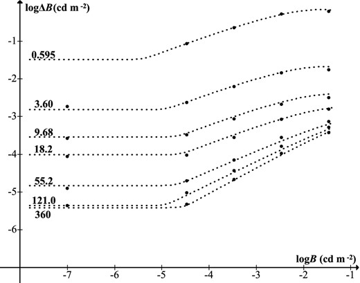
Fig. 3 shows logΔB as a function of logB for various target sizes, using Blackwell's data. In daylight conditions, the slope is approximately 1, i.e. C = constant, which is Weber's law. For extremely low B, the slope of the graph is zero, where ΔB has a non-zero limiting value attributable to neural noise (‘dark light’). The curves indicate that a background B ≲ 10− 5 cd m−2 (25.08 mag arcsec−2) is effectively zero for human vision, a finding also made by Crawford (1937).
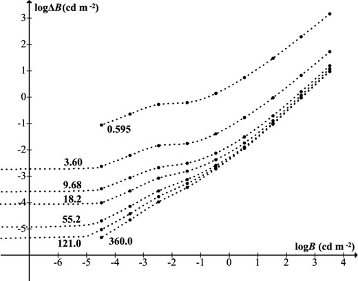
Threshold increment versus background luminance for various target diameters (in arcmin). Data from tables 4 and 8 of Blackwell (1946).
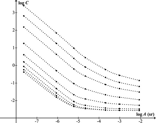
Contrast threshold for different values of background luminance B, from table 8 of Blackwell (1946). Curves are at intervals of 1 log unit, from 3.426 × 10⁻⁵ cd m−2 (top) to 3.426 × 10³ cd m−2 (bottom).
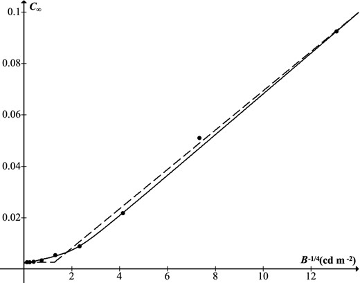
The approach to be taken here is new, and is based on the surprising finding that R and C∞ are both simple functions of B−1/4, across appropriate ranges of B. Model parameters are then specified by linear relations, in a systematic procedure that can be applied to any appropriate data set. The complete function will be C = (Clowq + Chighq)1/q, where q is the only tuneable parameter in the model.
2.2 Point-source model
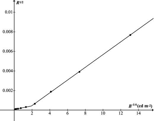
|$\sqrt{R} = \sqrt{CA}$| versus B−1/4, using data from table 8 of Blackwell (1946) for target diameter 0.595 arcmin.
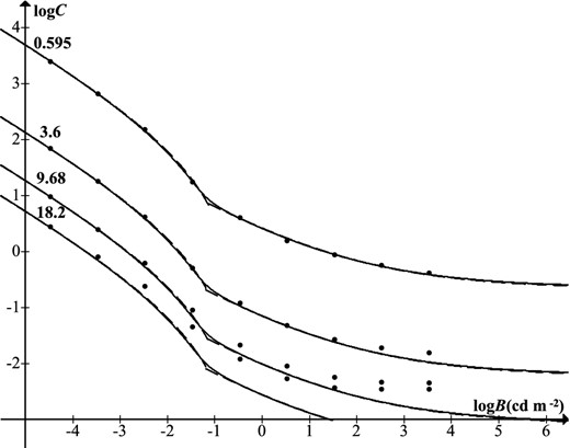
In either case, we can compare the resulting function C = R/A with the original data set. This is seen in the uppermost curve of Fig. 6 which shows that both model versions fit the data very well, and apart from the transition region around B = 7.08 × 10⁻² cd m−2 (15.5 mag arcsec−2) they are virtually indistinguishable. One expects the point-source model to maintain accuracy across the range of validity of Ricco's law, i.e. for target sizes up to the Ricco area. For daylight conditions this means a diameter of no more than about an arcminute, but in low light conditions the size increases. This is seen in the lower curves of Fig. 6, which show that at low light levels the point-source model remains highly accurate for target diameters up to about 10 arcmin.
Henceforth, only the Blackwell values (equations 26–28) will be used. It will be noted that the model (equations 32–34) does not have the correct asymptotic limit as B → 0, since the threshold should tend to a non-zero value. This defect is not important for naked-eye astronomical observation, because of the natural brightness of the sky, but is relevant in telescopic observation, and will be addressed later.
2.3 Full visibility model
To construct the complete model, it is necessary to find an analytic expression for C∞, the threshold for large targets. At daytime luminance levels C∞ is independent of B (reflecting Weber's law) and ‘large’ is only a few arcminutes, but at low levels it rises above 6°, the maximum target size in Blackwell (1946). Taylor (1960a) attempted to extend Blackwell's data in order to find C∞ (at detection probability 0.5) for all background luminance levels, though he used a lower colour temperature (2360 K), fixed viewing time (6 s) and a rather different methodology. His results were somewhat inconsistent with Blackwell's (Taylor 1960b), with thresholds higher by a factor of approximately 2.2 for B of the order of 1 cd m−2, and approximately equal for B of the order of 10−3 cd m−2 or less.
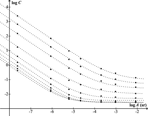
Contrast threshold versus target size (equation 41) for luminances at intervals of one log-unit, B = 3.426 × 10⁻⁵–3.426 × 10³ cd m−2 (top to bottom). Data from Blackwell (1946). Top four curves modelled by equations (23), (26), (35), (37) and (44); middle two by equations (25), (28), (39), (40), (42) and (43); bottom three by equations (24), (27), (36), (38) and (42).
3 ASTRONOMICAL VISIBILITY
3.1 Naked-eye
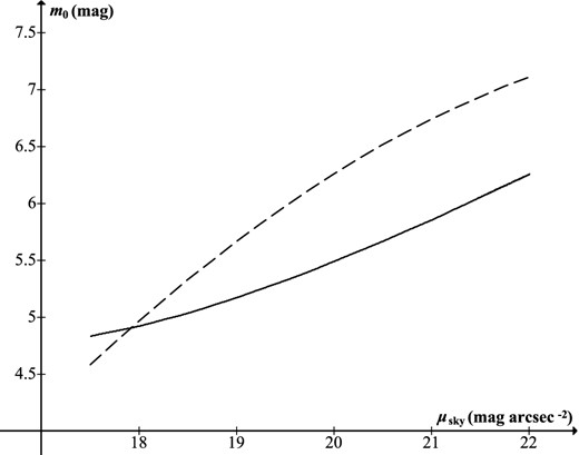
For a dark sky with B = 2 × 10⁻⁴ cd m−2 (21.83 mag arcsec−2), equation (53) gives a magnitude limit m0 = 6.93 − 2.5 logF. This would suggest that in actual observing situations F is typically somewhere between 2.4 and 1.4 (giving limits 5.98–6.57 mag), with 7 mag corresponding to F = 0.94. In view of the historical evidence discussed earlier, it would seem that for illustrative purposes a notional value F = 2 (limit 6.18 mag) could be taken as a typical overall field factor. Fig. 11 shows limiting magnitude as a function of sky surface brightness from equation (53) with F = 2. Also plotted is equation (20) converted to astronomical units (without field factor rescaling). Either curve can be moved up or down by a choice of overall field factor; what is significant is the incorrect curvature of Hecht's formula remarked earlier (reversed now because of the change to astronomical units).
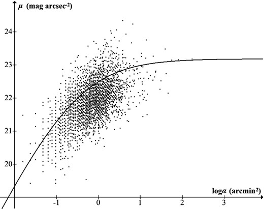
This can be applied to the visibility of M33. Weaver (1947) cited Lundmark's ability to see the galaxy without aid as an example of exceptional acuity, but at a Bortle Class 1 site it is an ‘obvious naked-eye object’, and it is only in the fifth out of nine classes (‘suburban sky’) that M33 is considered undetectable (Bortle 2001). Tables 2 and 4 of De Vaucouleurs (1959) give the galaxy's total magnitude as 5.8, suggesting easy visibility at a dark site, but the foregoing remarks imply that a fainter stellar limit would be required. The data give an equivalent circular radius of 25.3 arcmin, but this is to an isophote 25.3 mag arcsec−2, fainter than the eye can detect.
Fig. 12 plots surface brightness versus log-area, so any line μ = 2.5 logα + c is a line of constant magnitude c − 5 log60. Data points show the enclosed area and average surface brightness for successive isophotes of M33 (with an interpolated curve, dashed) as well as the threshold curve equation (58) (curve A, solid) for a background μsky = 21.83 mag arcsec−2 and F = 1.378, the latter parameter having been chosen so that the two curves are just touching, i.e. the target is at threshold. Raising F will shift the threshold curve downwards, so the target becomes invisible. The coordinates of the intersection point give the visible size and brightness of the galaxy: equivalent circular radius 18.7 arcmin, surface brightness 22.43 mag arcsec−2, magnitude 5.93. The Ricco asymptote is a line of constant magnitude 6.59 (the stellar limit required for the target to be visible) while the horizontal asymptote shows a large-target limit 24.59 mag arcsec−2.
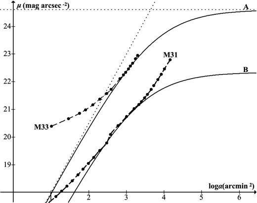
The same procedure can be repeated for different values of the surrounding sky background μsky (the zenith value would generally be darker). Visibility at F = 2 is found to require μsky = 22.63 mag arcsec−2, darker than the natural sky. For 21 ≤ μsky ≤ 22 mag arcsec−2, F ≈ 0.5482μsky − 10.585 (maximum error 0.02). As μsky increases within this range, the meeting point of the curves moves very little (slowly upwards), so that for all μsky the visible target has total magnitude 5.9 while the required stellar limit falls slowly from 6.67 to 6.57 mag. The visible radius and surface brightness hardly change as darkness increases within the stated range (18.5-18.75 arcmin, 22.41-22.44 mag arcsec−2); both differ substantially from the figures measured to the 25.3 mag arcsec−2 isophote, and instead refer to an (interpolated) isophotal limit 23.71-23.75 mag arcsec−2. Some caution is necessary since the target is neither uniform nor circular, and the edge is actually seen against the (invisible) remainder of the galaxy rather than the sky, but the general conclusion (given the low F values required) is that M33 cannot reasonably be considered an easy target for average observers, even under very dark skies. Since the condition of its being just visible is a sustained limiting stellar magnitude of approximately 6.6 (certainly achievable under dark skies by observers with above-average acuity), the required magnitude limit can be taken as a sufficient sky quality indicator. That figure, which can be thought of as the galaxy's ‘effective’ visual magnitude, is consistent with the visual estimate of approximately 7 mag made by Holetschek (1907) and accepted by Hubble (1926). As noted earlier, the galaxy was included by Heis (1872) in his naked-eye star atlas which had stellar limit 6.7 mag. Weaver (1947) gave the galaxy's visual magnitude as 6.8 mag.
A similar procedure can be applied to M31 using data from De Vaucouleurs (1958). It is found that with F = 2 the galaxy should become just visible at approximately μsky = 19.2 mag arcsec−2 (curve B on Fig. 12), with visible area approximately 2100 arcmin2 and effective visual magnitude 5.2. This must be treated with caution since the luminance is close to mesopic; however, the general prediction is that M31 should be an easy naked-eye target for average observers under moderately dark conditions, which accords with experience.
One should also consider the (B − V) colour indices of M31 and M33, given by De Vaucouleurs as 0.91 and 0.55. Cinzano et al. (2001) took the typical colour index of naked-eye stars as 0.7, and if this is considered the standard by which visual threshold is assessed then (from equation 18) the effective magnitude of M31 should be lowered by 0.06 while that of M33 should be raised by 0.04. If colour index 0 is the standard then the effective magnitudes of M31 and M33 are instead lowered by 0.25 and 0.15.
3.2 Point-source telescopic visibility
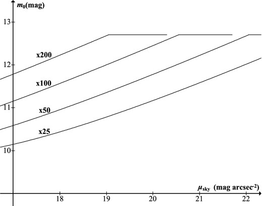
Magnitude limit m0 as a function of sky brightness μsky, calculated from equation (68) (with FtFMFTF = 3.77, p = 7 mm) for a telescope with clear aperture 100 mm at various magnifications. The cut-off mcut = 12.7 mag is due to the background in the eyepiece becoming effectively zero.
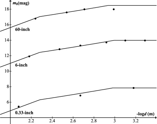
Magnitude limit m0 as a function of exit pupil d for three telescopes (labelled by aperture). Data from Bowen (1947), modelled with equations (68) and (71). The anomalous data point for the 60-inch at highest magnification, attributable to the stellar disc being no longer point like, is modelled in Section 3.3.
Magnitude penalty pen = m22 − m0 and surface-brightness supplement sup = μ∞ − m0 with respect to ideal conditions (μsky = 22 mag arcsec−2), with approximate sky-quality banding.
| Pristine | Black | Grey | Grey | Bright | ||||||||
|---|---|---|---|---|---|---|---|---|---|---|---|---|
| μsky | 22.00 | 21.75 | 21.50 | 21.25 | 21.00 | 20.75 | 20.50 | 20.25 | 20.00 | 19.75 | 19.50 | 19.25 |
| pen | 0.00 | 0.10 | 0.20 | 0.30 | 0.40 | 0.49 | 0.59 | 0.68 | 0.77 | 0.85 | 0.93 | 1.01 |
| sup | 18.06 | 17.98 | 17.90 | 17.82 | 17.74 | 17.66 | 17.58 | 17.49 | 17.40 | 17.32 | 17.22 | 17.13 |
The minimum possible value for Ft would have been 1.04 (1 per cent reflectance at four coated glass-air surfaces for a refractor with no light scattering). From the B/Ft value for the telescope with lowest Ft (0.33 inch), this produces a lowest bound B = 3.12 × 10⁻⁴ cd m−2 (21.35 mag arcsec−2). Realistically estimating 90 ± 5 per cent transmittance for the 0.33-inch telescope, the previously calculated ratios give transmittances 81 ± 4.5 per cent for the 6-inch and 60 ± 3.3 per cent for the 60-inch telescopes, the latter implying a reflectance of approximately 85 per cent at each of the three aluminized mirrors, a plausible figure not far below the maximum value of 89 per cent. The figure for the 6-inch refractor could suggest it was in need of cleaning, or did not have antireflection coating as Bowen stated (having the equivalent of 95 per cent transmittance at each air-glass surface), or perhaps the clear aperture was actually slightly less than the assumed value.
The figures imply a sky brightness B = 3.34 ± 0.19 × 10⁻⁴ cd m−2 (μsky = 21.27 ± 0.06 mag arcsec−2). Assuming |$F_{\rm{M}}F_{\rm{T}} = \sqrt{2}$| as usual, F is then 2.74 ± 0.15, somewhat higher than the ‘typical’ value 2 but consistent with Bowen's age, and giving his naked-eye limit (from equation 53) as 5.62 ± 0.04 mag. If he had recorded his naked-eye limit then the transmittances and sky brightness could have been determined from that.
Garstang (2000) analysed Bowen's data using a modified form of the Hecht equation, employing the enumerated field factor treatment of Schaefer (1990). He made estimates of various parameters in his model, and arrived at a predicted sky brightness B = 1.05 × 10⁻³ cd m−2 (μsky = 20.03 mag arcsec−2), substantially brighter than the new estimate. Garstang made an airmass correction based on a guess of the zenith angle of observed stars, to arrive at a zenith brightness B = 8.59 × 10⁻⁴ cd m−2 (μsky = 20.24 mag arcsec−2). When the same correction is made to the new figure, one obtains B = 2.45 × 10⁻⁴ cd m−2 (μsky = 21.61 mag arcsec−2).
Garstang (2004) calculated the sky brightness at Mount Wilson throughout the twentieth century using his light-pollution model, for which a crucial parameter is the average light emission per head of population. Garstang estimated this parameter, guided partly by his analysis of Bowen's data, producing results somewhat darker than his previous work (20.82 mag arcsec−2 for 1950), but still considerably brighter than the new estimate. The present finding suggests that light emissions from Los Angeles in the first half of the twentieth century were lower than Garstang assumed, and that the growth of light pollution in the second half was far more rapid than he calculated.
3.3 The telescopic threshold curve
Bowen (1947) obtained a limit 18 mag for stars seen with the 60-inch telescope at M = 1500, rather than the predicted point-source limit 18.7 mag. From Fig. 14, it can be seen that this was against an effectively zero background. With the parameters derived earlier, one finds αTR0 = 7.012 × 10⁻³ arcmin2, and equation (88) can be solved for α (with m0 − mlim = 0.7). If this is interpreted as the area of the Gaussian stellar disc (with due caution regarding the target's non-uniformity), then it gives the diameter as 3.0 arcsec, and from Section 1.6.2 the FWHM seeing is estimated as 3.0/2.8 = 1.1 arcsec, entirely consistent with Bowen's remark that it was ‘about average’.
The model can be applied to the observations of William Herschel, who compiled three catalogues of ‘nebulae’ (mostly galaxies) discovered between 1783 and 1802 with a telescope which had an 18.7-inch (475.0 mm) diameter speculum mirror and ‘sweeping power’ M = 157 (Herschel 1912, vol. 1, p. 260). From 1786 he used the telescope in ‘front-view’ mode, without a secondary mirror (Herschel 1912, vol. 1, p. xlii) so that the entrance pupil was equal to the full aperture (assuming his head did not intrude) and the exit pupil diameter was d = 3.03 mm. In 1801, by looking at the star Vega through artificial pupils of various sizes, he measured his eye pupil as 0.2 inch (5.08 mm; Herschel 1912, vol. 2, p. 585). He visually measured the reflectance of his mirror as 67 per cent and determined the overall transmittance (in front-view mode with a single-element eyepiece) as 63.8 per cent (Herschel 1912, vol. 2, p. 40), very close to the modern theoretical figure 0.68 × 0.962 = 62.7 per cent, which gives Ft = 1.6 for his telescope at best performance. The sky brightness would have varied during the observing period due to solar activity, but sunspot data are sparse (Zolotova & Ponyavin 2011). The figure B = 2 × 10⁻⁴ cd m−2 (21.83 mag arcsec−2) will be taken as an approximation. From equation (70), this gives d0 = 1.45 mm with M = 328.
If it is assumed as before that |$\phi = \sqrt{2}F$|, where F is the naked-eye field factor, then ϕ can be determined from Herschel's naked-eye limiting magnitude. An indication of this is that he found Uranus (5.9 mag at its faintest) a near-threshold object (Herschel 1912, vol. 1, p. 106), but more precise is his remark on double star H I 69 (CCDM J07057+5245AB) which he discovered in 1782: ‘in a very clear evening it may just be seen with the naked eye’ (Herschel 1912, vol. 1, p. 333). This system, which Herschel would have been able to view almost exactly at the zenith, has integrated magnitude 6.12 and colour index 0.1. The average colour index of objects in the NGC is 0.85 (Steinicke 2014a), for which the corresponding limit would be 5.92 (from equation 18); but Herschel may have been able to see objects slightly fainter than H I 69. As an approximation, his limit will be taken as 6.0 mag (with respect to assumed colour index 0.85).
It will be noted that nearly 20 years elapsed between Herschel's naked-eye star observation (aged 44) and his measurement of his eye pupil (aged 63), and it is entirely possible that both figures would have changed over that period. One could also question the assumption |$\phi = \sqrt{2}F$| since the factors are not for equivalent search procedures: Herschel's telescopic search was for objects not previously known, whereas his naked-eye observation was of a star whose position he knew in advance. Moreover, the front-view mode would have introduced aberration because the mirror was viewed at an angle to the optical axis, and more generally his telescope cannot have been optically perfect. Nevertheless, the stated figures will be adopted for calculation purposes.
From equation (53) with the assumed sky brightness, we find F = 2.36. From equation (87) this implies that Herschel's limit for stars seen with the telescope at sweeping power M = 157 would have been 15.66 mag in front-view mode and 0.24 mag poorer in Newtonian mode (assuming 67 per cent reflectance for the secondary, and without correction for the central obstruction whose size is not recorded). This is consistent with the magnitude limit of his catalogue: out of roughly 2500 nebulae Herschel discovered, only 7 are 15.0 mag or fainter (Steinicke 2014b), down to a minimum of 15.5 mag for NGC 2843 and NGC 4879, the latter being a misidentified star. For verifying objects, Herschel sometimes used M = 240 (Herschel 1912, vol. 1, p. 268), with a predicted front-view limit 16.08 mag. The cut-off for M ≥ 328 would have been 16.39 mag.
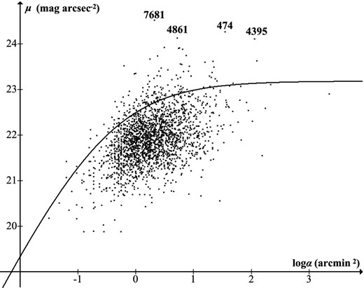
Objects found by William Herschel, plotted by surface brightness μ versus area α. 91.7 per cent lie below his predicted threshold curve (equation 89); some extreme outliers (labelled by NGC number) are discussed in the text.
Some extreme outliers are marked on Fig. 15 by their NGC numbers; in all cases, Herschel did not see the complete object. Herschel estimated NGC 4395 (H V 29) as ‘10 arcmin long, 8 or 9 arcmin broad’ (Herschel 1912, vol. 1, p. 359), which is only about 60 per cent of its actual area (three of its H ii regions became designated as separate nebulae in the NGC). He saw NGC 4861 (H IV 30) as ‘two stars, distance 3 arcmin, connected with a very faint narrow nebulosity’ (Herschel 1912, vol. 1, p. 356), but the galaxy is approximately 40 per cent longer. He described NGC 7681 (H II 242) as ‘small’ (Herschel 1912, vol. 1, p. 275) and NGC 474 (H III 251) as ‘very small’ (Herschel 1912, vol. 1, p. 284).
Fig. 16 shows NGC objects which Herschel failed to discover (3431 objects with declination higher than −33°, unknown to Herschel, for which magnitude and area data are available in Steinicke (2014a,b), using Epoch 2000.0 coordinates and without atmospheric or photometric correction). Herschel did not sweep the entire sky above his horizon (Steinicke 2010, p. 34), and this can account for some of the omissions. Others could have been missed because of low declination, crowded search fields, proximity to glare sources (bright stars), limited search time or human error. In general, however, it can be seen that the missed objects are smaller and nearer threshold than the discovered ones. This can be quantified using ‘visibility level’, defined as the ratio of an object's contrast to the threshold level (Adrian 1989), for which the corresponding astronomical quantity is the object's distance (L) below the curve. For the objects in Fig. 15 mean L is 0.69, and mean logα is 0.28, whereas for the missed objects mean L is 0.35, mean logα is −0.21. Missed objects with α and L larger than the mean values for discovered ones, and which therefore should have been easy targets for Herschel, amount to only 3.6 per cent of those he did not see, illustrating the thoroughness of his search.
NGC objects missed by William Herschel. These are generally smaller, and nearer to his threshold, than those in Fig. 15. 90.6 per cent of missed objects below the curve are smaller than the average size of objects he detected.
3.4 Further applications
There has been interest among visual astronomers in the concept of ‘optimum magnification’ (Lewis 1913; Clark 1990; Garstang 1999). The contrast of an extended object seen in a telescope is independent of magnification, but the threshold is dependent on image size and background, both of which change with magnification. Hence, an object may be invisible at low or high power but visible in some intermediate range. This is represented in Fig. 17 which shows threshold curves for a 100 mm telescope at magnifications 20, 75 and 200 (with parameters chosen for convenience of illustration), and a single data point representing a hypothetical non-stellar object. Raising power shifts the Ricco asymptote to the left (increasing the point-source limit) but lowers the horizontal asymptote (decreasing the surface-brightness limit). The object is predicted to be visible at magnification 75 but not at the lower and higher powers. The model could be used to obtain optimum magnifications for actual objects, but such predictions are of limited value, both because of the lack of appropriate data at the correct isophotal limit, and (most importantly) because targets are in general not uniform. It is however interesting to note the finding of Leibowitz (1952) that at low light levels visual acuity is greatest for a pupil size of approximately 3 mm. This corresponds to the exit pupil chosen by William Herschel for his nebula sweeps, which he presumably arrived at using trial and error. The same optimum exit pupil was found independently by Langley (2004).
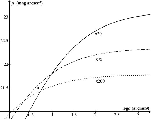
Threshold curves for a 100 mm telescope at various magnifications (with μsky = 21.4 mag arcsec−2, p = 6 mm, Ft = 1.04, ϕ = 3.55). The data point is for an object predicted to be visible at × 75 but invisible at the lower and higher powers.
It is interesting to make general comparative predictions of instrument performance. Fig. 18 shows threshold curves for a single user (p = 7 mm, F = 2) at two sites, one light polluted (μsky = 20 mag arcsec−2, naked-eye limit 5.5 mag), the other dark (μsky = 21.5 mag arcsec−2, 6.0 mag). The instruments are 10 × 50 binoculars and a 6-inch refractor (D = 150 mm) at the dark site, and a 16-inch reflector with 25 per cent central obstruction (D = 393 mm) at the light polluted one, with assumed transmittances 85, 95 and 75 per cent, respectively. Both telescopes have exit pupil 3 mm. Data are also plotted for the 16 Messier galaxies in the Virgo Cluster (Steinicke 2014a), subject to the usual caveats regarding isophotal limit and non-uniformity, but providing a reasonably homogeneous sample for illustrative purposes. It can be seen that for any target larger than 1 arcmin2 the 16 inch is outperformed by the smaller telescope at the darker site: light pollution renders it ineffective for viewing galaxies. Binoculars outperform the 6 inch for very large, low surface-brightness objects; however, the 6 inch will show numerous smaller targets. Since the effect of varying the field factor F is to move all the curves up or down equally, this qualitative result will remain the same for individuals whose naked-eye limit is higher or lower than the chosen figure.
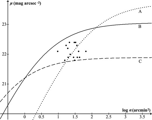
Threshold curves for various viewing situations. Curve A is for 10 × 50 binoculars at a dark site (μsky = 21.5 mag arcsec−2), curve B is a 6-inch refractor with exit pupil 3 mm at the same site, and curve C is a 16-inch reflector with the same exit pupil at a light-polluted site (μsky = 20 mag arcsec−2). Data points are for Messier galaxies in the Virgo Cluster.
4 CONCLUSIONS
A new way has been presented for modelling achromatic threshold visibility data such as that of Blackwell (1946) or Knoll et al. (1946), and has been shown to represent the laboratory data more accurately than previous models. For applications at low light levels, a photometric correction is needed; this has been calculated for scotopic vision, applicable to astronomical observations within approximately 1 mag of threshold at sites without excessive light pollution. The new point-source model matches the data of Bowen (1947) more accurately than previous attempts by Schaefer (1990) and Garstang (2000). The model for extended targets offers new insights into the visibility of ‘deep sky objects’ such as galaxies, and has been shown to be consistent with the observations of William Herschel.
The basic relation of the model, shown in Figs 5 and 8, was purely empirical, but one might question whether it has a physiological basis. Equation (23) implies |$C \approx (r_{1}^2/A)B^{-1/2}$|, the de Vries Rose law (Rose 1948), so the relation models the departure of the visual system from ideal quantum detection, which is presumed to arise at the stage of post-retinal processing. Because the visual system is quite different from a detector limited only by quantum efficiency, the results presented here are not expected to be applicable to CCD imaging. However, since a similar threshold curve is obtained for targets identified visually from photographic plates (Hubble 1932), one would expect applicability there. Any line of constant magnitude brighter than the Ricco asymptote will intersect the threshold curve, demarcating zones that are visible or otherwise. Hence, the completeness of any magnitude-limited sample is dictated by the shape of the curve together with the luminosity function for the targets in question. This should apply for example to the catalogue of Shapley & Ames (1932), for which an empirical completeness function was found by Sandage, Tammann & Yahil (1979).
The photopic model of Section 2 would be applicable to daylight phenomena such as sunspots, though visibility of objects against the blue sky would require proper incorporation of chromaticity. This would also be the case for mesopic applications, e.g. observation at heavily light-polluted sites where colour can be perceived. Successful modelling of situations such as these would require new experimental data sets, other than the achromatic ones used here. At light-polluted sites where scotopic vision is possible (i.e. darker than about 19 mag arcsec−2), the sky spectrum will have anthropogenic contributions for which a photometric correction is necessary, as shown in Section 1.3.
Photometers are available which measure both photopic and scotopic luminance. This would be useful in light-pollution studies since S/P ratio varies with type of lighting: a moonlit country sky and a moon-less suburban one polluted by fluorescent lighting could both give the same reading on a Sky Quality Meter (e.g. 20 magSQ arcsec−2, or ‘SQ 20’), but the country sky would be brighter to scotopic vision since the S/P ratio of fluorescent lighting is generally lower than that of moonlight. If the meter were fitted with a removable scotopic filter and suitably calibrated then S/P ratios could be found and quoted in addition to photopic luminance.
The International Dark-Sky Association (IDA 2013) currently recognizes three classes of dark sky: bronze (SQ 20.00–20.99), silver (SQ 21.00–21.74) and gold (SQ ≥ 21.75). A reading greater than 22 is ‘unlikely to be recorded’ (Unihedron 2014b). The suggested limiting magnitudes (based on the Bortle Scale) are bronze: 5.0–5.9, silver: 6.0–6.7, gold: ≥ 6.8. It is questionable whether 20 mag arcsec−2 can be considered dark, given the results shown in Fig. 18. Also, it has been argued here that a definition of naked-eye limiting magnitude based on momentary glimpses is overly susceptible to scintillation, which is a local and variable effect. Consequently, it has been suggested that currently recommended magnitude limits may be excessive, compared with limits that would be obtained for targets visible for an extended period. It has also been shown that the recommendations of the Bortle Scale with regard to the visibility of M33 are contradicted by the present model. Since the scale appears to be based on subjective judgment rather than rigorous data, its reliability appears questionable.
A practical definition of a dark sky would be one in which the Milky Way is capable of being seen. The non-uniformity of the Milky Way makes this problematic to model, and even if a particular region were chosen as standard, there remains the problem that existing luminance measurements are based on a surface-brightness limit fainter than that of the eye, and are usually filtered to remove bright stars, whereas unresolved stars just beyond the visual limit may contribute a significant proportion of the light detectable by eye. An equivalent limiting magnitude could be found empirically: observers would view the sky through a variable filter, adjusting it until a chosen portion of the Milky Way was considered just visible, and they would also note the faintest stars visible at this setting.
Bigourdan (1917) noted that the summer Milky Way became visible from Paris Observatory when the Sun reached 13° below horizon. The corresponding sky brightness is dependent on local conditions but would have been approximately 20.2–20.3 mag arcsec−2 (Patat et al. 2006). Bigourdan further noted that with the Sun 15° below horizon he was able to see faint NGC objects, while an angle of 16° was sufficient for the faintest to become visible. That would indicate approximate values of 21.3 and 21.5 mag arcsec−2. That suggests a three-tier dark-sky classification with proportionally diminishing SQ bands 20.25–21.24 (‘grey’), 21.25–21.74 (‘black’) and 21.75-22.00 (‘pristine’). Recalling, from Section 1.3, the CIE (2010) suggested limit for scotopic vision, one could add a ‘bright’ band SQ 18.25–20.24, and a ‘white’ band SQ <18.25, in which scotopic vision would not be achievable for naked-eye sky observation.
This work was begun while the author was Visiting Fellow at Durham Institute of Advanced Study. The author warmly thanks Martin Banks (Berkeley) and Gordon Love (Durham) for invaluable conversations during that initial phase of the project.
