

Abstract
We study correlations of non-affine displacements during simple shear deformation of Cu–Zr bulk metallic glasses in molecular dynamics calculations. In the elastic regime, our calculations show exponential correlation with a decay length that we interpret as the size of a shear transformation zone in the elastic regime. This correlation length becomes system-size dependent beyond the yield transition as our calculation develops a shear band, indicative of a diverging length scale. We discuss these observations in the context of a recent proposition of yield as a first-order phase transition.
Export citation and abstract BibTeX RIS

Original content from this work may be used under the terms of the Creative Commons Attribution 3.0 licence. Any further distribution of this work must maintain attribution to the author(s) and the title of the work, journal citation and DOI.
1. Introduction
Bulk metallic glasses (BMGs), multi-component metals that are kinetically arrested into an amorphous structure, have been suggested for wide range of applications, including as structural materials [1, 2]. For practical applications a big problem is their tendency to form shear bands [3], planar regions in that localize most of the plastic deformation at relatively low strain [4, 5]. These shear bands are the primary mechanism by which metallic glasses fail in tensile [6] or cyclic (fatigue) loading [7, 8] or during indentation [9]. Numerous ideas to address this problem have been suggested, such as deliberately introducing heterogeneities, such as pores [10], nanocrystals [11] or internal interfaces [12].
The deformation of BMGs is described by the theory of shear transformations or shear transformation zones (STZs) [13–15], localized rearrangements of small regions of atoms. The size of these zones has been estimated to range from a few [16] to many tens of atoms [17, 18]. Knowledge of the size of the zones could help to fundamentally understand this class of materials on an atomic level and be used in mesoscale simulations that incorporate STZs [19–21]. The size of STZs has been linked to the Poisson ratio [22] as well as the brittle or ductile character of fracture of BMGs [23–25].
Spatial correlation functions of non-affine deformation have recently been employed to quantify the geometry of STZs. Murali et al [26] looked at the spatial autocorrelation in the non-affine deformation field of deformed BMGs in molecular dynamics (MD) simulations. They found an exponential decay of the autocorrelation from which they extracted a correlation length  which they interpreted as the size of an STZ. These findings have been confirmed by similar calculations on Lennard-Jones-Glasses [27]. In a similar spirit, Chikkadi et al [28, 29] have discussed the autocorrelation of non-affine deformation in experiments of sheared colloidal glasses. In addition to the global non-affine displacement field, they characterized the local non-affine deformation through the
  measure of Falk and Langer [15]. Their data shows long-range correlations as manifested in a power-law behavior of the autocorrelation function in both global and local measures for non-affinity. In contrast to Murali et al's data [26], this suggests a scale-free character of the deformation. Calculations of hard-sphere mixtures carried out for the interpretation of these experiments did again yield an exponential decay of the correlation function [29, 30]. Varnik et al [31] argued that this is because of limitation in system size; larger calculation, albeit carried for a 2D soft disk model rather than in 3D, indeed showed power-law correlations. In a large study comparing different simulation models and experiments, Cubuk et al [32] appear to find again only exponential correlation in
  Note that correlation of the vorticity (strain) field during deformation of a 2D Lennard-Jones solid showed similar power-law correlations [33, 34], and we have recently found power-law correlation in the displacement-difference field [35]. The question of power-law versus exponential correlation clearly hinges on the details of the quantity whose correlations are studied.
We here revisit the question of exponential versus power-law correlations in  provide new data on how they evolve through the yield transition and show that the question of exponential versus power-law correlation depends on how
  is calculated. Our MD calculations of the deformation of BMGs show the emergence of correlations in the non-affine part of the deformation field of calculations larger than those previously reported. This allows us to extract the correlation function up to distance ≈75 times the nearest neighbor distance for the largest systems studied here, similar to previous 2D calculations that showed power-law correlation [31]. While we do find exponential and not power-law correlations, the length-scale
  associated with the exponential becomes a function of system size after shear-band nucleation, indicating a divergent length at the nucleation of the band, but only if the 'strain window' used to calculate
  is chosen large enough.
2. Methods
2.1. MD simulations
We conducted all simulations using MD and the second generation of the interatomic Cu–Zr potential by Mendelev et al [36]. Amorphous sample systems were first obtained by melting and equilibrating systems of Cu50Zr50 (or other stoichiometries, see below) at 2500 K for 100 ps, followed by a linear quench to 750 K at a rate of 6 K ps−1. This temperature is slightly above the glass transition temperature  as obtained from the jump in heat capacity when cooling the system through Tg at the same rate. We then aged the system for 1 ns before quenching it to 0 K at a rate of 6 K ps−1. We used a Berendsen barostat [37] with a relaxation time constant of 10 ps to keep the hydrostatic pressure in the simulation cell at zero and Langevin thermostat [38] with a relaxation time constant of 1 ps to control temperature during quench and equilibration.
To prepare simulations carried out at different temperatures, the amorphous systems were then equilibrated at zero pressure for 200 ps at different temperatures between 0 and 300 K. The cell was subsequently deformed using simple shear deformation at constant volume at an applied shear rate of  up to a maximum of 35% strain. To control temperature, we again used a Langevin thermostat but only thermalize the Cartesian direction normal to the plane of shear to eliminate any drag with respect to the reference velocity field intrinsic to the Langevin thermostat. The bulk of our simulations comprises a cubic cell with an edge length of
  and 500 000 atoms. The potential influence of finite-size effects was studied using two additional system sizes: A cubic system with twice the edge length and eight times the number of atoms and another cubic system with half the edge length and 1/8 the number of atoms. We ran all sets of parameters for five systems obtained from independent quenches and averaged the results of the analyses, to reduce the impact of random fluctuations. If not mentioned otherwise, results are reported for the
  systems and as averages over these five realizations.
2.2. Local strain measure and correlation
To quantify heterogeneous flow of the system, we need measures that identify local deformation events. Falk and Langer [15] introduced a method to determine the local deformation of an atomic system within spheres of radius rcut. The idea is to map for each atom i its atomic neighborhood at time t–∆t to the neighborhood at time t using an affine deformation with deformation gradient  and then find
  that minimizes the residual error. The final residual error

is a measure for the non-affine component of local deformation. Here  is the Heaviside step function. STZs and shear bands can be identified by looking for regions with high values of
  Note that for our calculations carried out at constant applied shear rate
  we specify the reference frame by its distance in applied strain
  the strain window, rather than
To quantify the geometry of these deformation events, we use spatial auto-correlation maps. The auto-correlation map of some field  is defined as

where the last identity is the expression obtained for  point particles for which
  where
where  is the value of quantity
  on atom
  Note that for any quantity
  this autocorrelation map obeys the following sum rules

where the average 
The radial average of this auto-correlation map gives a function ,$](https://content.cld.iop.org/journals/2515-7639/2/4/045006/revision2/jpmaterab36edieqn27.gif) depending only on the distance and not the direction between the two atoms. The auto-correlation function of unity is the radial distribution (or pair correlation) function
depending only on the distance and not the direction between the two atoms. The auto-correlation function of unity is the radial distribution (or pair correlation) function

By virtue of equation (3) it is normalized such that  as
as  We are specifically interested in the correlations of

Note that equation (5) is normalized such that, because of equation (3),  and
and  We compute
 $](https://content.cld.iop.org/journals/2515-7639/2/4/045006/revision2/jpmaterab36edieqn33.gif) at short distances by direct evaluation of equation (2) and at long distances using a fast Fourier transform to speed up the convolution in equation (2), allowing us to efficiently compute the correlation function up to half the size of our systems. Details of this algorithm are given in the appendix.
at short distances by direct evaluation of equation (2) and at long distances using a fast Fourier transform to speed up the convolution in equation (2), allowing us to efficiently compute the correlation function up to half the size of our systems. Details of this algorithm are given in the appendix.
3. Results
Figure 1(a) shows a snapshot of the quenched system before shear. The radial distribution function  (figure 2(a)) is indicative of a disordered structure with broad nearest and second-nearest neighbor peaks and non-zero probability for finding a neighbor between them. The first neighbor peak is located at
  and indicated by a vertical dashed line and we use rNN to normalize all distances reported below. The value of the non-affine displacement
  depends on the cutoff distance
  for identifying neighbors of an atom and on the distance
  between current and reference configuration in the time domain. In the following, we will show results obtained for
  being an integer multiple of the nearest-neighbor distance
  as given by the position of the first peak in
  These distances are indicated by the vertical dashed lines in figure 2(a).

Figure 1. Snapshots of the system at (a) 0%, (b) 25% and (c) 50% applied simple shear strain. Arrows indicate the shearing direction.
Download figure:
Standard image High-resolution image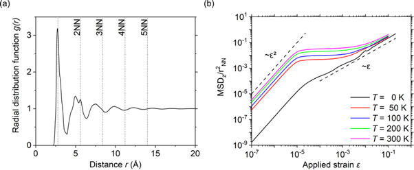
Figure 2. (a) Radial distribution function of the CuZr BMG at 0 K. Vertical lines represent multiples of the nearest neighbor distance rNN = 2. 8 Å used as dcut for the calculation of D2min. (b) Mean squared displacements in the z direction (perpendicular to the simple shear plane). Dashed lines show ∼ε2 (diffusive) and ∼ε (ballistic) scaling.
Download figure:
Standard image High-resolution imageAfter equilibrating, we deformed our metallic glass under simple shear. Figures 1(b) and (c) show exemplary snapshots of these calculations. As an important dynamical quantity, we analyzed the mean square displacement (MSD) as a function of applied strain  where we only considered the component of the displacement in the z-direction, perpendicular to the plane where shear is applied (figure 2(b)). This is necessary in order not to contaminate the displacement by the applied shear; we could have subtracted the streaming velocity alternatively. Note that at constant strain rate
  the applied strain
  is the same as the usual parameter time t. The MSD shows the typical behavior for a glass [39]: initially,
  showing the ballistic motion of each atom within its local environment. The MSD then saturates at a value ≈0.01 rNN, corresponding to a distance of around 0.1 rNN2 much smaller than the nearest neighbor distance (see figure 2(a)) but around the Lindemann criterion for melting [40]. Atoms do not diffusive in this regime but are trapped within their local cages. Finally, at large
  the system entered a diffusive regime where
  This diffusive regime is accompanied by a breaking out of the individual cage, because the mean distance traveled by the atoms now exceeds the nearest neighbor distance. Without mechanical agitation, this breaking out of the cage happens after what is known as the
  -relaxation time. Under mechanical agitation, it happens at the cage-breaking strain
  here between
  and 1% (see also [41, 42]).
The shear stress  in the plane of shear (figure 3(a)) initially rose linearly with the strain
  applied in the xy-plane. At around
  the system yielded and the stress
  dropped from a peak value to a plateau region where
  remained constant up to an applied strain of
  the maximum strain applied in our calculations. Our five calculations at 0, 50, 100, 200 and 300 K show that the system softened as temperature increased; from a yield stress of around 1.7 GPa in the athermal limit to 0.8 GPa at 300 K.

Figure 3. (a) Stress strain curves for CuZr at 0, 50, 100, 200 and 300 K. The region shaded in gray indicates the strains over which the systems show a sharp increase in ℓlong (see figure 8(a)). Black solid dots indicate the positions where the snapshots shown in (b)–(d) were taken. All calculations use rcut = 3 rNN and Δε = 1%. The color code corresponds to D2min with high values in red and low values in blue. At low strains (b) we find individual STZs. Higher strains (c) and (d) develop a clear shear band. (e) and (f) show the same state as (d), but D2min is computed at strain windows Δε = 0.1% and 0.01%, respectively. While individual events are still visible, there are not enough of them in the strain window to coalesce into a full band like in (d).
Download figure:
Standard image High-resolution imageFigures 3(b)–(d) show a map of  during deformation, here computed for a cutoff
  and a strain window of
  about the cage-breaking strain
  before the frame shown in the figure. At small strain
  where
where  is linear, we find localized events (figure 3(b)). After yield, these localized events coalesce to shear-bands, first vertical (figure 3(c), see also [27, 43–45]) but later horizontal (figure 3(d)), developing a clear anisotropic structure. Note that such vertical shear-bands occurred only in some of our calculations. At small strain, both shear-band directions are equivalent and the nucleation direction is random. Symmetry breaking at larger strain forces the shear band back into the direction of shear. We note that the shear-bands are only visible for strain windows
  Figures 3(e) and (f) show maps of
  for
for  and
and  respectively. Observed at these small strain windows, the shear band dissolves into individual disconnected localized events.
To statistically quantify this (random) structure we computed the  auto-correlation maps,
  Figures 4(a) and (b) show a slice
  Before yield (figure 4(a)),
  shows a rotationally symmetric structure with a visible ring at the nearest-neighbor distance
  After yield (figure 4(b)),
  develops an anisotropic structure with a band of correlation parallel to the x-axis. Figure 4(c) shows radial averages
  of the data of figures 4(a) and (b). There are oscillations at small distances that turn into an exponential decay at around 10 Å. Oscillations at small distances are due to the structure of the amorphous solid. We therefore normalize the autocorrelation function and define

to remove variations in  due to variations in local atomic density. The normalized correlations are also shown in figure 4(c). The oscillations are eliminated in
  for r > 5 Å. Note that beyond yield, the radial symmetry of
  is lost (see figure 4(b)). Figure 4(d) shows
  parallel and perpendicular to the shear band. The positions where the data is taken from is marked with the black and red line in figure 4(b). This shows that the correlation is practically constant in the shear band direction, while it decays perpendicular to it.
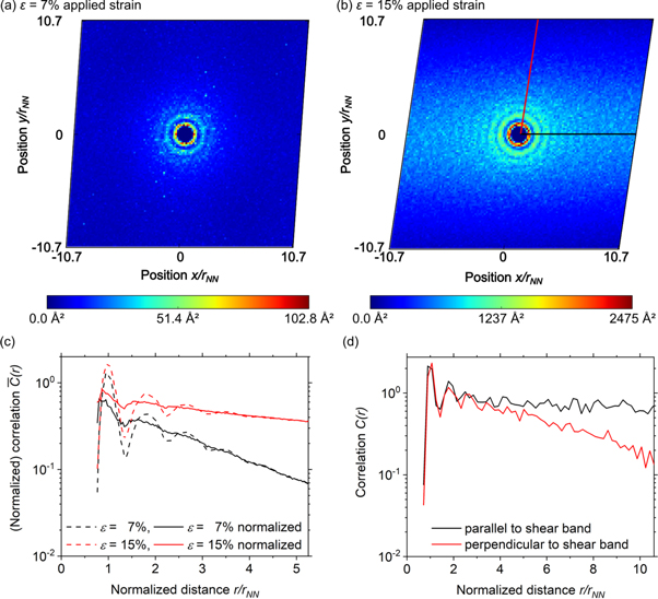
Figure 4. Slice through the normalized real space correlation in xy-plane at (a) 7% applied strain and (b) 15% applied strain. (c) Correlation function C(r) for the two cases shown in panels (a) and (b), both normalized (solid) and not normalized with pair correlation function g2(r) (dashed). (d) shows the correlation function from (b) parallel and perpendicular to the shear band (position indicated by the black and red line). All results are for a strain window Δε = 1%.
Download figure:
Standard image High-resolution imageThe radially averaged function  decays exponentially, as visible by a constant slope in the log-linear plots of figures 4(c), 5(a) and later. We find that there are two regions of exponential decay with different correlation lengths, clearly visible in figure 5(b). We characterize the exponential decay

by fitting the correlation length  in equation (7) over a select section of the correlation function. At short distance
  the characteristic length
  appears to be affected by the choice of
  within which the non-affine part of the local deformation field is computed, as presented in more detail below. The initial decay crosses over to a second exponential at distances
  with a characteristic length
  that does not depend on the specific choice of
  and reference frame and is a characteristic of the material under investigation.
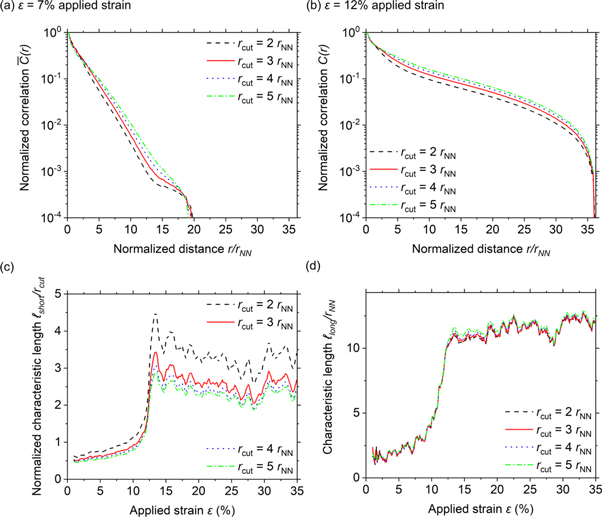
Figure 5. D2min auto-correlation functions at (a) 7% and (b) 12% strain, using different cutoff values rcut. (c) Characteristic length ℓshort derived from the correlations for the different cutoffs, normalized with the cutoff rcut for each line. (d) Bare unnormalized characteristic length ℓlong. All results are obtained for a strain window Δε = 1%.
Download figure:
Standard image High-resolution imageWe first focus on the behavior at short scales. The computation of  involves the cutoff radius rcut as a parameter. rcut determines the local atomic neighborhood within which
  is calculated. To test whether the length scales
  and
and  depend on this length, we parametrically vary rcut between rcut = 2 rNN = 5.6 Å and rcut = 5 rNN = 14 Å. The resulting correlation functions at 7% and 12% applied strain are shown in figures 5(a) and (b), respectively. The radius rcut varies by a factor of 2.5 while the individual correlation functions move systematically upwards. As a consequence, the extracted value
  depends systematically on rcut. Indeed, we can collapse all
  values on a single curve when normalizing by
 (figure 5(c)). The behavior of
  is different. Its value (figure 5(d)) is independent of
  used in the computation of
  and the data does not collapse when normalized accordingly. The evolution of
  and
and  with applied strain
  clearly show the point where the samples yield (see also figure 3(a)). At around 12.5% strain,
  increases dramatically. During further deformation it fluctuates around a value consistently higher by a factor of 4 than before yield.
The computation of  furthermore depends on how the reference frame for the computation of
  is chosen. Here, we report results obtained for reference frames at constant distance in applied strain,
  All results reported above were obtained for
  Figure 6 demonstrates how the correlation function and
  vary as a function of this parameter. Before yield, the correlation function does not depend on
  and drops exponentially over two decades as a function of distance. Figure 6(a) shows this behavior for
 and
and  which is above, at and below the cage-breaking strain
  (figure 2(b)). The behavior changes at yield (figure 6(b)), where the initial exponential drop starts to depend on
  Figure 6(c) shows the influence on the extracted value of
 decreases with decreasing
  and saturates at
  in the flow region for the lowest
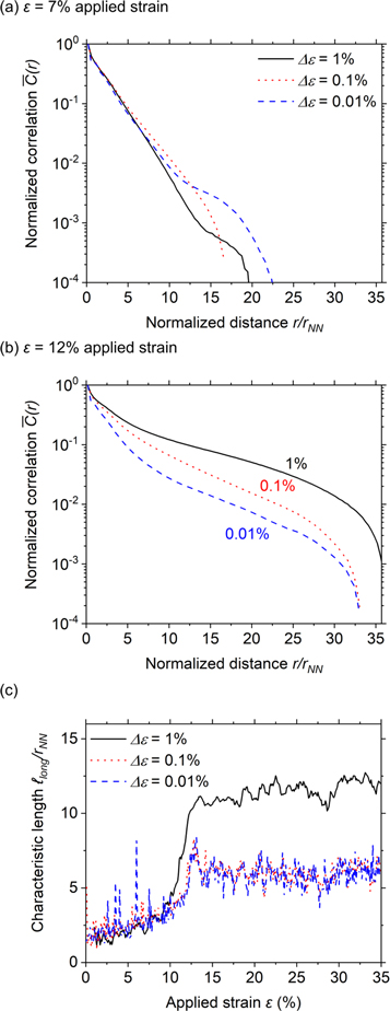
Figure 6. Auto-correlation functions of D2min calculated for different strain windows △ε, at 7% (a) and 12% (b) strain. (c) Shows the characteristic length ℓlong derived from the correlations for the different strain windows. All results were obtained with rcut = 3 rNN.
Download figure:
Standard image High-resolution imageTo clarify the role of  on the calculation of the correlation length
  we further tested the influence on system size on the correlation functions. Figure 7(a) shows that before yield (applied strain
  ),
),  is independent of system size but that a clear size dependence develops when the material flows (figure 7(c),
  ). Plotting
  versus applied strain
  shows that the before yield
  is independent of size but after yield it depends on system size (figure 7(b)). Normalizing distance r or correlation length
  by system size collapses all data in the region where the amorphous solid flows (figures 7(c) and (d)).
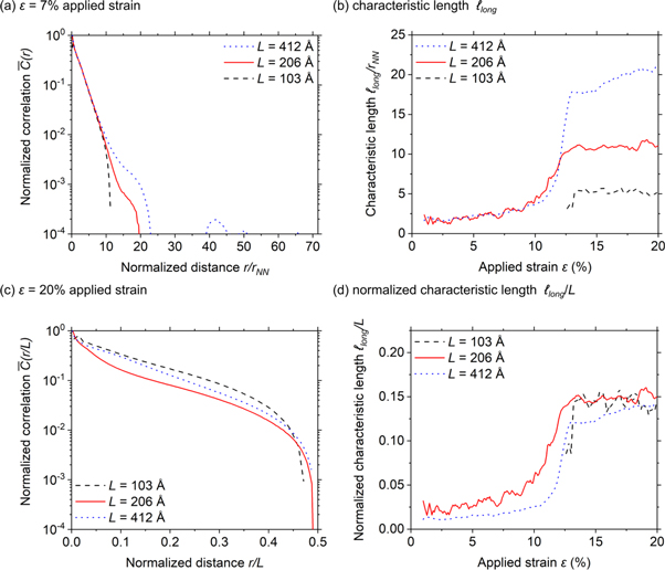
Figure 7. D2min auto-correlation functions for systems of different sizes, at 7% (a) and 20% (c) applied strain. (b) Shows the characteristic length ℓlong derived from the correlations for the systems of different size. (d) Shows the same curves as (b), but normalized with the system size L. All results are obtained with an offset Δε = 1% and rcut = 3 rNN. ℓlong curves for the small system with L = 103 Å start at ε = 11.9% because the data could not be fit to exponential over the range from 20 to 30 Å used to extract ℓlong.
Download figure:
Standard image High-resolution imageTo gain further insights into the system size dependence of  we took one of our medium-sized simulations at 20% applied strain and replicated it parallel (A) and perpendicular to the shear band (B, see insets in figure 8), creating simulation boxes with aspect ratios ≈2. We continued straining these 'supercell' systems up to 50% applied strain. System A continued to shear along the replicated shear band. System B had initially two shear bands, but one of the shear bands disappeared during shear in favor of the other, such that the final system had only a single shear band (inset in figure 8). While
  of system A remains unaffected,
  of system B rises to twice its initial value, like the cubic systems with twice the edge length.

Figure 8. Characteristic length ℓlong for as a function of the aspect ratio of the box for Δε = 1% and rcut = 3 rNN, but only for a single realization of the amorphous system (no averaging). The initial system was obtained by duplicating the size of a pre-strained system with a pre-existing shear band. Insets show exemplary maps of  for these two systems.
Download figure:
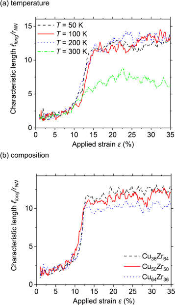
Standard image High-resolution imageFinally, we test the dependence of the correlation function on temperature and composition. Figure 9(a) shows the temperature dependence of  Data in the temperature range from 50 to 300 K, below the glass transition temperature of
  of our metallic glass, is superimposed for small strain. It appears that at large strain the highest temperature leads to a smaller
  while the values for the other temperatures are approximately the same. Figure 9(b) shows
  for different compositions. Again, the data collapses in the elastic regime and there appears to be a slight variation with composition after the sample has yielded.
Figure 9. Characteristic length ℓlong for (a) varying temperature and (b) varying composition. All results are obtained with an offset Δε = 1% and rcut = 3 rNN.
Download figure:
Standard image High-resolution image
4. Discussion
The correlation length  characterizing the exponential decay of the spatial-autocorrelation functions
  of
of  have in the past been interpreted as giving the size of the STZ [26]. Our results clearly show that the decay of
  with distance
  is exponential in MD calculations of BMGs, confirming other results obtained for EAM [26], Lennard-Jones [27] and hard-sphere glasses [29, 30]. However, there are two regions of exponential decay with different correlation lengths. At short distance
  the characteristic length
  is strongly affected by the choice of
  within which the non-affine part of the local deformation field is computed. Our results indicate
  such that
  does not characterize any intrinsic material scale. The initial decay crosses over to a second exponential at distances
  with a characteristic length
  that does not depend on the specific choice of
  and reference frame and is a characteristic of the material under investigation. For the CuZr glasses investigated here we find
  This is on the order of the values reported for FeP in [26]
  but smaller than the values for MgAl
  and CuZr
  reported there at an applied strain of
  for simulations carried out with an earlier version of the EAM potential used here [46]. Additionally, the work described in [26] used the initial configuration at
  as reference (and hence
  ) and looked at correlations of global non-affine displacements rather than
  Recent work using a Lennard-Jones model for CuZr reports
  [27]. This appears to indicate that the actual value of the correlation length is highly model-dependent and may also depend on the preparation of the glass. As an extreme example, for a poorly tempered system that does not show shear bands, we would not expect the correlation length to increase suddenly and become system size dependent at the onset of yield. For our systems, we find that the values extracted from our calculations are robust to variations of temperature and stoichiometry.
The situation in the pseudoelastic regime before yield is characterized by individual regions of large  (figure 1(b)) that are typically attributed to individual STZs. Therefore,
  measures the autocorrelation of the deformation field of an individual STZ. Since the overall density of STZs is low, the strain offset
  that determines over how many STZs we average does not affect the results. The situation changes dramatically after the sample has yielded (
 ). STZs are now localized within a shear band and it becomes difficult to identify individual STZs (figures 3(c) and (d)). The onset of shear-banding is then accompanied by a characteristic length
  proportional to the system size
  that depends on strain window
  For strain windows smaller than the cage-breaking strain,
  we find values for
  comparable to the ones found in the elastic regime (figure 6(c)). This is because even for the flowing glass with a shear band we can identify individual STZs if we look at small enough strain windows. Figures 3(e) and (f) show examples of the distribution of regions of large
  for
for  that clearly show individual STZs. The correlation length
  computed for
  therefore, like in the pseudoelastic regime, characterizes the size of an individual STZ rather than the correlation along the shear band. Note that Cubuk et al [32] have chosen to evaluate
  at a value of
  that corresponds to the minimum in the
  behavior obtained during flow of the material. Figure 6(c) indicates, that
  for
for  and a system size dependence for
  in our calculations. Cubuk et al are therefore likely in the region where
  They find exponential correlation in all cases and their extracted scale is independent of analysis protocol and system size.
The actual value of  depends on the size perpendicular to the shear band. Our 'supercell' calculations show that duplicating a shearing simulation (with an existing shear band) parallel to the shear band (system A in figure 8) does not affect
  while duplicating it perpendicular to the shear band (system B in figure 8) also doubles
  Note that in the latter case only one of the two shear bands survived during consecutive strain. The scaling
  is therefore simply a consequence of the ratio between the volume occupied by the band (it is of a thickness on the order of the size of the STZ that does not depend on system size) and the cell volume, or in other words,
  measures the distance between individual shear bands in the superlattice of shear bands created by the periodic boundary conditions. For an experimental system of a size much larger than the STZ size, this length scale would look divergent.
We would like to note that our system sizes, although large, are yet too small to rule out power-law behavior during flow. Indeed, the fact that for  our length scale
  depends on system size for is indicative of a diverging length scale. This could be a signature of a cross-over to a power-law as STZ events become correlated within the shear band. This observation is consistent with a recent proposition that yield in amorphous solids can be interpreted as a first-order phase transitions [47, 48], an interpretation that has a rich history for explaining shear-banding instabilities in non-Newtonian fluids [49]. Jaiswal et al [47] identified the transition using an order parameter that measures similarity or 'overlap' of atomic configuration. The atomic configuration loses overlap with the initial configuration at yield. A central observation is that their 'yield' point occurs at larger strains than the overshoot in the stress–strain curve that is typically attributed to yield. This is consistent with our calculations, which show that
  rises after the stress has peaked. As a guide to the eye, the gray vertical band in the stress–strain curve (figure 3(a)) indicates the applied strain where
  rises rapidly (see also figures 7(b), (d)).
We note that power-law correlations can be found in other measures for the non-affine displacement field rather than  for example by looking at the global non-affine displacement field rather than at the non-affine displacements in augmentation spheres of radius rcut as employed for the computation of
  In the elastic regime, the displacement-difference correlation function of a disordered body shows power-law behavior that describes the elastic Green's function [50, 51]. In the plastic regime, power-law scaling persists albeit with a different exponent that is compatible with a self-affine geometry for the deformation field [35]. Similar scaling has been observed for correlation of the strain field [34]. However, this type of scaling cannot be detected in the bare correlation function of the non-affine displacement (only in the difference correlation); and it appears to be not manifested in the local deviation from affinity as described by
5. Summary and conclusion
We studied the correlation between non-affine displacements, as characterized by the  measure of Falk and Langer [15], using MD calculations. This multipoint correlation function shows exponential behavior in the elastic regime from which we can extract a length scale
  typically attributed to the size of an STZ. We find that this length scale diverges at yield, as manifested by a size-dependent
  in during flow of the material. The divergence of
  occurs at strains larger than the peak stress that is typically attributed to the yield point. Our results support a recent proposition that yield in amorphous materials can be interpreted as a first-order phase transition [47, 48].
Acknowledgments
We thank Suzhi Li and Jan Mees for useful discussion and the Deutsche Forschungsgemeinschaft (DFG) for funding this work through grant PA 2023/2. All simulations were conducted with LAMMPS [52] on JURECA at the Jülich Supercomputing Center (grant 'hfr13') and on NEMO at the University of Freiburg (DFG grant INST 39/963-1 FUGG). Post-processing and visualization was carried out with ASE [53], matscipy [54] and Ovito [55].
Appendix. Calculation of the spatial correlation in reciprocal space
Appendix.
Spatial correlations can be computed straightforwardly by implementing equation (2) directly, with the  -function broadened into discrete bins. This calculation, however, becomes prohibitive for large distances, since the number of pairs of atoms scales with the distance squared. In order to speed-up the calculation (for large distances), we map our field Q onto a regular grid

where x, y and z are integers denoting points on a grid of NDFT = NxNyNz grid points. We chose Qx,y,z;i = Qi for  closest to the position of atom i,
  and zero otherwise. Other choices like a Gaussian interpolation or a distribution over all neighboring grid points are possible, but not used here. They only affect the results at small distances. Note that
  are the cell vectors that describe the tilted cell.
The discrete Fourier transform, and the inverse transform, of Qx,y,z are given by


with  The autocorrelation map in reciprocal space is obtained from the transform of equation (2)

which in real space yields

The tilt of simulation box is accounted for automatically, by using the appropriate cell vectors in the Fourier transformation. Specifically, the phase of equations (9) and (10),  where
where  are the reciprocal lattice vectors. Our reciprocal lattice vectors are normalized such that
  Care needs to be taken that when computing radial averages of
 ,$](https://content.cld.iop.org/journals/2515-7639/2/4/045006/revision2/jpmaterab36edieqn200.gif) the tilt of the box vectors is appropriately accounted for.
the tilt of the box vectors is appropriately accounted for.
The periodic boundaries of the system, in reciprocal space, also pose no problem as all pairs of grid points at a certain (real space) distance one from another collapse onto the same reciprocal grid point. Note that the fidelity of the autocorrelation at short distances depends on the choice of the size of the grid and the interpolation prescription. We here use  for the radially averaged correlation functions and use
  for the correlation maps shown in figure 4. We systematically checked implementation of equation (12) against a brute-force estimate of equation (2) to check that as
  we obtain the brute force estimate at short distances. We have implemented this algorithm in matscipy [54] and Ovito [55] and it is available in the public repositories of these codes.