

Abstract
As a result of planetary heating, global mean sea level has increased since the end of the 19th century. Sea level rise is accelerating and will continue to rise over the 21st century and beyond. On top of the global mean signal there are large regional variations in the magnitude of sea level rise. At a local level, reliable projections of probable and possible future sea level change are vital for coastal management planning. In this work we present an observational analysis of recent sea level variations at locations around the coast of South Africa using tide gauge records and satellite altimetry data. In recent decades, sea level around South Africa has increased at a rate of around 3 mm year−1, consistent with estimates of global mean sea level rise over that time. We apply existing methods (that are rooted in the methods of the 5th Assessment Report of the Intergovernmental Panel on Climate Change, but with a number of methodological innovations) to produce sea level projections for eight locations around the coast of South Africa under low (RCP2.6) and high (RCP8.5) emissions scenarios. In the year 2100 locations around South Africa are projected to experience sea level rise (relative to 1986–2005) of approximately 0.5 m (0.25–0.8 m) following RCP2.6, or around 0.85 m (0.5–1.4 m) following RCP8.5. These increases are around 7%–14% larger than projections of global mean sea level, due to the local amplification of increases in several components of the sea level budget. The results from this work suggest that successful mitigation efforts to reduce greenhouse gas emissions would have a clear benefit in limiting 21st century sea level rise for South Africa.
Export citation and abstract BibTeX RIS

Original content from this work may be used under the terms of the Creative Commons Attribution 4.0 licence. Any further distribution of this work must maintain attribution to the author(s) and the title of the work, journal citation and DOI.
1. Introduction
Quantifying and responding to current and future impacts of sea level rise on coastal environments is a key challenge faced by society. By the end of the 21st century the risks of erosion, flooding and salinisation are very likely to significantly increase along all low-lying coasts (IPCC 2019). Numerous studies have shown that on century timescales, mean sea level (MSL) rise is the primary driver of projected changes in extreme sea levels and the associated coastal flood risk (e.g., Cannaby et al 2016, Vousdoukas et al 2018, Howard et al 2019). The IPCC Special Report on Oceans and Cryosphere in a Changing Climate (SROCC) states that extreme sea level events that were historically rare will become common by 2100 under all radiative forcing scenarios considered (Oppenheimer et al 2019). For the purposes of risk assessment, coastal management and adaptation planning, reliable projections of future sea level rise at a local level are therefore vital.
While the physical character of the South African coastline may make it less vulnerable to sea level rise than neighbouring Mozambique or other African countries such as Egypt, it has a large urban population in the coastal zone relative to other countries on the continent, with relatively large projected costs for adaptation (Hinkel et al 2012, El-Shahat et al 2021). The eastern coast is characterised by sandy beaches with low coastal plains that are vulnerable to flooding and erosion caused by cyclonic weather events and associated large waves, locations with urban coastal development are particularly vulnerable, with Durban being a key example (Mather and Stretch 2012). The rocky shorelines around the Western and Eastern Cape regions are less vulnerable, although the estuaries and tidal inlets in these areas, many of which have residential or industrial developments, are likely to be at some risk (Hughes et al 1993, Mather and Stretch 2012). As well as an understanding of current sea level trends and variability, projections of future sea level rise are needed to inform coastal planning and adaptation strategies.
In the global mean, changes in MSL (the time-mean height of the sea surface, averaging over short-term fluctuations due to tides, waves and surges) occur through thermal expansion, melting of land-based ice and changes in land water storage (IPCC 2019). The change in MSL felt in any local region is driven by several factors, and their combined effect can lead to local sea level rise that is larger or smaller than the global average. As well as the influence of gravitation, rotation and deformation (GRD) that locally alter the contribution from mass input terms (see section 2.4) and the effects of ongoing glacial isostatic adjustment (GIA; see section 2.5), local changes in ocean circulation and density play an important role. South Africa is uniquely situated at the junction of the South Atlantic, Indian and Southern Oceans, with the Agulhas Current off its eastern and southern shores bringing warm and saline waters to the region. The strong westerly winds over the Southern Ocean play a major role in regional ocean dynamics. Under climate change, the westerlies have strengthened and shifted poleward, associated with a positive trend in the Southern Annular Mode (SAM; Thompson and Solomon 2002), and these changes are expected to continue (Swart and Fyfe 2012). One of the effects of these changes in the westerlies is a dipole in Southern Ocean sea level rise, being larger than the global average north of 50°S and smaller to the south (Bouttes et al 2012). At a broad level, these changes put the coast of South Africa in a latitude band of enhanced sea level rise. Studies on future changes in the Gulf Stream suggest that its projected weakening (associated with a decline in the Atlantic Meridional Overturning Circulation, AMOC) will cause enhanced sea level rise along the eastern coast of North America (Yin et al 2009). In contrast, the influence of the meridional overturning does not apply to the Agulhas Current, though recent studies have explored possible effect of changes in wind stress. Some suggest that Agulhas Current may strengthen as a result of increased SAM (Yang et al 2016), but others suggest a weak relationship with the SAM (Elipot and Beal 2018). Beal and Elipot (2016) suggest that the strengthening winds have caused the Agulhas current to become broader with more intense eddy activity, rather than a strengthening of its mean flow.
In this paper we present a new observational analysis using improved tide gauge records and multiple satellite altimeter datasets to establish the current rates of sea level rise around the coast of South Africa. We then apply the sea level projection methods of Palmer et al (2020) to several tide gauge locations around South Africa to calculate projections for sea level rise over the 21st century. These methods are rooted in the projections presented in AR5 (Church et al 2013), with a number of methodological advancements. These include: (i) updated and scenario-dependent treatment of projected mass loss from Antarctica from ice dynamics processes, following Levermann et al (2014); (ii) improved treatment of local projection uncertainties using a Monte Carlo framework; (iii) a regression/pattern-scaling approach to local ocean dynamic sea level change that better isolates the forced response from simulated internal variability. Further details are available in Palmer et al (2018, 2020). Overall, the global and local sea level projections obtained via this method are similar to those presented in the SROCC (Oppenheimer et al 2019).
In section 2 we outline the observational and model data used in this study. Section 3 summarises the sea level projections method which is described in more detail by Palmer et al (2020). In section 4 we examine recent sea level trends for South Africa from tide gauge and satellite altimetry observations. Future sea level projections for the 21st century at South African locations are presented in section 5. Conclusions and further discussion are given in section 6.
2. Data
2.1. Tide gauge data
Observational records of MSL at eight tide gauge stations around the coast of South Africa were obtained from the Permanent Service for Mean Sea Level (Holgate et al 2013, PSMSL 2020) with permission from the National Hydrographer of the South African Navy Hydrographic Office (SANHO). Tide gauge stations were selected based on the temporal range of their available records and to span the geographic domain. We used the Revised Local Reference (RLR) dataset, as this contains the sites that have a full benchmark history. The tide gauge data have not been revised to remove the estimated effect of glacial isostatic adjustment (GIA); this allows consistency with the model projections, which include GIA estimates (see section 3). The PSMSL has relatively strict criteria for computing annual MSL values (individual years must have at least 11 months of measurements with at least 15 days of records for each month), which greatly restricts the length of time series available for annual time series analysis. As the seasonal variations in MSL around the coast of South Africa are small, we applied less strict criteria for calculation of annual data from the available monthly data, including at first, all months that contain MSL values, irrespective of the number of missing days. We then undertook our own quality control procedures, as it was obvious the data contained erroneous monthly values. We used the 'buddy gauge' method of comparing nearby records of monthly or annual MSL, which is useful for catching datum shifts in records (e.g., Hogarth 2014, Hogarth et al 2020) and other errors. Using this approach, and expert judgment, we removed obvious monthly outliers. For example, records at a number of sites (Port Nolloth, Knysna, Port Elizabeth and East London) contained a large step change in monthly MSL for the second half of 2002. From the magnitude of change we suspect this is most likely associated with an uncorrected datum change, and not a real oceanographic process, and hence we removed the values in this period for these stations. We then calculated annual means for MSL at tide gauge stations from the available monthly mean data, after removing erroneous monthly values.
2.2. Satellite altimetry data
Observed sea surface height data are taken from three satellite altimetry products. Each of the products use data from multiple satellite missions which are reprocessed, homogenized and available on a 2D grid. The three products are as follows.
- The CMEMS product is produced and distributed by the Copernicus Climate Change Service (C3S) and is designed for the monitoring of long-term evolution of sea level. It is provided on a ¼ × ¼° latitude-longitude grid, and the dataset used in this study spans the years 1993–2018. Data are available from https://resources.marine.copernicus.eu/?option=com_csw&view=details&product_id=SEALEVEL_GLO_PHY_CLIMATE_L4_REP_OBSERVATIONS_008_057
- The ESA-CCI product is v2.0 of the European Space Agency (ESA) Climate Change Initiative for observations of sea level (http://www.esa-sealevel-cci.org; Legeais et al 2018). The dataset spans the years 1993–2015 and is provided on a ¼ × ¼° latitude-longitude grid.
- The CSIRO product is available from https://www.cmar.csiro.au/sealevel/sl_data_cmar.html. It is provided on a 1° × 1° latitude-longitude grid. The dataset used in this study is the one without the inverse barometer and GIA corrections applied and spans the years 1993–2018.
Each dataset is provided as monthly means, which we convert to annual means. For each tide gauge station in figure 1 a time series of sea surface height is extracted at the nearest ocean grid point to its latitude-longitude coordinate. We note that apart from the lower spatial resolution of the CSIRO product, we know of no evidence to suggest that any one of the three altimeter products is more appropriate than any other for the purpose of monitoring regional sea level around South Africa. We make use of all three products, whose different processing decisions provide some idea of uncertainty.
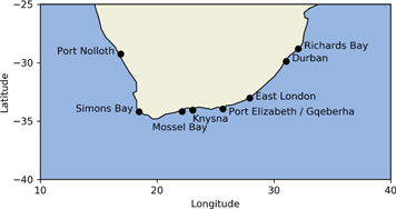
Figure 1. South African tide gauge locations used in this study. These eight locations were chosen based on length of record on PSMSL web data portal and to span the geographic domain. The city of Port Elizabeth was renamed Gqeberha in February 2021.
Download figure:
Standard image High-resolution image2.3. CMIP5 data
We use data from 21 CMIP5 model simulations (Taylor et al 2012) for the 21st century (2007–2100) with radiative forcing following two Representative Concentration Pathway (RCP) climate change scenarios (Meinshausen et al 2011): RCP2.6 (low radiative forcing, approximately equivalent to a global surface temperature increase of 1.5 °C above pre-industrial levels by 2100) and RCP8.5 (high radiative forcing, approximately equivalent to an increase of 4.5 °C by 2100). For context, RCP2.6 is the scenario most consistent with the Paris Agreement, but recent studies suggest that the world is most likely to follow a pathway in between these two scenarios, with an increase of around 3 °C by 2100 (Hausfather and Peters 2020). A list of the CMIP5 models used for the 21st century projections is given in table S4 in supplementary material (available online at stacks.iop.org/ERC/4/025001/mmedia).
The ocean components of CMIP5 models have a typical spatial resolution of 1° (equivalent to approximately 100 km in midlatitudes). Distances between the tide gauge stations in figure 1 are greater than this, with the exception of the distance between Mossel Bay and Knysna (which is approximately 85 km). When data is taken from the nearest grid box to each station location (see section 3), the grid boxes used for Mossel Bay and Knysna are unique in all except three of the 21 models used. However, the relatively coarse spatial resolution of CMIP5 models means it is not possible to fully resolve sharp gradients and the magnitude of dynamic sea level change is likely to be underestimated. Dynamical downscaling can be used to obtain dynamic sea level projections at much higher resolution and recent studies suggest that this underestimate in 21st century changes could be of the order of 10 cm in places, although the largest discrepancies are not generally found very close to the coast (Liu et al 2016, Zhang et al 2017, Hermans et al 2020).
Time series of global mean thermosteric sea level (model variable name zostoga), which is also referred to as global thermal expansion (GTE), are drift corrected as in Palmer et al (2020). These are used to calculate the global mean sea level projections along with global mean surface temperature (GMST, model variable name tas), which is used in the calculation of some barystatic sea level components (see section 3). For the local projections at locations around South Africa we make use of the 2D ocean dynamic sea level variable (zos), extracting its time series at the nearest ocean grid point to the latitude and longitude coordinate of each tide gauge station. This is used to establish the local linear regression relationship between global thermal expansion and local sterodynamic sea level change as described in section 3 and in more detail by Palmer et al (2020).
2.4. GRD estimates
The contributions from the barystatic (mass input) components vary spatially due to their effects on Earth's gravity, rotation and solid earth deformation. Following the nomenclature of Gregory et al (2019), we refer to these as GRD (gravitation, rotation and deformation) effects. Following Palmer et al (2020) we use three estimates for the spatial GRD patterns associated with the ice mass terms: Slangen et al (2014), Spada and Melini (2019), and Klemann and Groh (2013). The latter is extended to include rotational deformation following Martinec and Hagedoorn (2014). Following Slangen et al (2014), we use one estimate for the GRD pattern associated with land water storage (Wada et al 2012). The GRD estimates are expressed as the change in local MSL per unit change in GMSL. More details of the GRD calculation are provided by Palmer et al (2020).
For the eight locations around the coast of South Africa, the mean of the three GRD estimates (or the single land water estimate) are given in table 1, with the range showing the variation across the eight tide gauge locations around the coast. For all components except Antarctic surface mass balance, the GRD estimates are greater than unity, meaning that the mass input to the ocean has a greater effect on local MSL in South Africa than it does in the global average. The effect of changes in land water storage has a particularly large proportional effect on South Africa, although the absolute contribution from land water storage change is small (see section 5). Since the mass loss from ice sheets is associated with a near-field fall in MSL and a larger rise in the far-field, the Greenland components have a larger relative effect for South Africa than those from Antarctica (Tamisiea and Mitrovica 2011). This can be seen in the spatial GRD patterns shown in figure 3 of Palmer et al (2020), which are the same as used in the present study.
Table 1. GRD estimates for each barystatic sea level component. The values are the mean of three GRD estimates (one for land water) as described in the text, expressed as a percentage of each component's contribution to GMSL. The range is that spanned by the eight tide gauge locations around the coast of South Africa (see section 2.1).
| Barystatic sea level component | GRD range for South Africa tide gauge locations (% of global mean) |
|---|---|
| Antarctic ice dynamics | 111%–117% |
| Antarctic surface mass balance | 92%–97% |
| Greenland ice dynamics | 119%–127% |
| Greenland surface mass balance | 118%–125% |
| Glaciers | 109%–111% |
| Land water | 122%–134% |
2.5. GIA estimates
The relative sea level change experienced at the coast is affected by vertical land movement as well as local changes in sea surface height. A key process that drives vertical land movement is glacial isostatic adjustment (GIA), which is the ongoing adjustment of the lithosphere and viscous mantle material due to past changes in ice loading (e.g., Tamisiea and Mitrovica 2011). The associated changes in mass distribution also drive changes in Earth's rotation and gravity field, with further impacts on local sea level. Following Palmer et al (2020), we use three estimates of the influence of GIA on sea level, each on a 1 × 1° grid. The first two, ICE-5G (VM2 L90) (Peltier 2004) and ICE-6G_C (VM5a) (Argus et al 2014, Peltier et al 2015) were both obtained from http://www.atmosp.physics.utoronto.ca/%7Epeltier/data.php. The third estimate is from the Australian National University based on an update of Nakada and Lambeck (1988) in 2004–2005. Since the time scales associated with GIA effects are thousands of years, we set the GIA rates to be fixed at their present-day estimated values. For the eight tide gauge locations around South Africa (section 2.1), the mean of the three GIA estimates ranges from −0.21 mm yr−1 to −0.32 mm yr−1, indicating that GIA provides a small negative contribution to sea level rise in this region. Additional processes, including plate tectonics, sediment compaction, volcanic activity and anthropogenic influences such as groundwater extraction can also affect local vertical land motion (e.g, Wöppelmann and Marcos 2015). These processes are not included in this study but are an important consideration for local decision-making.
3. Sea level projections method
21st century sea level projections were produced as part of the IPCC AR5 (Church et al 2013) and SROCC (Oppenheimer et al 2019) using data from CMIP5 model simulations under RCP emissions scenarios. For this study we use the methods described by Palmer et al (2020) and used in the UK national climate projections (Lowe et al 2018, Palmer et al 2018), which built upon the science of AR5 and SROCC with a number of innovations. These include more comprehensive treatment of uncertainties and direct traceability between global and local projections; the local projections preserve the underlying correlation structure in the GMSL Monte Carlo simulations (see below), whereas AR5 and SROCC made statistical approximations to derive regional uncertainties. The contribution from Antarctica has also been updated relative to AR5 (see below). Full details are available from Palmer et al (2020), but a summary of the method is provided here for convenience.
The first step is the calculation of GMSL projections, which comprise contributions from seven physical components: global mean thermodynamic sea level, Antarctic mass balance, Antarctic ice dynamics, Greenland surface mass balance, Greenland ice dynamics, glaciers, and land water storage. Global mean thermodynamic sea level is obtained directly from the zostoga model variable and, unlike the other components, does not involve a change in ocean mass. The surface mass balance terms for Antarctica, Greenland and worldwide glaciers are estimated from time series of GMST (tas) using simple models (Church et al 2013). The ice dynamics terms are scenario-dependent but do not use CMIP5 data. Following Palmer et al (2020), in a departure from Church et al (2013), the contribution from Antarctic ice dynamics is parameterised using the scenario-dependent scaling of Levermann et al (2014). The contribution from Greenland ice dynamics is estimated as a quadratic function of time with scenario-dependent final value (Church et al 2013). Net changes in land water storage are assumed to be independent of scenario and modelled as a quadratic function of time (Church et al 2013).
For each component there is a distribution of time series to capture the underlying uncertainty. The CMIP model-based terms use the spread of the simulations, and larger Monte Carlo ensembles are constructed from these with the same mean and standard deviation and with correlations between GTE and GMST preserved. For each emissions scenario, the components are combined to obtain projections of GMSL by constructing a 450,000-member Monte Carlo simulation, with each member consisting of a set of time series of the seven sea level components, each sampled from its underlying distribution. As shown by Palmer et al (2020), projections of GMSL are very similar to those in AR5 and SROCC.
The GMSL projections are then used to obtain local sea level projections at tide gauge locations around South Africa. Additional processes need to be considered at the local level. The local influence of GRD effects on the MSL change associated with each of the mass input terms (section 2.4) is included, as well as the local influence of GIA (section 2.5). The effect of local changes in ocean density and circulation are included by using the linear regression relationship between GTE (zostoga) and local sterodynamic sea level change (zos+zostoga) in the CMIP5 model ensemble (a list of the 21 models used for this purpose is given in table S4 in supplementary material). The regression coefficient corresponds to the offset between the contribution from thermal expansion to GMSL change and the contribution from sterodynamic component to local MSL change. This 'pattern scaling' approach to sterodynamic sea level results in much smoother projections that better isolate the forced response from internal variability (Palmer et al 2020). The mean of the regression coefficients across the CMIP5 ensemble is greater than one for all the locations around South Africa (table 2), meaning the local oceanographic processes act to amplify the global sea level rise signal. The relative contribution from changes in local sterodynamic sea level is slightly lower under the high emissions scenario. This difference is may at least partly be due to a limitation in the linear regression approach. Figure S3 (supplementary material) suggests there may be some degree of nonlinearity at high GTE under strong emissions in some models (see also Bilbao et al 2015). Yuan and Kopp (2021) have recently proposed an improved method using a two-layer emulator that can capture the nonlinearities that are important in the centuries beyond 2100. However, figure S3 (for Durban, and equivalent figures for other locations, not shown) indicate that overall, a linear regression describes the relationship between local sterodynamic sea level and GTE through the 21st century very well.
Table 2. Mean and standard deviation across the 21 CMIP5 models of the linear regression coefficient between the change in global thermal expansion (zostoga) and the change in local sterodynamic sea level (zos + zostoga) over the 21st century. A regression coefficient greater than one indicates that the global sea level rise signal is locally amplified by changes in ocean circulation and/or density.
| Mean of regression coefficients | Standard deviation of regression coefficients | |||
|---|---|---|---|---|
| Location | RCP2.6 | RCP8.5 | RCP2.6 | RCP8.5 |
| Port Nolloth | 1.16 | 1.09 | 0.11 | 0.12 |
| Simons Bay | 1.22 | 1.08 | 0.13 | 0.14 |
| Mossel Bay | 1.20 | 1.06 | 0.14 | 0.17 |
| Knysna | 1.21 | 1.07 | 0.15 | 0.16 |
| Port Elizabeth/Gqeberha | 1.25 | 1.14 | 0.14 | 0.15 |
| East London | 1.28 | 1.18 | 0.15 | 0.15 |
| Durban | 1.18 | 1.05 | 0.23 | 0.23 |
| Richards Bay | 1.24 | 1.11 | 0.18 | 0.16 |
Local projections are obtained by performing a 150,000-member Monte Carlo simulation, drawing at random: (i) a member of the GMSL Monte Carlo; (ii) the sterodynamic regression coefficient at that location from one of the 21 CMIP5 models; (iii) the local amplification value from one of the three GRD estimates (or one in the case of land water); (iv) a contribution due to GIA from one of the three estimates. Before the resulting projections for the eight locations around South Africa are presented in section 5, we first put this into context by examining the observational data for sea level variations in these locations over recent decades.
4. Observed sea level rise at locations around South Africa
Recent variations and trends in sea level can be found in tide gauge records and sea surface height observations from satellite altimetry. These two observational types do not measure precisely the same sea level changes; they provide different and complementary information. Tide gauges (section 2.1) measure relative sea level variations with vertical land motion included, which is potentially the most impact-relevant for coastal locations, as long as the recorded land motion is real (not an artifact of events such as the repositioning of an instrument). Altimeter observations (section 2.2) measure geocentric sea level relative to Earth's mass, and do not include any contribution from vertical land motion. Altimetry provides valuable information at global and regional scales, but its accuracy can be diminished near the coast (Vignudelli et al 2011).
Time series of MSL from each tide gauge location and the altimeter data from the nearest grid point in the three gridded products are shown in figure 2. A comparison of linear trends calculated from tide gauge and altimeter observations in the overlapping period of 1993–2018 shows generally good agreement (figure 2, 3). The rate of sea level rise over the period 1993–2018 from altimeter observations is within 2–4 mm year−1 around the coast of South Africa, comparable with the value of 3.2 mm/year for global mean sea level rise over 1993–2015 reported by the SROCC (Oppenheimer et al 2019) (see also figure 7). From the altimeter data in figure 3 larger and smaller rates can be seen further offshore associated with mesoscale features, particularly in the Southern Ocean. These large values are not generally seen near the coast, which (bearing in mind the expected reduction in reliability in altimeter data here) is to be expected as baroclinic eddy features decay as they approach the coast (Zhai et al 2010). Rates of sea level rise over 1993–2018 from tide gauge records are also within 2–4 mm year−1 (or close; the rate at Simons Bay is very slightly larger at 4.2 mm year−1), with two exceptions. Records at Mossel Bay suggest a significantly larger rate of sea level rise (9.9 mm/year) since 1993, which appears to be associated with multidecadal variations of unknown origin at this location (figure 2). The PSMSL tide gauge documentation states that unlike other South African tide gauge stations, which are protected by harbours, the Mossel Bay station is more exposed to open water influences. It is conceivable that its more exposed location may cause the Mossel Bay tide gauge station to exhibit different temporal characteristics to neighbouring locations. However, given that these large variations are not seen at this location in any of the three altimeter datasets (figure 2), it may be more likely that they stem from long-term quality control issues (perhaps relating to datum instabilities). Port Elizabeth (Gqeberha) has a very low rate of 0.4 mm year−1, which is partly attributed to missing data in the 1990s (extending the trend window back to 1980 increases the trend to 2.2 mm year−1).
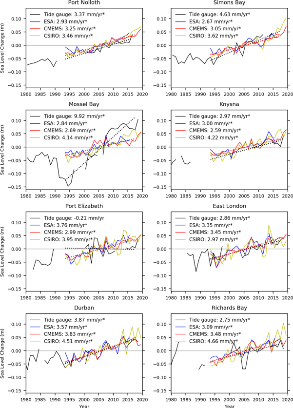
Figure 2. Time series of annual mean sea level data at each of the eight stations in figure 1 from tide gauges (black) and altimeter datasets from CMEMS (red), ESA CCI (blue) and CSIRO (yellow). Linear trends over 1993–2018 are shown in the legend for each time series, with an asterisk indicating trends that are significantly different from zero according to the 95% confidence interval from a two-sided inverse Student's t-distribution. Trend lines for tide gauges and the CMEMS altimeter only (for clarity) are included in the figure (black and red dotted lines respectively). Altimeter data are taken from the nearest grid box to the tide gauge location (see section 2.2).
Download figure:
Standard image High-resolution image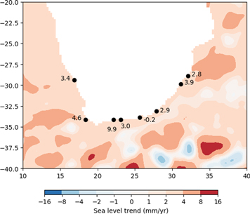
Figure 3. Rate of sea level rise from the CMEMS altimeter product 1993–2018. Equivalent figures for ESA-CCI and CSIRO altimeter products are similar and are shown in supplementary material (Figures S1 and S2). Numbers next to station locations show trends in tide gauge data in mm/year. The period over which tide gauge trends are calculated is the same as for the altimeter data (1993–2018), although the full range of years are not available for all tide gauge stations due to missing data (see figure 2).
Download figure:
Standard image High-resolution imageOverlying the long-term observed trends in MSL seen in figure 2 there is considerable interannual variability. The standard deviation of detrended annual mean MSL time series from tide gauge data and each of the three altimeter products are shown for each of the eight locations in table S1 in supplementary material. These results, along with figure 2, suggest that the variations at Port Nolloth are of smaller magnitude than at the other locations. This may be consistent with its location towards the northern part of the west coast of South Africa (figure 1), further from the dynamical influence of the Agulhas Current and its retroflection. In contrast to the projections for future MSL presented in the next section, which are designed to reveal the forced climate change signal, observations of MSL from tide gauges and altimetry provide records that contain the effects of various elements of internal climate variability. Previous studies have examined possible links between climate modes of variability and sea level at the coast of South Africa, including via their effects on the transport and position of Agulhas Current and hence absolute dynamic topography and coastal sea level. Elipot and Beal (2018) find that 29% of the interannual variance of the Agulhas Current transport can be related to modes of atmospheric variability, with the El Nino Southern Oscillation (ENSO) alone explaining 11.5%. However, they find that the SAM has no significant correlation with Agulhas transport. Nhantumbo et al (2020) explore links between modes of climate variability, the Agulhas Current and South African sea level variability. They find that the position of the Agulhas Current influences coastal sea level, with the extent of its influence varying between locations due to factors including the width of the continental shelf, location of the tide gauge and dynamics of the current. They find that on interannual time scales there are connections with ENSO, SAM and the Indian Ocean Dipole (IOD); the relationships are weak and not consistent between locations, but the general picture they find is that positive ENSO and IOD are associated with increased coastal sea level, while positive SAM is associated with reduced coastal sea level. Figure 2 reveals that while there is reasonably good agreement between the observational sources on the magnitude of the trends (at most locations; see above), there is little coherence of interannual fluctuations between the time series from tide gauges and altimetry. The detrended time series from the altimeter products are positively correlated, with particularly high correlations between the CMEMS and ESA CCI products (table S2 in supplementary), but a clear correlation between the altimeter and tide gauge time series is not found. The low and inconsistent correlations between South African sea level variations and ENSO (table S2 in supplementary material) also suggests that a clear connection to ENSO variability cannot be ascertained from this simple analysis; further exploration would require data at higher temporal resolution and is not the focus of the present study. In the next section we explore future projections for sea level around the coast of South Africa.
5. 21st century projections for tide gauge locations
For the eight tide gauge locations around South Africa we present the 21st century projections (2007–2100) calculated using the method described in section 3 (figure 4). The observed changes in sea level from tide gauge data (since 1970) and from the ESA CCI altimeter data (1993–2018) are also included to show the projected changes relative to the annual mean temporal variability seen in recent decades.
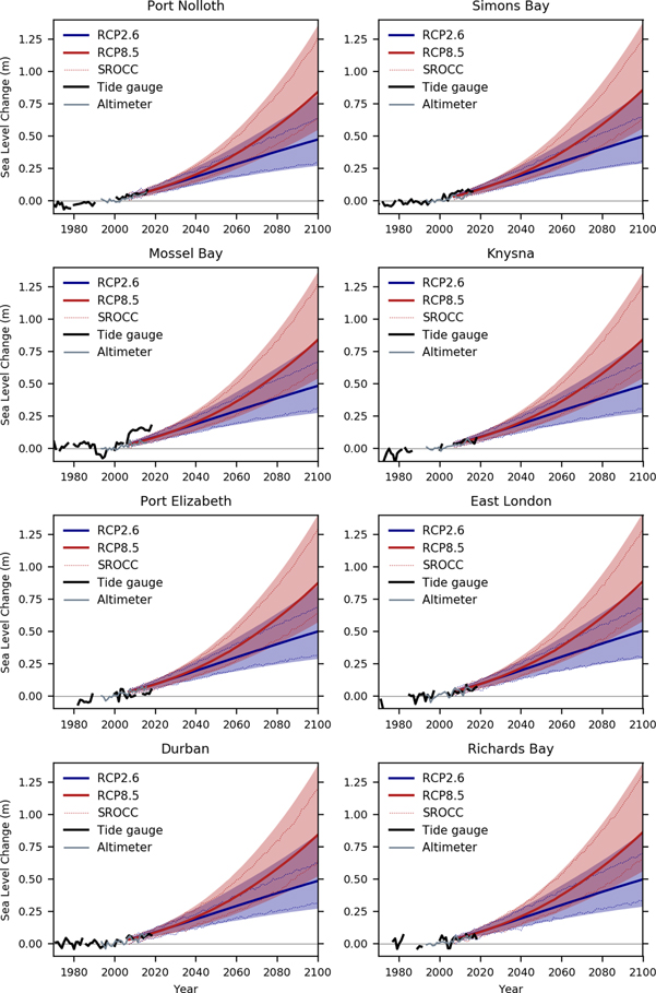
Figure 4. Projections of MSL change for the 21st century (2007–2100) for the eight South African tide gauge locations in figure 1. Shown are the projections for low (RCP2.6, blue) and high (RCP8.5, red) emissions scenarios. The solid lines show the median of the distribution of MSL projections, with the shading indicating the 5th-95th percentile range of the local Monte Carlo simulation. Annual mean values from the processed tide gauge data from 1970 (where available) are shown by the heavy black lines. Annual mean altimeter data from the ESA CCI product is shown in grey. The dotted coloured lines show the 5th and 95th percentiles for each emissions scenario from the IPCC SROCC projections (Oppenheimer et al 2019) for comparison. Each time series is presented relative to a baseline period of 1986–2005.
Download figure:
Standard image High-resolution imageThe projections for the locations around South Africa are similar; we show them all for completeness and to compare the observational records alongside. A summary of the projected sea level rise at 2100 is given in table 3. At 2100, relative to the 1986–2005 mean, locations around South Africa are projected to experience MSL rise of approximately 0.5 m (0.25–0.8 m) following RCP2.6, or around 0.85 m (0.5–1.4 m) following RCP8.5 (with the numbers in parentheses indicating the 5th − 95th percentile range of the distribution). The time series in figure 4 indicate that the projected MSL rise following RCP2.6 is approximately linear, but there is a clear acceleration over the 21st century following RCP8.5.
Table 3. Summary of mean sea level (MSL) projections at 2100 (relative to a 1986–2005 baseline period) for locations around South Africa. The central estimate and the 5th–95th percentile range are given (in metres), along with these values expressed as a percentage of their global mean values. The contributions from each of the sea level components for Durban and the global mean are given in supplementary material (table S3).
| Central estimate, meters, and % of global mean central estimate in parentheses | 5th–95th percentile range, meters, and % of global mean percentile range in parentheses | |||
|---|---|---|---|---|
| Location | RCP 2.6 | RCP8.5 | RCP2.6 | RCP8.5 |
| Port Nolloth | 0.47 (107%) | 0.84 (108%) | 0.27–0.82 (115%) | 0.55–1.35 (114%) |
| Simons Bay | 0.50 (114%) | 0.86 (110%) | 0.29–0.84 (115%) | 0.56–1.38 (117%) |
| Mossel Bay | 0.48 (109%) | 0.84 (108%) | 0.27–0.83 (117%) | 0.54–1.36 (117%) |
| Knysna | 0.48 (109%) | 0.84 (108%) | 0.27–0.83 (117%) | 0.54–1.37 (119%) |
| Port Elizabeth/Gqeberha | 0.50 (114%) | 0.87 (112%) | 0.29–0.85 (117%) | 0.57–1.40 (119%) |
| East London | 0.50 (114%) | 0.89 (114%) | 0.29–0.86 (119%) | 0.58–1.42 (120%) |
| Durban | 0.49 (111%) | 0.84 (108%) | 0.27–0.85 (121%) | 0.52–1.38 (123%) |
| Richards Bay | 0.50 (114%) | 0.86 (110%) | 0.29–0.86 (119%) | 0.56–1.40 (120%) |
| Global mean | 0.44 | 0.78 | 0.27–0.75 | 0.53–1.23 |
As noted by Palmer et al (2020), the projections using this method are temporally smoother than those from the SROCC (dotted lines in figure 4), and with larger uncertainty ranges. The smoothness is likely due to the exclusion of residual variability in sterodynamic sea level in the underlying CMIP5 simulations; using the linear regression method better isolates the climate change signal. The larger uncertainty ranges here are primarily due to larger uncertainty in the contribution from Antarctica that emerges when using the scenario-dependent projections from Levermann et al (2014).
These results suggest that locations around South Africa are projected to experience higher sea level rise than is expected for the global mean (table 3), with the central estimates at the local stations being 7%–14% higher than the global mean. This is the case for both RCP2.6 and RCP8.5. A breakdown of the contributions from each component to the local projections for Durban and the global projections (table S3 in supplementary material) suggests that the larger sea level rise felt in South Africa (relative to the global mean) is driven by a larger increase in all the components except GIA which has a negative contribution.
The time-evolving contribution from each component to projected local MSL change at Durban is shown in figure 5. The results for other locations are similar (not shown). At this location, the largest contribution to MSL rise throughout the 21st century comes from the ocean sterodynamic component (contributing 37% or 40% of the total increase at 2100 for Durban under RCP2.6 and RCP8.5 respectively; table S3 in supplementary material), with glaciers and Greenland having the next largest contributions. The acceleration in total MSL rise seen for RCP8.5 is driven by an acceleration in the sterodynamic and Greenland components, with a smaller contribution from an acceleration of the contribution from glaciers.

Figure 5. Time series of contributions to projected sea level change at Durban for each component, for emissions scenarios RCP2.6 (left) and RCP8.5 (right). For clarity the 5th—95th percentile range is shown only for the total and the sterodynamic and net Greenland components. The contributions from Antarctica and Greenland (surface mass balance and ice dynamics) are combined here to show the net contribution from each of the ice sheets. The grey line is the horizontal axis (zero sea level change).
Download figure:
Standard image High-resolution imageThe contributions from each component to MSL change for the year 2100 (relative to 1986–2005) and their associated uncertainty is shown for three other South African locations and the global mean in figure 6. The largest uncertainty comes from the Antarctic component (the combined effect of surface mass balance changes and ice dynamics), and this component is also behind the positive skewness in the uncertainty range for the total MSL change. For Greenland, the uncertainty under RCP8.5 is more than double that under RCP2.6; its uncertainty under RCP8.5 increases sharply after around 2060 (figure 5).

Figure 6. Components of the sea level projection at 2100 for three tide gauge locations (Port Nolloth, west coast; Port Elizabeth/Gqeberha, south coast; Richards Bay, east coast) relative to the 1986–2005 baseline period. Lines indicate the central estimate for each component under RCP2.6 (blue) and RCP8.5 (red). The land water and GIA components are independent of emissions scenario and are shown in grey. For the global mean, GIA does not contribute, and the ocean component is due to thermal expansion only.
Download figure:
Standard image High-resolution imageThe uncertainty estimates are considerably larger at the local scale than for the global mean, particularly for the ocean sterodynamic component and total MSL. The 5th–95th percentile ranges for the two emissions scenarios are clearly distinct from one another for the thermal expansion component of global mean sea level change, but at the locations around South Africa, the ocean sterodynamic uncertainty ranges for the two scenarios overlap. The additional uncertainty in the sterodynamic component locally (over the thermal expansion globally) is partly due to the additional uncertainty in the ratio of the local sterodynamic effect (ocean dynamics and local steric effects) to thermal expansion; there is a distribution of CMIP5 regression coefficients about the mean (table 2). Additional uncertainty also arises due to the mean regression coefficient being greater than one (table 2), which causes the full distribution to be amplified by this factor, thus inflating the spread of the local distribution.
Relative to the sterodynamic component, uncertainty in the other components is amplified at the local scale to a lesser extent because the GRD patterns are less uncertain. There is a small amplification of the uncertainty caused by the inflation of the GMSL distribution when the GRD scaling values are greater than one, which is the case for all components except Antarctic surface mass balance (table 1). As discussed by Palmer et al (2020), we note that the GRD fingerprints do not account for changes in mass redistribution, meaning that there will be additional uncertainty not included here. Accounting for the changes in mass distribution would be a useful avenue for future research.
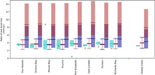
Despite the uncertainty in the projections, the difference between the estimates of MSL rise under the two emissions scenarios indicates that global climate change mitigation efforts would benefit locations around the coast of South Africa. Between RCP2.6 and RCP8.5 there is around a 70% increase in the central estimate and around a 75% increase in the 95th percentile. Figure 7 compares projected rates under each scenario with the recent observed rates of sea level change from available tide gauge and altimeter data. Rates over 1996–2018 from altimeter data are around 3 mm/year around South Africa, with tide gauge data generally in agreement but with some scatter (see also figures 2 and 3). Rates from the projections over 1996–2018 (the earliest years available) are generally in agreement with the observations within uncertainties. Under RCP2.6, long-term rates of sea level rise around South Africa over the 21st century are only slightly higher than recently observed (and projected) rates (reflecting the approximately linear sea level rise seen in figures 4 and 5 for RCP2.6). However, under RCP8.5 sea level around South Africa is projected to increase at a rate at least double this, with central estimates of 8 to 9 mm year−1. Under RCP8.5 the 21st century rates for the 95th percentile are around 14 mm year−1, which is around four times larger than the observed and projected rates for the recent period.
Figure 7. Comparisons of observed and projected rates of MSL rise for eight locations around the coast of South Africa and the global mean. Observed rates from satellite altimetry (1996–2018) are shown in cyan, with the line indicating the mean of the CMEMS, CSIRO and ESA-CCI products at each location and the shading indicating the 5th–95th percentile range from these products. Green crosses are rates from tide gauge data for the available years between 1996–2018 (noting that not all locations have complete data for this period; missing data in the 1990s partly explains the low value for Port Elizabeth/Gqeberha, see also figure 2). Projected rates over the period 1996–2018 are shown as lines (central estimates) and whiskers (5th–95th percentile range). Projected rates over 2007–2100 are shown as shaded boxes (5th–95th percentile range) with lines for central estimates. For all the projections data, RCP2.6 is shown in blue and RCP8.5 in red. The observed global mean sea level rate is taken from SROCC (Oppenheimer et al 2019) for 1993–2015 and shown in black.
Download figure:
Standard image High-resolution image
6. Conclusions and discussion
South Africa, like the global average, is already seeing the effects of planetary warming on sea level rise, with observed rates over 1993–2018 of around 3 mm year−1 from tide gauge and altimeter records for most locations around the coast, in line with observations of global mean sea level rise. Satellite altimeters measure geocentric sea level, whereas tide gauges observe relative sea level including any vertical land motion. Having these independent sea level observations is beneficial as they allow values to be cross-checked, and the differences in what they measure mean that some of the physical contributions to observed sea level rise could potentially be identified. Understanding the drivers of observed sea level change is an important factor in making useful projections of future changes. This type of analysis may require more temporally complete tide gauge records than are presently available, and the recovery of missing historical records would be beneficial. Independent estimates of vertical land movement (e.g., differential GPS stations collocated with tide gauges) would also be useful to help to disentangle the drivers of present-day sea level change, since there are several additional factors that affect local relative sea level measurements (Wöppelmann and Marcos 2015); we hope to motivate future studies that address this issue. In addition, sea level observations at higher temporal resolution are also needed to constrain return-level curves. For example, the UKCP18 report (Palmer et al 2018) shows large uncertainties in return period curves around the UK. Tide gauge records exhibit considerable interannual and in some cases decadal variability, and as illustrated for Simons Bay by Palmer et al (2020), sea level variability is likely to be an important modulator of observed local sea level rise in the coming decades.
To estimate future changes in sea level over the 21st century at locations around South Africa we have applied the methods of Palmer et al (2020) to calculate MSL projections for eight locations under low (RCP2.6) and high (RCP8.5) emissions scenarios. Locations around South Africa are projected to experience sea level rise (relative to 1986–2005) of approximately 0.5 m (0.25–0.8 m) following RCP2.6, or around 0.85 m (0.5–1.4 m) following RCP8.5. These increases are around 7%–14% larger than projections of GMSL. This larger increase in MSL for South Africa relative to the global mean is driven by changes in local ocean circulation and density, as well as a local amplification of the effects of mass input (from all barystatic sources except Antarctic surface mass balance) through the influence of gravitation, rotation and deformation (GRD). The relatively coarse resolution of CMIP5 models means that it is not possible to fully resolve sharp gradients in dynamic sea level and results from dynamical downscaling studies suggest that the magnitude of sterodynamic sea level changes could be of the order 10 cm larger than found here (Liu et al 2016; Zhang et al 2017; Hermans et al 2020). The methods of the present study estimate the combined effect of all components of the sea level budget with a comprehensive treatment of uncertainty. Further studies that apply downscaling methods around southern Africa to reveal more realistic patterns of sterodynamic change would complement these results.
The local sea level projections have larger uncertainty than GMSL projections. This is partly because of uncertainty in the relationship between global and local projections (such as the regression relationship between global thermal expansion and local sterodynamic change) and also because of the inflation of the global distribution by an amplification factor greater than one in regions that are predicted to have MSL rise larger than global mean. Uncertainty in the spatial patterns associated with GRD effects also contribute to larger uncertainty at the local level.
The results from this work suggest that successful mitigation efforts to reduce greenhouse gas emissions would have a clear benefit in limiting 21st century sea level rise for South Africa. Relative to RCP2.6, the higher emissions scenario of RCP8.5 leads to a 70% increase in the central estimate of sea level rise for South Africa and a 75% increase in the 95th percentile estimate.
Although these results are premised on CMIP5 under RCPs, recent studies suggest that the projections would be similar under CMIP6 and shared socio-economic pathways (SSPs). Lyu et al (2020) state that projections of dynamic sea level from CMIP5 and CMIP6 'exhibit very similar features and intermodel uncertainties'. Hermans et al (2021) show that the higher effective climate sensitivity exhibited by CMIP6 models does not translate into significantly higher GMSL projections at 2100; the central estimate for GMSL is found to increase by 2–3cm and the 95th percentiles by 3–7cm. However, there may be an increase in the rate of change towards the end of the century, meaning that a substantially larger GMSL rise beyond 2100 may be implied.
It is important to note that the methods used in this study, rooted in the methods of IPCC AR5, characterise the central part of the probability distribution for sea level projections. It is widely recognised that more information is needed to better understand the 'tail risk' for sea level projections, such as through exploring possible high-end scenarios (e.g., Stammer et al 2019). The potential for marine ice cliff instability (DeConto and Pollard 2016), for instance, is not included in this type of analysis and could lead to substantially larger sea level rise than estimated here (Edwards et al 2019; DeConto et al 2021). However, probabilistic estimates for this type of physical process are difficult to quantify. One way to deal with this type of uncertainty is to consider physically-based high-end narratives alongside these CMIP-based projections (Palmer et al 2018; Rohmer et al 2019).
An understanding of past and current sea level change and projections of future sea level rise are needed to inform coastal management practices around the world. The varied character of the South African coastline and local socio-economic considerations give rise to the need for individual regional responses to the future risk of coastal flooding. Progress is being made towards collating and disseminating information about future climate risks (e.g., the 'Green Book' online planning support tool for South Africa's urban centres; CSIR 2019). Municipal governments in South Africa are establishing methods for managing changing coastal risks (e.g., Colenbrander et al 2014). Adaptation measures are needed where the coastline is vulnerable, such as locations where there are urban beachfronts and coastal development, particularly along the sandy eastern coast (Mather and Stretch 2012). Developing improved sea level projections that take into account possible high-end scenarios would help to inform planning decisions at a local level.
Acknowledgments
This work and its contributors were supported by the Met Office Weather and Climate Science for Service Partnership (WCSSP) South Africa as part of the Newton Fund. Tide gauge data are provided with permission from the National Hydrographer of the South African Navy Hydrographic Office (SANHO) as supplier and copyright holder. The authors are aware that the tide gauge information contains gaps, and the South African National Hydrographer cannot be held responsible for the results obtained. We acknowledge the World Climate Research Programme's Working Group on Coupled Modelling, which is responsible for CMIP, and we thank the climate modelling groups for producing and making available their model output. For CMIP the U.S. Department of Energy's Program for Climate Model Diagnosis and Intercomparison provides coordinating support and led development of software infrastructure in partnership with the Global Organization for Earth System Science Portals. We are grateful to two anonymous reviewers whose insightful comments improved the manuscript.
Data availability statement
All data that support the findings of this study are included within the article (and any supplementary files).