

Abstract
Plug-in hybrid electric vehicles (PHEV) have an electric motor and an internal combustion engine and can reduce greenhouse gas emissions (GHG) from transport. However, their environmental benefit strongly depends on the charging behaviour. Several studies have analysed the GHG emissions from upstream electricity production, yet the impact of individual charging behaviour on PHEV tail-pipe carbon emissions has not been quantified from empirical data so far. Here, we use daily driving data from 7,491 Chevrolet Volt PHEV with a total 3.4 million driving days in the US and Canada to fill this gap. We quantify the effect of daily charging on the electric driving share and the individual fuel consumption. We find that even a minor deviation from charging every driving day significantly increases fuel consumption and thus tail-pipe emissions. Our results show that reducing charging from every day to 9 out of 10 days, increases fuel consumption on average by 1.85 ± 0.03 l/100 km or 42.7 ± 0.8 gCO2 km−1 tail-pipe emissions (± on standard error). Charging more than once per driving day has less impact in our sample, this must occur during at least 20% of driving days to have a noteworthy effect. Even then, a 10% increase in frequency only has moderate effect of decreasing fuel consumption on average by 0.08 ± 0.02 l/100 km or 1.86 ± 0.46 gCO2 km−1 tail-pipe emissions. Our results illustrate the importance of providing adequate charging infrastructure and incentives for PHEV users to charge their vehicles on a regular basis in order to ensure that their environmental impact is small as even long-range PHEVs can have a noteworthy share of conventional fuel use when not regularly charged.
Export citation and abstract BibTeX RIS

Original content from this work may be used under the terms of the Creative Commons Attribution 4.0 licence. Any further distribution of this work must maintain attribution to the author(s) and the title of the work, journal citation and DOI.
1. Introduction
Greenhouse gas (GHG) mitigation is strongly needed in the transport sector to limit global warming as stated in the Paris agreement. Plug-in hybrid electric vehicles (PHEVs) are plug-in electric vehicles (PEV) that can use electricity as well as conventional fuel for propulsion (Bradley and Frank 2009). Their potential to reduce local and global emissions strongly depends on their real-world usage and the share of kilometres driven on electricity, the so-called utility factor (UF) (Chan 2007, Jacobson 2009, Flath et al 2013). Thus, the actual environmental benefit of PHEVs strongly depends on usage, in particular charging (Plötz et al 2017a, 2017b, Plötz et al 2018, Srinivasa Raghavan and Tal 2020).
Currently, PHEV are one third of the global PEV fleet or about 9 million vehicles on the road (by the end of 2020) and still increasing (IEA 2021). PHEV are particularly relevant in Europe where they make up about half of current PEV sales. Furthermore, 133 PHEV models were offered globally in 2020 compared to 235 BEV models (IEA 2021) and the number of available models is still increasing. Thus, PHEV are both relevant in the current global PEV fleet and in terms of market shares in major vehicle markets. However, previous work has indicated insufficient charging of PHEV as a potential factor limiting the environmental advantage of PHEV.
Previous studies in the literature have analysed well-to-wheel GHG emissions but do not systematically study the effect of charging behaviour on tail pipe emissions. For example, Nordelöf et al (2014) as well as Kamiya et al (2019) focused on a life-cycle assessment of PHEV with fixed assumption on the share of kilometres driven on electricity. Likewise, IEA (2019) provided an update summary of the GHG intensity of battery production and electricity generation but did not go into detail about different PHEV charging behaviours (see section 1.1. for a brief overview of existing studies). Thus, the direct effect of PHEV charging on real-world tail pipe emissions has not been analysed in detail yet.
Here, we quantify the environmental effect of not charging a PHEV on some nights and the effect of charging a PHEV twice or more frequently per day, with a focus on the tail-pipe emissions of a long-range PHEV. More specifically, we analyse the change in utility factor (UF) —share of kilometres driven on electricity within total vehicle kilometres travelled (VKT) — and fuel consumption. While these measures are related, they capture different aspect of the environmental impact of PHEV. The UF is influenced by the total driving distance, while fuel consumption is directly related to the tail-pipe emissions of the PHEV.
This work differs from previous studies in several aspects. First, it is to our knowledge the first study that quantifies the effect of no overnight charging and additional charging empirically with a large sample. Second, while previous literature has looked at the impact of charging on the UF, the specific effect of charging frequency on fuel consumption and tail pipe emissions has not been analysed before. Third, our sample of real-world PHEV usage is quite large with a total of 7,491 PHEV and 3.4 million driving days; this allows us to study the effect of individual charging behavior that has not previously been addressed in the literature.
The outline of this paper is as follows: section 1.1 gives a brief overview of existing literature, data and methods are explained in section 2, results are given section 3, discussion in section 4 and we close with conclusions in section 5.
1.1. Existing literature
Plug-in hybrid electric vehicles can help reduce GHG emissions in the transport sector combined with the decarbonization of the electricity sector (EPRI 2007, Stephan and Sullivan 2008, Kromer et al 2009, Yang et al 2009, Poullikkas, 2015). Some studies focus on well-to-wheel GHG emission reductions based on fuel use and exclude GHG implications of vehicle manufacturing and disposal. Axsen et al (2011) use a survey data from new vehicle buyers in California and simulate the greenhouse gas emissions with one million new PHEVs on the road, and they conclude that PHEVs can cut marginal greenhouse gas emissions by one third to one fourth compared to conventional vehicles.
There are also studies that include GHG implications of vehicle manufacturing, battery production, and disposal that do a partial or full life cycle analysis (LCA). However, as Nordelöf et al (2014) points out most LCA studies regarding PHEVs lack a clearly stated and motivated goal and draw general conclusions without a proper discussion of the complexities of the outcomes. Shiau et al (2009) construct PHEV simulation models to analyse the impact of battery weight and charging patterns on GHG emissions; they conclude that as the lifetime monetary cost of a PHEV increases with battery size, the GHG emissions decrease. Michalek et al (2011) assess the economic value of PHEV life cycle air emissions and oil displacement benefits, and find that battery and electricity production emissions are substantial due in large to GHG emissions from coal-fired power plants, and conclude that PHEVs with small battery packs can reduce externality damages at a lower additional cost over their life time compared to PHEVs with long ranges. Plötz et al (2017a) analyse real-world fuel consumption data from 2,005 individual PHEVs of five different models and find that real-world direct CO2 emissions decrease by 2% to 3% per every km of the all-electric-range. Plötz et al (2017a) also conclude that PHEVs charged from renewable electricity can substantially reduce well-to-wheel greenhouse gases, but electric ranges should not exceed 200 to 300 km because of the CO2 intensity of battery production. Kamiya et al (2019) model short term and long term well-to-wheel effects of plug-in electric vehicles in Canada, and conclude PHEVs substantially contribute to reducing greenhouse gas emissions in all contexts explored. Plötz et al (2020a) analyze real-world usage and fuel consumption of approximately 100,000 vehicles in China, Europe and North America and find that for private vehicles real-world CO2 emissions are two to four times higher than test cycle values. Wolfram and Hertwich (2021) perform a scenario analysis of different fueling behavior of PHEV users in the US—where they make varying assumptions on the level of mitigation challenges, electric carbon intensity, battery costs and carbon tax, all of which result in different levels of electric vehicle penetration—and conclude that the fueling behavior of PHEV users can determine a discharge of 0.7 GtCO2 to 1.9 GtCO2 over the next 30 years, emphasizing the importance of PHEV users' fueling and thereof charging behavior.
Existing studies in the literature focus on well-to-wheel GHG emission reduction but neglect the effect of charging behaviour on tail pipe emissions. Here, we fill this gap in the literature with the analysis on the effect of charging on tail-pipe emissions using real-world fuel consumption data with a long observation period for a long-range PHEV model in North America.
2. Data and methods
2.1. Data
For our analysis, we use publicly available data representing real-world driving behaviour from an online source: Voltstats.net. Voltstats.net is an online database that collects real-world fuel consumption data of Chevrolet Volts, a plug-in hybrid electric vehicle, in the United States and Canada. Voltstats.net collects data automatically from an additional device. Voltstats.net was established as a volunteer effort by a Volt owner and a partnership with General Motor's OnStar in-vehicle safety and security system allowed users registered on Volstats.net to transfer their driving data automatically from OnStar. The data is automatically downloaded from the vehicles twice per day via OnStar and automatically transferred to the Voltstats website. The identification for the OnStar service is via the owner name and a vehicle identification number. The data contains daily values. Our sample consists of 7,491 reported Chevrolet Volt users with a user profile on the website containing daily data on the electric and gasoline mileage, including the number of gallons burnt per day by driving. Data was pre-processed, cleaned, and cumulative mileage values were converted to daily driven km. Daily VKT values larger than 1,500 km and observations of higher daily electric VKT than total daily VKT were excluded during the data cleaning process. Users with less than 28 driving days were also excluded from the analysis.
The dataset includes 3.4 million driving days with user specific performance data from April 2011 to January 2020. The average number of days observed per vehicle is 537 days with a median of 414 and maximum of 2,751 days; and average number of driving days per vehicle is 459 days with a median of 354 and maximum of 2,500 days.
From the cleaned data, the following parameters were calculated: electric VKT (eVKT), gasoline VKT (gVKT), total VKT, fuel consumption in litres of gasoline per 100 km and fuel consumption in charge sustaining mode in litres of gasoline per 100 km. The average daily values were extrapolated to annual values. The observed UF was calculated by dividing all electric km by total km driven during the observation period. The user specific profiles on Voltstats.net also include a statistic called EV-share, which corresponds to the UF calculated in our analysis. The EV-share statistic differs from UF per user on average ±2%, which we attribute to the automated calculation of EV-share that ignores anomalies such as unreasonably high daily VKT that we addressed already during data cleaning. Nevertheless, as a further step of precaution, we only included users with observed aggregated UF that were within ±10% of EV-share as stated on the user profile on Voltstats.net. In addition, three vehicles have been manually removed from the sample due to their unrealistic fuel consumption compared to their observed utility factor and daily driven km.
2.2. Methods
The user profiles on Voltstat.net do not provide information on the model year of the vehicle, so we use the base assumption that the date of the first logged trip for a vehicle indicates the model year of that vehicle. Based on this assumption, the following all-electric-ranges (AER) are used in our analysis: 56 km (35 US miles) for model years 2011–12, 61 km (38 US miles) for model years 2013–2015 and 85 km (53 US miles) for model years from 2016 onwards.
In order to estimate the frequency of additional charging and the frequency of no overnight charging, we compare calculated UF (UFcal) and observed UF (UFobs) for each day and user: UFcal = AER/daily VKT if daily VKT > AER and 1 otherwise, and UFobs = daily eVKT / daily VKT. Please note that UFcal and UFobs referred here are for each day per user and differ from the observed aggregated UF.
The calculation implicitly assumes a full recharge overnight. If the observed daily UF for a user is much higher than the calculated UF, the vehicle must have had at least one additional charge during the day. For the occurrence of such an additional charging event, we use the assumption that the observed UF for a vehicle for that given day is at least 1.5 times higher than the calculated UF. Similarly, for the occurrence of no overnight charging, we use the assumption that the observed UF for a vehicle for that given day is smaller than half the calculated UF. These assumptions are based on the observation of individual users which reveal that the ratio of observed UF to calculated UF for most users peaks at 1.0 (where UFobs = UFcal), and there is a valley around 0.5 and 1.5 where the ratio reaches low points. The frequency of additional charging is defined as the share of days with an additional charging event within the total number of driving days for a given user. Similarly, the frequency of no overnight charging is defined as the share of days with no overnight charging within the total number of driving days.
Our assumptions regarding additional charging and no overnight charging are rather conservative, which contributes to the robustness of our estimates. For instance, if a vehicle drives less than the AER on a given day and charges during the day, this occurrence will not be captured. Accordingly, some additional charging events during the day cannot be captured by our method and the obtained frequencies of additional charging are conservative estimates.
For the calculation of tail-pipe emissions, we use the values published by the U.S. Environmental Protection Agency, where on average 1 litre of gasoline (corresponds to 1 litre of fuel consumption in our dataset) produces approximately 2.31 kg of CO2 (EPA 2005). After quantifying the effects of additional charging and no overnight charging on fuel consumption and tail-pipe emissions, we then perform a multivariable regression analysis to check for the statistical significance of their effect.
3. Results
3.1. Summary statistics
Table 1 shows the summary statistics of our dataset. The average observed aggregated UF is 76.6% with a median of 79.3%. Fuel consumption on average is 1.59 litres per 100 km with a median of 1.41 l/100 km and max of 6.35 l/100 km. We observe that the average share of days with additional charging is 9.1% with a median of 4.1%. The average share of days without overnight charging is 4.7% with a median of 2.7%. On average, users have a daily eVKT of 43.5 km, daily VKT of 59.0 km and annual VKT of 21,562 km. Please note that the annual mileage is close to the national average of 21,700 km in the U.S. (FHWA 2020).
Table 1. Summary statistics of UF, fuel consumption, daily driving, annual VKT and charging behavior.
| All users (N = 7,491) | Min | 0.25-quantile | Median | Mean | 0.75-quantile | Max |
|---|---|---|---|---|---|---|
| Number of driving days | 29 | 160 | 354 | 459.1 | 643 | 2500 |
| UF | 10.1% | 67.5% | 79.3% | 76.6% | 88.4% | 100.0% |
| Fuel Consumption (l/100 km) | 0.01 | 0.84 | 1.41 | 1.59 | 2.17 | 6.35 |
| Daily eVKT (km) | 2.3 | 32.1 | 41.7 | 43.5 | 52.9 | 149.1 |
| Daily VKT (km) | 4.5 | 41.7 | 54.6 | 59.0 | 71.5 | 289.4 |
| Annual VKT (km) | 1,654 | 15,245 | 19,949 | 21,562 | 26,099 | 105,701 |
| Frequency of additional charging | 0.0% | 1.1% | 4.1% | 9.1% | 11.4% | 86.1% |
| Frequency of no overnight charging | 0.0% | 1.2% | 2.7% | 4.7% | 5.6% | 75.4% |
Note: UF refers to the observed aggregated UF.
3.2. Effect of charging less than once per driving day
We first look at the effect of not charging overnight on average fuel consumption. We find that regularly charging overnight — low frequencies of no overnight charging — reduces the mean fuel consumption below one litre per 100 km, see figure 1. Note that in figure 1 through figure 4, small dots represent users grouped and rounded to percentage values and blue line shows local average. We observe that higher frequencies of no overnight charging increase the mean fuel consumption and a share of above 60% nights without charging can push up the mean fuel consumption above 5 litres per 100 km. This significant difference shows that regularly charging overnight has a substantial effect on mean fuel consumption. The correlation between low charging frequency and higher vehicle emissions has a clear technical cause: If the battery has been fully recharged before the trip, then the battery will be fully depleted after the electric range has been exceeded. In that situation the combustion engine is used for propulsion of the vehicle and the battery can only buffer some energy from regenerative breaking. If the battery is not fully or only partly recharged before driving, the engine is needed for propulsion earlier or exclusively. Thus, low charging leads to more frequent use of the combustion engine and thus higher emissions.
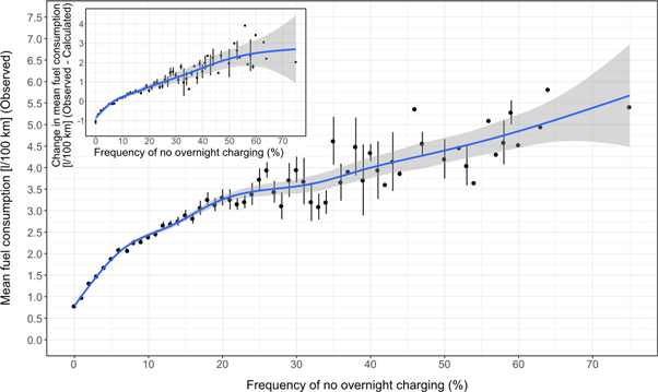
Figure 1. Mean fuel consumption versus frequency of no overnight charging, change in mean fuel consumption (observed-calculated) versus frequency of no overnight charging given inset.
Download figure:
Standard image High-resolution imageGiven inset in figure 1, we control for daily VKT and look at the isolated effect of no overnight charging. This is done by looking at the difference between observed mean fuel consumption and calculated mean fuel consumption, where the calculated mean fuel consumption refers to 1- UFcal multiplied by the fuel consumption in charge sustaining mode. From the inset in figure 1, we observe that regularly charging once overnight can result in a reduced observed mean fuel consumption of 1 litres per 100 km compared to a calculated mean fuel consumption, whereas not charging overnight 70% of the time can increase the observed mean fuel consumption by 3 litres per 100 km.
In figure 1, we observe that mean fuel consumption tends to increase in a steeper slope below 10% frequency of no overnight charging. We observe a different trend from 10% frequency of no overnight charging to 20% where the slope is less steep, and another trend with even a less steep slope when the frequency of no overnight charging is above 20%. We have run a piecewise linear regression for these three different trends and we find that the frequency of no overnight charging is statistically significant at the 0.1% level for all three trends. Here we provide the estimates and the standard error as added uncertainty (±): we find that fuel consumption and tail-pipe emissions increase by 1.85 ± 0.03 l/100 km or 42.7 ± 0.8 gCO2 km−1 tail-pipe emissions from 0% to 10% driving days without overnight charging (going from charging overnight everyday to only 9 out of 10 driving days). Around the mean frequency of no overnight charging (4.7%), mean fuel consumption is close to 2 litres per 100 km. We find that fuel consumption and tail-pipe emissions increase by 0.94 ± 0.12 l/100 km or 21.6 ± 2.87 g tail-pipe CO2 per km from 10% to 20% driving days without overnight charging. Above 20% driving days without overnight charging, fuel consumption and tail-pipe emissions increase by approximately 0.42 ± 0.05 l/100 km or 9.73 ± 1.25 g tail-pipe CO2 per km every 10% driving days without overnight charging.
The effect of regularly charging overnight on UF can be observed in figure 2. Looking at the difference between observed and calculated UF (main figure), we find that high shares of not charging overnight have a substantial effect on UF and not charging overnight 60% of the time can reduce the UF as much as 50 percentage points compared to the calculated UF that presumes charging every night.
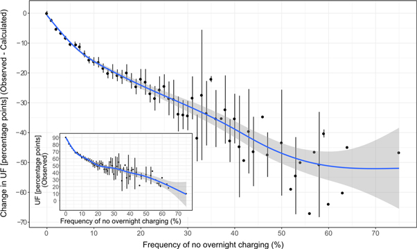
Figure 2. Change in UF (observed-calculated) versus frequency of no overnight charging, UF (observed) versus frequency of no overnight charging given inset.
Download figure:
Standard image High-resolution image3.3. Effect of charging more than once per driving day
From figure 3, we observe that the effect of an additional charging event is less substantial compared to overnight charging, yet higher shares of additional charging results in lower mean fuel consumption. In figure 3, we observe that the mean fuel consumption is level around 1.6 l/100 km or 37 g tail-pipe CO2 per km below 20% driving days with additional charging. A piecewise linear regression reveals that there is no statistically significant relationship between additional charging and fuel consumption when additional charging frequency is below 20%. Above 20% driving days with additional charging, regression analysis reveals a statistically significant relationship at the 0.1% level between additional charging and fuel consumption; and mean fuel consumption and tail pipe emissions decrease, on average by 0.08 ± 0.02 l/100 km or 1.86 ± 0.46 gCO2 km−1 tail-pipe CO2 per km every 10% driving days with additional charging.
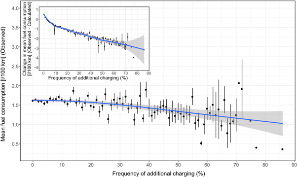
Figure 3. Mean fuel consumption (observed) versus frequency of additional charging, change in mean fuel consumption (observed-calculated) versus frequency of additional charging given inset.
Download figure:
Standard image High-resolution imageGiven inset in figure 3, if we control for daily VKT and look at the isolated effect of additional charging, we observe more clearly that an increase from 0% to 10% driving days with additional charging can result in a reduced observed mean fuel consumption of approximately 1 ¼ l/100 km or 29 g tail-pipe CO2 per km. Above 10% driving days with additional charging, we find a reduced observed mean fuel consumption of approximately 0.3 l/100 km or 6.9 g tail-pipe CO2 per km every 10% driving days with additional charging; e.g. 80% of driving days with additional charging can reduce observed mean fuel consumption by 3 l/100 km or 69 g tail-pipe CO2 per km.
The effect of additional charging on UF can be observed in figure 4. Frequency of additional charging, as given in the inset of figure 4, has a smaller effect on observed UF compared to no overnight charging. However, if we control for daily VKT and look at the difference between observed UF and calculated UF, we see that additional charging around 80% of the time has the potential to increase the observed UF around 50 percentage points compared to the calculated UF.
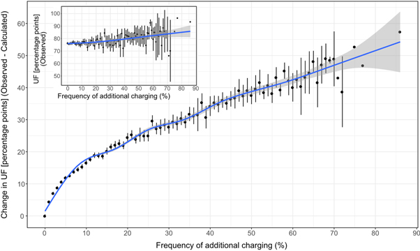
Figure 4. Change in UF (observed-calculated) versus frequency of additional charging, UF (observed) versus frequency of additional charging given inset.
Download figure:
Standard image High-resolution image3.4. Regression analysis
We use a multivariable regression analysis for a quantitative assessment of the effect of charging on fuel consumption. We distinguish between the frequencies of additional charging and the frequency of no overnight charging. Furthermore, we control for two additional variables with noteworthy impact on the UF and fuel consumption: the user's average daily VKT and the standard deviation (SD) of the daily VKT. The former indicates the typical daily driving distance while the latter also captures the variation in daily VKT where high SD is indicative of more frequent long-distance driving which additionally lowers the UF and increases fuel consumption at fixed mean daily VKT (Plötz et al 2018).
Our regression model is the following:

Where  denotes fuel consumption in litres per 100 km, fadditional charging is the frequency of additional charging (in %), fno charging is the frequency of no overnight charging (in %) and the last two variables denote the mean and SD of daily VKT (both measured in km). We use the log of the charging frequencies as this reduces the likelihood of heteroscedasticity. See the appendix for the detailed discussion and robustness checks on heteroscedasticity and normality assumption in our model. The inclusion of the mean and SD of daily VKT reduces potential omitted variable bias.
The results of the regression analysis are given in table 2. Note that the number of users in the regression analysis is slightly less than what is presented in table 1 due to omission of users with 0% frequency of no overnight charging or additional charging.
Table 2. Regression results for dependent variable fuel consumption. Shown are coefficient estimates with standard errors in parentheses.
| Dependent variable | Fuel consumption (l/100 km) |
|---|---|
| Intercept | 1.79*** (0.06) |
| (Log of) frequency of no overnight charging | 0.42*** (0.01) |
| (Log of) frequency of additional charging | −0.05*** (0.01) |
| Mean daily VKT | 0.0009* (0.0004) |
| SD of mean daily VKT | 0.01*** (0.0003) |
| Sample Size N | 6245 |
| Multiple R-squared | 0.669 |
| Adjusted R-squared | 0.669 |
| F-statistic | 3158 (p-value: < 0.0001) |
Confidence levels: *** %99.9, **%99, *%95
The model itself and all variables are significant (mean daily VKT at 5% level and all others at 0.1% level) and have the expected sign. The simple model explains about 67% of the variance in fuel consumption, which is acceptable for the low number of variables included. An increase in no overnight charging, i.e. a decrease in charging leads to higher fuel consumption. Likewise, an increase in additional charging reduces fuel consumption and increases the UF. Higher mean daily VKT leads to a higher fuel consumption as a fewer share of km is driven on electricity. Finally, a higher SD of daily VKT indicates more frequent long-distance driving and thus lower UF coupled to higher fuel consumption.
We observe that both the log of frequency of no overnight charging and additional charging are statistically significant. For every relative 10% increase in the frequency of no overnight charging (e.g. from 10% to 11%), fuel consumption increases by 0.017 l/100 km (calculated by log(1.1)*0.42) and tail-pipe emissions increase by 0.40 gCO2 km−1. For every relative doubling of the frequency of no overnight charging (e.g. from 10% to 20%), fuel consumption increases by 0.13 l/100 km (calculated by log(2)*0.42) and tail-pipe emissions increase by 2.92 gCO2 km−1. On the other hand, for every relative 10% increase in the frequency of additional charging, (e.g. from 10% to 11%), fuel consumption decreases by 0.002 l/100 km and tail-pipe emissions decrease by 0.05 gCO2 km−1. Similarly, for every relative doubling of the frequency of additional charging, fuel consumption decreases by 0.015 l/100 km and tail-pipe emissions by 0.35 gCO2 km−1. For a concrete comparison, any relative doubling of the frequency of no overnight charging, for instance going from charging overnight 9 out of 10 nights (10%) to 8 out of 10 nights (20%) has almost ten times more impact on fuel consumption and tail-pipe emissions compared to a relative doubling in additional charging freqeuncy, for instance going from additional charging 4 out of 10 driving days to 8 out of 10 driving days. The regression analysis further establishes in a statistically significant way that no overnight charging has more impact on fuel consumption and tail-pipe emissions compared to additional charging.
Checking for multicollineratiy, the variance inflation factors for all variables in the regression model were low and less than 2.2. We tested the regression model with different treshold choices for the calculation of no overnight charging and additional charging frequencies. For the occurrence of additional charging, our assumption was that observed UF for a vehicle for that given day was at least 1.5 times higher than the calculated UF; we also tested for a threshold of 1.3 and 1.7. Similarly, for the occurrence of no overnight charging, our assumption was that observed UF is smaller than half (0.5) the calculated UF; we also tested for a threshold of 0.3 and 0.7. We only varied one threshold at a time, keeping the other same as in our base assumption. All cases of varying the threshold resulted in the same statistical significance for all variables and only slight differences in the estimation of the coefficients. We also tested the regression without the additional controls of mean and standard deviation of daily VKT and using the actual values for no overnight charging and additional charging frequency instead of the log of those frequencies. The results of these robustness checks on the regression analysis, including varying the thresholds, are given in table A1 in the appendix. We observe that the effect of frequency of no overnight charging is robust and significant in all cases, however the effect of frequency of additional charging is small and coefficient sign not robust without additional controls included in the regression. This is in line with our findings in sections 3.2 and 3.3. where we observe the significantly large impact of overnight charging on fuel consumption in figure 1, and that fuel consumption starts to decrease only after 20% of driving days with additional charging in figure 3. In our regression model, users with more than 20% additional charging frequency makes up approximately 14% of total users (886 users out of 6245). This shows that having high shares of days with additional charging (having more than 20% additional charging frequency) is limited to only a small percentage of all users and is not a common behavior; thus for the majority of users, additional charging has little impact on fuel consumption due to its low frequency.
4. Discussion
Our analysis is based on a large sample with a long observation period making it unique. While being ample in time and number it only covers one PHEV model with longer range and a low power internal combustion engine. This can partly explain the high UF in our sample compared to other samples as low system power correlates with higher UF, see e.g. (Plötz et al 2020b). A shorter range might e.g. reduce the propensity for charging (Tal et al 2014a, 2014b). It is possible that our high UF creates an upperbound limit on the effect of additional charging given that the starting fuel consumption is already pretty low (1.6 l/100 km).
The vehicles are driven mainly by private users who are likely to be early adopters. Still, average annual driving distance in our sample is similar to the average in the US (21,562 km annual driving distance for our sample compared to 21,700 km US average) (FHWA 2020) implying that the overall driving distances are not that different. Home charging availability may also be affected by the fact that the users are from North America. Other countries, such as Japan and the Netherlands might have very different charging conditions (Funke et al 2019). Our sample contains a very large number of users. Yet, the specific authentification and connection to the OnStar system requires some technical knowledge that could lead to some sampling bias. However, taking into account that early PHEV adopters are generally interested in new technologies and well-educated (Plötz et al 2014), any potential samplnig bias via Voltstats as source should be limited. Furthermore, our results are likely unbiased with respect to some months that Voltstats.net was running without the partnership of OnStar as the partnership with OnStar came shortly after the site was established and the site had relatively low users at that point (∼1000 users compared to the ∼7,500 users we have in our dataset).
One limitation of the extracted raw data from the website is the missing model year. The extracted raw data does not have the serial number information, with which the users register themselves within the groups, therefore making it impossible to check the connection between the user and the model year group. However, we compared the indication in some of the sites user groups about the vehicle model year to the first trip. Generally, the year of the first trip provides a useful indication to the model year but there are cases where the first trip happens in a year much later than the model year. Accordingly, the year of the first trip in the data is a good proxy for the model year and has thus been used but is not always correct.
Even given the limitations mentioned above, the observed change in UF in our study by less charging overnight is consistent with simulations for overnight charging for German passenger cars in Plötz et al (2020b). To some extent, low UF can be due to long-distance travel without a charging option at the start point. Yet, we control for the effect of daily km travelled by studying both the UF as observed and by comparing the actual UF to the calculated UF if the vehicle had fully recharged before departure (e.g. inset in figure 2). In both cases, the impact of additional charging or no charging on fuel consumption and UF are highly similar. We see this as a strong indication that the actual change in fuel consumption is from differences in charging behaviour and not from differences in daily km travelled.
In this paper, we choose to focus only on tail-pipe emissions and do not include in our analysis emisssions from the grid that might also vary depending on charging time.While the overall emissions of the PHEV are important, we find that less attention has been given to the tail-pipe emission and fuel consumption of PHEVs. These are important not only for climate mitigation purposes but also because fuel consumption has an affect on local air quality as well and is more directly affected by user behaviour.
We base our analysis on an estimate of charging events and not actual charging behavior. The merit of this is that our method can be used for a wider range of data sets since daily eVKT and daily driving distance is much easier to access than the actual charging behaviour. This however implies that we might have missed some charging events, e.g. additional charging events during the day if the daily eVKT was below the range. Still, such uncaptured charging events would have further lessened the impact of additional charging on the overall fuel consumption and thus would not change our results.
A potential extension of the present work could include the effect of auxilliaries such as heating and AC. This could be done by adding ambient temperature to the regression model shown above based on the registered location of the vehicle. However, this would require at least the daily mean temperature for every location and every driving date in the sample (several million driving days in several thousand locations). This data is not readily available and such an inclusion is beyond the scope of the present paper. Yet, Plötz et al (2020b) estimated the effect of mean ambient temperature on UF and find the UF is reduced by about 1 percentage point per degree Celsius below 10 °C. Adding ambient temperature to our analysis would be interesting but is not likely to have a large effect on our findings as temperature can be expected to be uncorrelated with daily driving distances and the availability of home or workplace charging. Thus, our results are likely unbiased with respect to outside temperature although temperature alone clearly has an effect on UF.
5. Conclusions
Using data from 7,491 Chevrolet Volts with a total 3.4 million driving days in the US and Canada we quantify the effect of daily charging on the utility factor, fuel consumption and consequently tail-pipe CO2 emissions. We find that overnight charging (or charging the battery fully once per day) is important for the environmental performance of PHEVs. From 0% to 10% of nights without overnight charging (from charging overnight every day to 9 out of 10 driving days), fuel consumption can increase by 1.85 ± 0.03 l/100 km and tail-pipe emissions can increase by 42.7 ± 0.81 gCO2 km−1. For any relative doubling in the freqeuncy of no overnight charging, fuel consumption increases 0.13 l/100 km and tail-pipe emissions increase by 2.92 gCO2 km−1.
For users with an additional charging frequency of at least 20%, increasing the frequency with 10 percentage points can result in a reduction of fuel consumption of 0.08 ± 0.02 l/100 km and tail-pipe emissions of 1.86 ± 0.46 gCO2 km−1. Any relative doubling in the frequency of additional day charging decreases the fuel consumption by 0.015 l/100 km and tail-pipe emissions by 0.35 gCO2 km−1. The difference between the effect of not charging on one out of 10 nights and the effect of additional charging demonstrate the importance of daily charging.
Our results have several policy implications. First, charging can reduce fuel use and GHG emissions of PHEVs. Accordingly, a roll-out of charging infrastructure and strong incentives to charge as frequently as possible can reduce PHEV emissions. Second, charging every day is most important and users without home charging option need particular attention as a few nights without charging clearly reduce the emissions benefit. This implies that home charging should be made widely available and easily possible, for example also in multi-family dwellings. Work place charging is the second most relevant option, as it is the second most frequent travel destination. Workplace charging would then serve as primary charging locations for users without home charging and as an important location for additional charging for users with home charging options. With regard to policy considerations, workplace charging could be exempted from fringe benefit taxation (i.e. the financial benefit for an employee to get free charging at the workplace should be exempted from income taxation) and the installation of workplace chargers incentivised. Third, incentives for PHEVs should be revised based on national monitoring of actual fuel consumption and tail-pipe emissions. Policy makers should be prepared to reduce these incentives if utility factors are low and there is evidence that PHEVs are not being regularly charged. Specific user groups, e.g. those lacking home charging, might need special consideration either by providing better charging opportunities or through limited incentives.
Acknowledgments
AM and FS acknowledge the funding of Swedish Electromobility Centre for this publication. PP acknowledges that this publication was written in the framework of the Profilregion Mobilitätssysteme Karlsruhe, which is funded by the Ministry of Economic Affairs, Labour and Housing in Baden-Württemberg and as a national High Performance Center by the Fraunhofer-Gesellschaft. Furthermore, PP acknowledges support from the Paris Reinforce EU Horizon 2020 project (grant agreement No 820846).
Data availability statement
The data generated and/or analysed during the current study are not publicly available for legal/ethical reasons but are available from the corresponding author on reasonable request.
Appendix
Appendix. A1. Robustness checks on the regression analysis
In table A1, we provide the results of the robustness checks we performed on the regression analysis. Notice that the sample size varies under different assumptions regarding the threshold for the occurrence of charging events. This is due to the slight change in number of users with 0% frequency of no overnight charging or additional charging under each assumption, which are omitted from the regression analysis.
Table A1. Regression results for dependent variable fuel consumption under different assumptions. Shown are coefficient estimates with standard errors in parentheses. VIF stand for variance inflation factor.
| Dependent variable | Fuel consumption (l/100 km) | VIF | |
|---|---|---|---|
| Base model | Intercept | 1.79*** (0.06) | — |
| (Log of) frequency of no overnight charging | 0.42*** (0.01) | 1.27 | |
| (Log of) frequency of additional charging | −0.05*** (0.01) | 1.53 | |
| Mean daily VKT | 0.0009* (0.0004) | 2.17 | |
| SD of mean daily VKT | 0.01*** (0.0003) | 1.65 | |
| Sample Size N | 6245 | ||
| Multiple R-squared | 0.669 | ||
| Adjusted R-squared | 0.669 | ||
| F-statistic | 3158 (p-value: < 0.0001) | ||
| Lowering the additional charging occurrence threshold (UFobs/UFcal > 1.3) | Intercept | 1.80***(0.05) | — |
| (Log of) frequency of no overnight charging | 0.42***(0.01) | 1.29 | |
| (Log of) frequency of additional charging | −0.06***(0.01) | 1.62 | |
| Mean daily VKT | 0.001**(0.0004) | 2.27 | |
| SD of mean daily VKT | 0.01***(0.0003) | 1.66 | |
| Sample Size N | 6645 | ||
| Multiple R-squared | 0.669 | ||
| Adjusted R-squared | 0.669 | ||
| F-statistic | 3362 (p-value: < 0.0001) | ||
| Increasing the additional charging occurrence threshold (UFobs/UFcal > 1.7) | Intercept | 1.78***(0.06) | — |
| (Log of) frequency of no overnight charging | 0.42***(0.01) | 1.27 | |
| (Log of) frequency of additional charging | −0.05***(0.01) | 1.49 | |
| Mean daily VKT | 0.001*(0.0004) | 2.11 | |
| SD of mean daily VKT | 0.01***(0.0003) | 1.63 | |
| Sample Size N | 5624 | ||
| Multiple R-squared | 0.665 | ||
| Adjusted R-squared | 0.665 | ||
| F-statistic | 2792 (p-value: < 0.0001) | ||
| Lowering the no overnight charging occurrence threshold (UFobs/UFcal < 0.3) | Intercept | 1.50***(0.06) | — |
| (Log of) frequency of no overnight charging | 0.36***(0.01) | 1.19 | |
| (Log of) frequency of additional charging | −0.09***(0.01) | 1.45 | |
| Mean daily VKT | 0.003***(0.0004) | 2.10 | |
| SD of mean daily VKT | 0.01***(0.0003) | 1.66 | |
| Sample Size N | 5864 | ||
| Multiple R-squared | 0.637 | ||
| Adjusted R-squared | 0.637 | ||
| F-statistic | 2577 (p-value: < 0.0001) | ||
| Increasing the no overnight charging occurrence threshold (UFobs/UFcal < 0.7) | Intercept | 1.78***(0.05) | — |
| (Log of) frequency of no overnight charging | 0.46***(0.01) | 1.32 | |
| (Log of) frequency of additional charging | −0.03***(0.01) | 1.60 | |
| Mean daily VKT | 0.0008*(0.0003) | 2.25 | |
| SD of mean daily VKT | 0.01***(0.0003) | 1.62 | |
| Sample Size N | 6487 | ||
| Multiple R-squared | 0.687 | ||
| Adjusted R-squared | 0.687 | ||
| F-statistic | 3566 (p-value: < 0.0001) | ||
| Using actual values for the frequencies of no overnight charging and additional charging instead of using log of those frequencies | Intercept | 0.07***(0.02) | — |
| Frequency of no overnight charging (0 to 1) | 7.48***(0.14) | 1.22 | |
| Frequency of additional charging (0 to 1) | −1.04***(0.07) | 1.61 | |
| Mean daily VKT | 0.002***(0.0004) | 2.32 | |
| SD of mean daily VKT | 0.01***(0.0003) | 1.62 | |
| Sample Size N | 6245 | ||
| Multiple R-squared | 0.680 | ||
| Adjusted R-squared | 0.680 | ||
| F-statistic | 3317 (p-value: < 0.0001) | ||
| Excluding additional controls of mean and standard deviation of daily VKT | Intercept | 4.01***(0.04) | — |
| (Log of) frequency of no overnight charging | 0.62***(0.01) | 1.01 | |
| (Log of) frequency of additional charging | 0.04***(0.01) | 1.01 | |
| Sample Size N | 6245 | ||
| Multiple R-squared | 0.436 | ||
| Adjusted R-squared | 0.436 | ||
| F-statistic | 2411 (p-value: < 0.0001) |
Confidence levels: *** %99.9, **%99, *%95
In table A2, we provide the robustness checks on heteroscedasticity. Our regression model uses the ordinary least squares (OLS) method which assumes that the error terms all have the same variance (homoscedasticity). We ran the Breusch–Pagan test to check for heteroscedasticity. Using the log of frequency variables reduces the Breush-Pagan test statistic from 523.9 to 349.2; however, the p-value is still less than 0.0001 which suggests that our model has heteroscedasticity. This shows that using the log of dependent variables reduces the likelihood of heteroscedasticity and makes our model more appropriate for OLS but it does not remove it completely. To estimate the severity of heteroscedasticity and whether it has a significant impact on our estimates and the significance of those estimates, we applied appropriate methods to deal with heteroscedasticity and compared it to our base model. The two most common ways to deal with heteroscedasticity is (1) to use heteroscedasticity-consistent standard errors and (2) to use the weighted least squares method (WLS). We provide the regressions results with both of these methods in table A2. Using heteroscedasticity-consistent standard errors does not change the coefficient estimates but aims to improve the standard errors by addressing the problem of errors not being independent and identically distributed. As shown in table A2, using heteroscedasticity-consistent standard errors produce the same result as our base model. Standard errors are slightly improved only in the 6th and 7th decimal places, which is not shown in the table due to rounding. All dependent variables also have the same level of significance. When we use the WLS method, we observe no visible changes in standard errors except for the intercept where it goes down from 0.06 to 0.05; there are slight improvements in the standard errors of our dependent variables but only in the 6th and 7th decimal places, therefore not visible in table A2. The coefficient estimates change slightly only for the intercept (from 1.79 to 1.60) and the log of frequency of no overnight charging (from 0.42 to 0.38). We also observe that the mean daily VKT loses its significance. Multiple and adjusted R-squared values are lower compared to our base model (from 0.669 to 0.650). Overall, WLS method does not provide any significant improvements, and it ends up resulting in a lower multiple and adjusted R-squared. In conclusion, these two methods (heteroscedasticity-consistent standard errors and WLS) provide no significant improvements on our model. This shows that the heteroscedasticity in our model is not severe and does not affect our coefficient estimates and standard errors in any significant way. Therefore, we kept our base model with OLS estimators.
Table A2. Regression results for dependent variable fuel consumption using heteroscedasticity-consistent standard errors (robust standard errors) and weighted least squares (WLS) method. Shown are coefficient estimates with standard errors in parentheses.
| Dependent variable | Fuel consumption (l/100 km) | |
|---|---|---|
| Heteroscedasticity-consistent standard errors | Intercept | 1.79***(0.06) |
| (Log of) frequency of no overnight charging | 0.42***(0.01) | |
| (Log of) frequency of additional charging | −0.05***(0.01) | |
| Mean daily VKT | 0.0009* (0.0004) | |
| SD of mean daily VKT | 0.01*** (0.0003) | |
| Sample Size N | 6245 | |
| Multiple R-squared | 0.669 | |
| Adjusted R-squared | 0.669 | |
| F-statistic | 2407 (p-value: < 0.0001) | |
| Weighted least squares (WLS) | Intercept | 1.60***(0.05) |
| (Log of) frequency of no overnight charging | 0.38***(0.01) | |
| (Log of) frequency of additional charging | −0.05***(0.01) | |
| Mean daily VKT | 0.0004 (0.0004) | |
| SD of mean daily VKT | 0.01***(0.0003) | |
| Sample Size N | 6245 | |
| Multiple R-squared | 0.650 | |
| Adjusted R-squared | 0.650 | |
| F-statistic | 2898 |
Confidence levels: *** %99.9, **%99, *%95
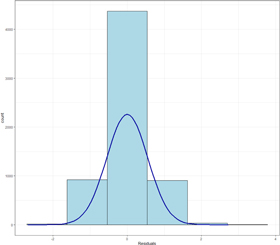
We also test the normality assumption in OLS which assumes that the residuals are normally distributed. It should be noted that with larger sample sizes, the assumption of normality becomes less essential. This is due to Central Limit Theorem (CLT) which assures that the sampling distribution of the estimates will converge toward a normal distribution as N increases (Pek et al 2018). Statistical tests that are used to check for the normality assumption, such as the Anderson-Darling test and Shapiro-Wilks test, also become more difficult to interpret as the sample size increases. With large sample sizes, the power of the test increases such that it can find non-normal distributions with very small deviations. Given our large sample size, we used the graphical method of residual histogram and then checked for two statistical measures of shape, skewness and kurtosis to test for normality. The residual distribution of our regression model has a skewness of 0.29 and a kurtosis of 3.98. A skewness between −0.5 and 0.5 suggests that the distribution is approximately symmetric. Kurtosis for a normal distribution is 3; therefore, a kurtosis of 3.98 suggests that our residual distribution has a slightly higher central peak. The residual histogram is given below in figure 5. We observe no violation of the normality assumption.
Figure 5. Histogram of residuals of the regression model.
Download figure:
Standard image High-resolution image