

Abstract
Around the Persian (Arabian) Gulf, a considerable volume of freshwater is obtained by desalination of seawater with the residual brine dumped back into the Gulf. This discharge of saltier waters impacts the marine ecosystem and may also affect dynamic and thermodynamic processes. Here, a fully non-linear, high-resolution numerical model is used to investigate the physical impacts of brine discharge into the Gulf. Twin runs were executed. One with and another without brine discharge at specific points. The results show that, when brine is injected, surface gravity waves irradiate from the locations and induce perturbations in other thermodynamic variables in the far field. Instead of attenuating, the anomalies have long term impact. The differences between the two experiments show marked seasonal and spatial variability. The largest differences occur during the summer and are located mainly along the axis of the Gulf's deeper channel. After 5 years of run, a budget calculation shows basin wide saline increase of about 0.2 g/kg, in agreement with previous studies. This might appear small when compared with the present Gulf mean salinity. However, the small change seems to be associated with significant variability in the spatial distribution and in the seasonal variability at different locations. It is found that there are regions in the Gulf where the standard deviation may represent serious consequences for living organisms in the marine environment.
Export citation and abstract BibTeX RIS

Original content from this work may be used under the terms of the Creative Commons Attribution 4.0 licence. Any further distribution of this work must maintain attribution to the author(s) and the title of the work, journal citation and DOI.
1. Introduction
The discovery of large oil fields in the Arabian Peninsula and other countries in the Middle East has resulted in the fast growth of the human population in the area. This has severely augmented the effects of the already existing and chronic shortage of potable water in the region, particularly in the arid Arabian Peninsula, where annual average rainfall lies in between 50 and 100 mm and the average evaporation rate can be higher than 3000 mm per year [e.g.:] (Al-Mutaz 2000, Paleologos et al 2018, Ibrahim and Eltahir 2019). Presently, the Middle East and North Africa (MENA) countries account for approximately 6% of the world's population but have less than 2% of the world's renewable freshwater supply. At the same time, the per capita water consumption, especially in the countries surrounding the Persian (or Arabian) Gulf (hereinafter referred simply as the Gulf), is among the highest in the world.
Surface water resources in the Arabian Peninsula are scarce and, despite the existence of underground aquifers, these are generally fossil deposits, not adequately recharged due to the low precipitation. In addition, a large fraction of the underground water supply has high salt content, requiring desalinization for agricultural purposes and other human-related consumption (Al-Mutaz 2000). Recent discovery of 'mega aquifers' [e.g.:] (Morton 2019), show the existence of some renewable underground water deposits in the Arabian Peninsula. Nevertheless, with the ongoing increased demand, the available water supply is expected to be halved by 2050 according to reports of the World Bank (WorldBank 2017). Pressured by the shortage and the increasing need for potable water, many countries in the region have resorted to desalination plants, in which freshwater is obtained from seawater or saline waters from underground deposits. The Gulf countries: Saudi Arabia, the United Arab Emirates (UAE), Kuwait, Qatar, Bahrain, Iraq and Iran, account for nearly two-thirds of the worldwide production of desalinated water (Al-Mutaz 2000, Lattemann and Höpner 2008, Ibrahim and Eltahir 2019, Paleologos et al 2018). Table 1 shows that, from a list of the top 20 desalination plants in the world, 12 are located around the Gulf.
Table 1. Worldwide top ranked desalination plants. Twelve of them are located around the Gulf. The numbers may not reflect the actual freshwater production because as of 2019 some of the plants were still being updated to the full desigened capacity—Data adopted from http://worldwater.org/wp-content/uploads/2013/07/table21.pdf and https://www.aquatechtrade.com/news/desalination/worlds-largest-desalination-plants/.
| Rank | Desalination Plant | Country | Gulf | LON | LAT | Designed Capacity |
|---|---|---|---|---|---|---|
| # | m3/day | |||||
| 1 | Ras Al Khair | KAS | Yes | 49.17°E | 27.50°N | 1,401,000 |
| 2 | Al Taweelah | UAE | Yes | 54.69°E | 24.75°N | 909,200 |
| 3 | Shuaiba 3 | KAS | 39.56°E | 20.63°N | 880,000 | |
| 4 | Ras Al Zour | KAS | Yes | 49.14°E | 27.54°N | 800,000 |
| 5 | Sorek | Israel | 34.73°E | 31.94°N | 624,000 | |
| 6 | Rabigh 3 | KAS | 39.00°E | 22.75°N | 600,000 | |
| 7 | Jebel Ali M | UAE | Yes | 55.12°E | 25.06°N | 600,000 |
| 8 | Fujairah | UAE | 56.37°E | 25.31°N | 591,000 | |
| 9 | Al Zour North | Kuwait | Yes | 48.38°E | 28.71°N | 567,000 |
| 10 | Shweihat | UAE | Yes | 52.57°E | 24.15°N | 455,000 |
| 11 | Shweihat 2 | UAE | Yes | 52.57°E | 24.15°N | 454,600 |
| 12 | CA San Francisco | USA | 122.38°W | 37.75°N | 454,200 | |
| 13 | Qidfa | UAE | 56.37°E | 25.29°N | 454,000 | |
| 14 | Al Jubail | KAS | Yes | 49.61°E | 27.05°N | 408,600 |
| 15 | Ashkelon | Israel | 34.53°E | 31.64°N | 395,000 | |
| 16 | Jebel Ali L-2 | UAE | Yes | 55.12°E | 25.07°N | 363,200 |
| 17 | TX Pt. Comfort | USA | 96.55°W | 28.65°N | 340,650 | |
| 18 | Jebel Ali L-1 | UAE | Yes | 55.12°E | 25.06°N | 317,800 |
| 19 | Jebel Ali N | UAE | Yes | 55.12°E | 25.06°N | 300,000 |
| 20 | Sulaibya | Kuwait | Yes | 4779°E | 29.38°N | 300,000 |
In a desalination plant, the byproduct from the freshwater extraction is a brine with higher concentration of salt and other elements. In the desalination process, a large number of different elements such as chlorine, copper sulfate, sodium bisulfate, ferric chloride, sulfuric acid, etc are added either before after the water filtration (Al-Mutaz 2000, Lattemann and Höpner 2008, Paleologos et al 2018, Ibrahim and Eltahir 2019). The resulting brine is then discharged into the surrounding bodies of water. Although not entirely understood, it is unquestionable that the injection of salt and other contaminants may have serious impacts on chemical, biological, and physical processes. A large number of studies have been published on the technical aspects of the desalination process, the disposal methods, the regulations and the impacts of brine on the physics and biogeochemistry of the marine environment [e.g.:] (Al-Mutaz 2000, Smith et al 2007, Dawoud and Mulla 2012, Ahmad and Baddour 2014, Joydas et al 2015, Lattemann and Höpner 2008, Paleologos et al 2018, Lee and Kaihatu 2018, Ibrahim and Eltahir 2019, Frank et al 2019, Petersen et al 2019, Wood et al 2020). Fewer studies, however, are based on high-resolution numerical models to investigate the interplay between the brine and the larger-scales ambient currents (Baum et al 2018, Perez-Diaz et al 2019, Chow et al 2019 , Ibrahim and Eltahir 2019).
From the total of over 10 million cubic meters extracted daily by the plants listed in table 1, a combined volume of 6,876,400 m3 (approximately 63%) of freshwater is processed each day by the plants around the Gulf. Assuming that the entire volume is extracted from and the resulting brine returned to the Gulf, and considering a mean salinity of 40 psu (one psu is equivalent to one part per thousand or ppt), a quick back-of-the-envelope calculation yields a volume of 2.75 × 10⁵ m3 of salt injected daily into the Gulf. In a closed domain, the net removal of freshwater would ultimately lead to a volume decrease and an increase in salt concentration (salinity). In reality, however, the Gulf is not an enclosed sea. It exchanges water via the Strait of Hormuz with the Indian Ocean. To compensate the net loss of water due to excess evaporation (and anthropogenic freshwater extraction), there must be an inflow of fresher waters from the Arabian Sea in the upper layers and the export of saltier waters near the bottom. This inverse estuary-like circulation setup results in the net import of approximately 0.2 million cubic meters per second of freshwater-equivalent into the Gulf.—as explained in (Campos et al 2020, Johns et al 2003), 'freshwater equivalent' is the opposite of the total flux of salt divided by a reference salinity—However, in spite of the freshening effects of this exchange of waters with the Indian Ocean, this is not a linear and straightforward process. Small changes in the water density can lead to unpredictable changes in the circulation and on the freshwater budget.
Using a high-resolution coupled ocean-atmosphere model with a 3D unstructured grid hydrodynamic component, Ibrahim and Eltahir (2019) simulated the dynamic interplay between brine discharge and Gulf residual circulation. By comparing the results of experiments without and with brine discharge from the 24 largest-capacity plants inside the Gulf, totaling approximately 11 million cubic meters of freshwater per day), they found an overall salinity increase in the Gulf of about 0.43 g/kg.—In spite of the different units for salinity adopted in different publications (g/kg, ppt, psu), they are practically equivalent and interchangeable for the purposes of the present work [e.g.:] (Lewis 1980)—Ibrahim and Eltahir (2019) concluded that, while the basin wide salinity is insensitive to brine discharge, the regional sensitivity is significant, especially in the southwestern regions near the Arabian coast. In a similar study using a numerical model (Lee and Kaihatu 2018), comparison between experiments with and without desalination in the Gulf showed, after 12 years of simulation, a basin wide increase in salinity of about 0.2 psu (ppt in the reference).
Here we apply a high-resolution, state-of-the-art ocean general circulation model (OGCM) to investigate the impact of the desalination on the mean state and variability of the physical environment, as a first step of a longer-term multidisciplinary investigation. Due to the lack of field data, the results of the numerical experiments are compared with those of the studies referenced in the previous paragraph (Ibrahim and Eltahir 2019, Lee and Kaihatu 2018). Two experiments were executed considering the same conditions except that in one of them a set of virtual desalination plants is considered. Folowing these introductory remarks, the remaining of the manuscript is structured as follows. In section 2, a brief but comprehensible description of the numerical model is given and the methodological approach used in the freshwater budget is described. The results are presented and discussed in section 3. Finally, section 4 summarizes the most relevant conclusions.
2. Materials and methods
2.1. The numerical model
The numerical simulations were run with a high-resolution (Δx = Δy = 1/36-degree or ≈2.8 km) implementation of the Hybrid Coordinate Ocean Model (HYCOM) (Bleck 2002, Halliwell 2014). The experiments considered the geographic domain delimited by latitudes 9.3°S–30.6°N and longitudes 33.0°E–76.9°E (figure 1). The vertical structure was discretized in 22 hybrid layers, all of them allowed to transform from isopycnic to terrain-following or to z-coordinates. The bathymetry was based on the NOAA-NGDC's ETOPO1 dataset (Amane and Eakins 2009). The shallowest depths were kept in 2 meters (regions with depths less than 2 meters were considered land). A one-way nesting scheme was used to provide the initial and boundary conditions. This approach, similar to the one used by (Campos et al 2020), is summarized as follows. First, a global 1/12-deg, 32-layers experiment with HYCOM was initialized with results downloaded from the HYCOM Consortium and forced for 21 years with products from the Comprehensive Ocean and Atmosphere Data Set (COADS) (Woodruff et al 1987). For lack of data storage space, a decision was made to save only the averages every six days of the global run products. Following, the available six-days averages of all relevant fields from the global run, starting on day 355 of the climatological year 21, were remapped onto the 22 isopycnic surfaces and interpolated to the 1/36-deg horizontal grid used in the present work. Then, the experiments with the nested model were executed using the interpolated global products as initial and boundary conditions, also forced with COADS climatological products. The COADS forcing fields used consisted of surface air temperature, net downward radiation flux, net downward shortwave flux, precipitation, vapor-mixing ratio, surface wind speed and wind stress. Similarly as in (Campos et al 2020), at each time step, the products of the model's integration were relaxed to the boundary conditions, in a 36 grid-points 'buffer' zone with an e-folding time of 53 days.
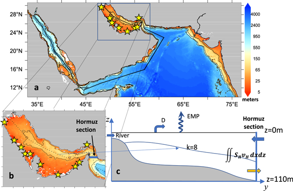
Figure 1. a: Bathymetry, from ETOPO1 (Amane and Eakins 2009), for the entire area in the numerical experiments. b: Zoom of the Gulf region considered for the analyses reported in the present papers. c: Schematics of the elements considered in the salt/freshwater flux budget. The line labeled k = 8 is the isopycnic surface σt = 27.70 kg m−3.
Download figure:
Standard image High-resolution imageA pair of twin-runs were performed for the entire oceanic region shown in the bottom panel (a) of figure 1, including the Arabian Sea, the Gulf and the Red Sea. In the first run, hereinafter referred as NODESAL, no anthropogenic salt input was considered. In the second, hereinafter referred as DESAL, selected desalination plants were included around the Gulf in the form of 'negative rivers' or 'rivers of salt', mainly along the Arabian Peninsula coastline. Both experiments included the most significant rivers in the modeled region. For more details on the rivers and desalination plants, see table 2. The climatological values for the riverine inflows (here, 'inflow/outflow' indicates water into/from the Gulf), in cubic meters per second (m3 s−1), were obtained from a global database of monthly mean river discharge constructed at the U.S. Naval Research Laboratory (Barron and Smedstad 2002). In the entire area considered in the model, nine rivers with mean flow larger 128m3s−1 were considered. From these, only three discharge their waters directly inside the Gulf: The Shatt-al-Arab, the Karun and Karkkeh. The combined mean inflow of these three rivers is 2,900m3 s−1 on average, according to table 2. At each of the desalination plants, due to the lack of more accurate information in the literature, the freshwater outflow was prescribed in a somewhat arbitrary way, in general, reflecting the order of magnitude of the values listed in table 1. The total mean value of the ten plants listed in table 2 is of 120 m3 s−1, which is higher than the total value of approximately 80 m3 s−1 from the Gulf's twelve plants listed in table 1. It is likely that the actual values are either higher than those disclosed by the plants or will be in a short while.
Table 2. Name, location and average volumes of riverine inflows and desalination plants outflows. The rivers indicated with the the dagger sign (†) are located inside the Gulf. While the river discharges are considered positive (inflows), the freshwater removed by the desalination plants are negative (outflows). The river data were taken from (Barron and Smedstad 2002).
| # | Name | Country | Location | Mean flow |
|---|---|---|---|---|
| (m3/s) | ||||
| R1 | Indus | Pakistan | 67.50°E, 24.00°N | 6,092 |
| R2 | Shatt-al-Arab† | Iraq | 49.00°E, 30.00°N | 2,280 |
| R3 | Narmada | India | 72.50°E, 21.50°N | 1,401 |
| R4 | Tapi | India | 72.60°E, 21.40°N | 469 |
| R5 | Karun† | Iran | 48.80°E, 30.00°N | 486 |
| R6 | Mahi | India | 72.50°E, 21.50°N | 382 |
| R7 | Periyar | India | 76.20°E, 10.20°N | 162 |
| R8 | Karkkeh† | Iran | 48.50°E, 30.00°N | 161 |
| R9 | Kalinadi | India | 74.10°E, 15.00°N | 128 |
| D1 | Hamryia | UAE | 55.47°E, 25.45°N | −15 |
| D2 | Jebel Ali | UAE | 55.10°E, 25.08°N | −20 |
| D3 | Mirfa | UAE | 53.42°E, 24.24°N | −15 |
| D4 | Al Khobar | KSA | 50.22°E, 26.18°N | −10 |
| D5 | Jubail | KSA | 49.78°E, 26.93°N | −10 |
| D6 | Kuwait | Kuwait | 48.00°E, 29.39°N | −10 |
| D7 | Iran | Iran | 56.10°E, 27.12°N | −10 |
| D8 | QEWC | Qatar | 51.63°E, 25.07°N | −10 |
| D9 | Ras Abu Fontas | Qatar | 51.63°E, 25.08°N | −10 |
| D10 | Ras Abu Jarjur | Barhrain | 50.63°E, 26.18°N | −10 |
In both experiments, tidal forcing was not considered in the simulations. Findings of previous studies show that, despite their relevance on the shorter term, tides do not generate significant residual currents in the longer time scales in the Gulf [e.g.:] (Pous et al 2012, 2015). However, this does not mean that residual currents resulting from non-linear interactions of the tidal flow with topography should be completely ignored. There are regions in the Gulf where the residual currents can exceed 0.15 m/s, or about 10% of the local barotropic velocity (Poul et al 2016). The effects of tides will be addressed in future experiments.
The products of a 6-years numerical integration, from Jan-01-0022 to Jan-01-0027, were saved daily, for both the internal (baroclinic) and external (barotropic) modes at each point of the entire grid.
2.2. Methodology to compute the freshwater trend
One of the objectives of the present work is to assess the significance of any salinity increase associated with the extraction of freshwater at locations along the Gulf's shores. For doing that, a methodology to calculate the salt budget and any resulting trend was devised considering a semi-enclosed sea as represented in top right panel (c) of figure 1. The equations for conservation of volume (V) and total salt content (S) within the region can be written as follows.

and

In these equations, Vt
= ∂V/∂t is the volume trend; St
= ∂S/∂t is the total salinity trend;  is the volume-averaged salinity; EMP is the evaporation minus precipitation over the Gulf and D is the total volume of water extracted by the desalination plants. SEMP represents the net flux of salt associated with evaporation minus precipitation and SD is the total salt influx resulting from the desalination process. RestV
and RestS
are residual terms due to small scale mixing and truncation errors, v is the meridional component of the velocity and the subscript H indicates the variable at a vertical section across the Strait of Hormuz (see figure 1). Note that volume trend term (Vt
) is the link between the two equations.
is the volume-averaged salinity; EMP is the evaporation minus precipitation over the Gulf and D is the total volume of water extracted by the desalination plants. SEMP represents the net flux of salt associated with evaporation minus precipitation and SD is the total salt influx resulting from the desalination process. RestV
and RestS
are residual terms due to small scale mixing and truncation errors, v is the meridional component of the velocity and the subscript H indicates the variable at a vertical section across the Strait of Hormuz (see figure 1). Note that volume trend term (Vt
) is the link between the two equations.
As it is more intuitive to deal with volumes of water being extracted from or discharged into the sea, the salt budget equation (equation (2)) is transformed into an equivalent-freshwater (hereinafter simply freshwater) budget equation, dividing it by a reference salinity S0:

where
With the insertion of Vt from equation (1) into equation (3), the total freshwater trend, Mt , can be estimated by the equation:

Here,
where E—P (Evaporation minus Precipitation) is an output of the numerical model;

N is the number of desalination plants considered and Di the volume processed by each plant;

SS is the surface salinity and

Note that SRiv = 0 because the salinity S at the river mouth is equal to zero.
It is important to note that the terms multiplied by  in the above equations represent the contributions to the trend from the changes in volume. Although small, Vt
is not necessarily equal to zero since there are changes in SSH. In addition, it is assumed that the smaller scale effects and truncation errors in the twin runs are equivalent (perhaps this is not entirely true but the differences between these terms are expected to by small enough to be neglected). Thus, the difference between the results of equation (4) for the two experiments (DESAL—NODESAL) eliminates the residual terms and yields an equation for computing
in the above equations represent the contributions to the trend from the changes in volume. Although small, Vt
is not necessarily equal to zero since there are changes in SSH. In addition, it is assumed that the smaller scale effects and truncation errors in the twin runs are equivalent (perhaps this is not entirely true but the differences between these terms are expected to by small enough to be neglected). Thus, the difference between the results of equation (4) for the two experiments (DESAL—NODESAL) eliminates the residual terms and yields an equation for computing  , the freshwater loss due to the desalination process within the modeled region:

3. Results and discussion
3.1. Simulations time-history
Each experiment was started on the 1st of January of climatological year 22 and let to run for five years, to 1st of January of year 27. The time-history of each realization is represented by the time series of the basin-averaged sea surface height (SSH) and kinetic energy (KE), plotted in figure 2. The plots show that it takes about one year for the model to reach a state of reasonable equilibrium in both experiments. After a pronounced spike in KE in the first year of the run, due to the initialization process, the curves show a more uniform behavior, with strong seasonality, certainly associated with the forcing seasonal variability. They also suggest some energy in higher and lower frequencies. The intraseasonal variability could be associated with either the forcing or nonlinear mesoscale features. However, since the model is forced with climatological products, with no year-to-year changes, the interannual variability displayed in the KE and SSH curves are certainly associated only with the model's internal variability. It is also relevant to point out that, despite being small, there are some noticeable differences between NODESAL and DESAL, especially in KE.
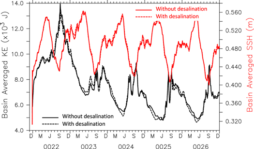
Figure 2. Time-history of the basin averaged SSH and KE for twin experiments.
Download figure:
Standard image High-resolution image3.2. The Gulf circulation according to the model
Because the main objective of this work is to investigate the differences between the two experiments, only a brief description of the model's general results is given here. As suggested by the KE and SSH curves in figure 2, in both experiments, with and without desalination, the circulation shows a marked seasonal variability. The spatial structure has a dominant two-layer structure, in good agreement with the general pattern described in the literature [e.g.:] (Reynolds 1993, Johns et al 2003, Campos et al 2020). Similarly to a previous work based on results of experiments with HYCOM (Campos et al 2020), in the upper-layer, defined by the model's top eight isopycnic surfaces, the horizontal circulation is dominated by a year-round cyclonic gyre, with less saline waters from the Gulf of Oman entering the Gulf through the Strait of Hormuz forming two branches. The northern branch flows along the Iranian coast, reaching the northwestern regions of the Gulf. The southern branch flows towards the coasts of the UAE and is the most affected by the seasonality, being stronger in the summer. In the winter, the top layer circulation has the two branches well defined but weaker mesoscale activity. Starting in April, strong meso-scale eddies start to form and remain until December, with a sequence of quasi-stationary cyclonic and anticyclonic vortices along the Gulf's deeper channel. In the bottom layer, the overall salinity is higher and the predominant direction of the flow is towards the Strait of Hormuz, in agreement with the inverse-estuary circulation patter described in previous works (Reynolds 1993, Johns et al 2003, Yao and Johns 2010, Campos et al 2020). This two-layer structure is well represented by the vertical structure of temperature, salinity and velocity on a section along 26°N, the 'Hormuz section', indicated in figure 1(b). As seen in figure 3, which represents the time averaged distributions, the velocity is positive (towards north) in the upper layer and negative (southward) in the bottom layer. The mean temperature decreases with depth while the salinity is lower in the region above the interface defined by the isopycnic layer k = 8 (σt = 24.70 kg m−3) and has higher values below. It should be pointed out that, despite the fact that the salinity distribution shows a region of lower salinity near the easter side of the vertical section, the density (panel c) increases monotonically with depth, indicating stability of the water column.

Figure 3. Mean vertical distributions of salinity (a), in g/kg; temperature (b), in °C; density anomaly (d), in kg m−3; and meridional velocity (d), in m s−1 at the 'Hormuz section', along 26°N (see figure 1). The light-blue curves over the density plot (c) are isohalines. The line labeled 'k = 8' is the isopycnic surface σt = 24.70 kg m−3, which delimits the upper and lower layers.
Download figure:
Standard image High-resolution image3.3. Impacts of brine discharge on the residual circulation
To assess the impact of the brine injection on the Gulf's residual circulation, differences between the two experiments (DESAL—NODESAL) for the seasonal means (Summer and Winter) and long term mean were taken. Figure 4 displays these differences for salinity (left panels) and velocity and SHH (right panels). In that figure, JAS and JFM seasons are, respectively, the averages for the months Jul-Aug-Sep and Jan-Feb-Mar of the last year of the run (Year 26). The 'Mean' is the time average for the period Jan-1-0023 to Jan-1-0027. In spite of the fact that the only difference between the two experiments was the extraction of freshwater in a few points, after five years there are relatively large differences in salinity, SSH and velocity, especially along the deeper channel of the Gulf, near the Iranian coast. These differences are prominent during JAS and appear closely related with the mesoscale activity that are more intense during the summer season.
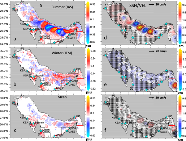
Figure 4. Differences between salinity, SSH and velocity from the two experiments (DESAL minus NODESAL), for JAS, JFM and long term mean.
Download figure:
Standard image High-resolution imageTo some extent, the large differences shown in figure 4 represent an intriguing result. To better understand these impacts of the brine injection (or freshwater extraction), an animated plot (figure S1 (available online at stacks.iop.org/ERC/2/125003/mmedia), Supplementary Material) was produced with a high-frequency sequence of snapshots of the difference in SSH (DESAL—NODESAL) during the first couple of days of run. The 'movie' shows that the perturbation of the sea level caused by the injection of salt at some points along the Gulf shores generates anomalies that propagate as surface gravity waves, reaching regions as far as the northern end of the Red Sea in less than 24 h. These SSH anomalies then generate disturbances in other properties, as in salinity, for instance, according to the physical process described as follows.
Consider the equation for conservation of salinity:

where KH and Kz are the horizontal and vertical components the turbulent diffusivity coefficient.
The integration of equation (6) from the bottom of an isopycnic layer (−h) to the sea surface (η) yields:

where Fη and F−h are, respectively, the salt fluxes across the free surface and the bottom of the layer.
The zonal and meridional components of the geostrophic velocity can be written as:


These two equations, equations (8) and (9), show that the geotrophic flow, the predominant component of the velocity in the meso-to-large scale dynamics, depends on the sea surface elevation η. On the other hand, the release of brine at a point changes the surface elevation, generating surface gravity waves that propagate with speed  . For instance, for H = 10 meters, c ≈ 10 m s−1 or 864 km/day. This means that SSH anomalies originating in the Gulf would propagate with speeds of about a thousand kilometers per day, or faster. Consequently, according to equation (7), other thermodynamic properties would be affected as well. Contrary to what one would expect, instead attenuating with time, the perturbations excite normal modes of variability, through some sort of resonance, or trigger mesoscale activities by means hydrodynamic instability. Although no further investigation was done to test these hypotheses, the fact is that, instead of dissipating, these small initial SSH anomalies ended up in the sustained and significant perturbations in the Gulf's salinity, SSH and velocity distributions shown in figure 4. The differences are much well pronounced during the summer months, July trough September (JAS), with relatively strong anomalies associated with the centers of cyclonic and anticyclonic circulation along the axis of the Gulf's deeper channel. During JAS, the salinity anomalies vary from near −0.60 to more than 0.60 psu. The range in SSH differences is from −10.0 to 10.0 cm while velocity can be as higher as 0.20 m s−1 over the deep channel. These differences are much weaker during the winter (JFM), especially in SSH and velocity. Although small, when compared with the values in JAS, the differences in the long-term means are not negligible.
The bottom left panel of figure 4 show that the difference (DESAL—NODESAL) in the mean surface salinity has a noticeable spatial variability. In particular, the areas surrounding Bahrain, Qatar and the northern coast of the UAE show more intense red colors than in other regions. This means that those areas may be more affected by the salt buildup resulting from the brine injection. To further investigate this possibility, the area averaged differences in the surface temperature and salinity distributions from the two experiments (DESAL—NODESAL) were plotted for six areas around of the desalination plants, as indicated in figure 5. For each of the areas labeled as Kuwait, KSA1/Bahrain, Qatar, UAE3, UAE1 and Iran, the 5-years mean and standard deviation were calculated, as listed in table 3. The results show that, in general, after five years of discharging brine in those specific areas, both mean changes of salt and temperature are very small. The highest values for the mean salinity, in the order of 0.1 psu are found in the KSA1/Bahrain and Qatar areas. Both of these locations show relatively small standard deviation. On the other hand, in the UAE1 region, in spite of the smaller mean salinity, in the order of 0.04 psu, the standard deviation is the highest, with a value of the order of 0.2 psu. In UAE1, there is also a relatively larger variability in the mean temperature, of about .016 °C as compared with the other sites, except for Kuwait. At this point one could argue that, considering that there is a constant input of salt, the mean values calculated for the entire period are not representative of the actual values at the end of the simulation. However, as clearly seen in the plots of figure 5, except for UAE1 and Iran, there are no noticeable trends in the time series. In the UAE1 area, considering only the last 24 months of the run, the mean temperature and salinity values are of the order of 0.2 °C and 0.2 psu, respectively. However, the plots for the UAE1 area also show considerable interannual variability. This raises a question on the statistical significance of the trend and suggests that the mean for only the last two years could be biased.
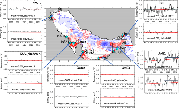
Figure 5. Time series of the differences (DESAL—NODESAL) in temperature and salinity averaged over areas around some desalination plants.
Download figure:
Standard image High-resolution imageTable 3. Mean and standard deviation for the area averaged differences (DESAL—NODESAL) in temperature and salinity in the vicinity of some desalination plants, as indicated in figure 5.
| Temp. (°C) | Saln. (psu) | |||
|---|---|---|---|---|
| Name | Mean | Stdv | Mean | Stdv |
| Kuwait | 0.021 | 0.033 | 0.040 | 0.017 |
| KSA1/Bahrain | 0.001 | 0.014 | 0.110 | 0.021 |
| Qatar | 0.003 | 0.010 | 0.075 | 0.017 |
| UAE3 | 0.000 | 0.004 | 0.048 | 0.010 |
| UAE1 | 0.016 | 0.154 | 0.043 | 0.198 |
| Iran | 0.011 | 0.101 | 0.027 | 0.039 |
3.4. Impacts on the equivalent-freshwater budget
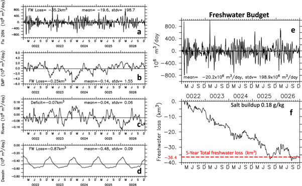
As mentioned in section 1, the Gulf is not an enclosed sea. By means of an inverse-estuary circulation, it exchanges water with the Indian Ocean and, to compensate the volume decrease due to the extraction of freshwater by the desalination process, water must be pumped in through the Strait of Hormuz. However, this is not a simple and straightforward dynamic process. The small changes due to brine injection into the Gulf lead to changes in the overall temperature and salinity, which lead to changes in EMP and in the residual circulation. The net result is that, in spite of maintaining the volume constant, the basin wide mean salinity would be different in unpredictable ways. To evaluate the changes resulting from the introduction of some desalination plants, as described in the previous sections, equation (5) was used to calculate the trend in the total volume of equivalent-freshwater in the Gulf. For that, the constant value of 39.64 psu was adopted for the reference salinity S0. The results are summarized in figure 6.
Figure 6. Results of the equivalent-freshwater budget calculations with equation (5). On the left panels (a)–(d) are plotted the terms in the RHS of equation (5). On the right (e) and (f) the plots represent the total freshwater trend ( ) and the accumulated loss in 5 years, respectively.
Download figure:
Standard image High-resolution image
On the left panels of figure 6, the individual terms on the right-hand-side of equation (5) are plotted: (a) the residual freshwater flux across 26°N; (b): the difference in EMP from the two experiments; (c): the net effect of the rivers discharge; and (d): the effect of brine injection. All values are in million cubic meters per day. On the right, the top panel (e) shows M*
t
, the sum of all RHS terms in equation (5), and in the lower panel (f) is the time integral of  , which represents the total freshwater loss due to the desalination process during the five years of the experiment. These results show that, when the changes associated with the volume trend (Vt
) are considered, the residual impacts of river inflow, EMP and the desalination plants outflow are relatively small, as compared with the lateral exchange at the Strait of Hormuz. The combined effect is a negative trend of 20.2 million cubic meters per day, resulting in a total loss of 36.4 km3 in five years. Considering the Gulf's mean volume of 8118 km3 (area of 2.39E+5 km2 and mean depth of 33.96m), this freshwater loss corresponds to a salinity increase of 0.18 psu in five years. This value is similar to the result obtained by (Lee and Kaihatu 2018), but only half of the salinity increase reported by (Ibrahim and Eltahir 2019). However, one must consider that the present study is based on only five years, as compared with the 12 years in the cited works (Lee and Kaihatu 2018, Ibrahim and Eltahir 2019).
, which represents the total freshwater loss due to the desalination process during the five years of the experiment. These results show that, when the changes associated with the volume trend (Vt
) are considered, the residual impacts of river inflow, EMP and the desalination plants outflow are relatively small, as compared with the lateral exchange at the Strait of Hormuz. The combined effect is a negative trend of 20.2 million cubic meters per day, resulting in a total loss of 36.4 km3 in five years. Considering the Gulf's mean volume of 8118 km3 (area of 2.39E+5 km2 and mean depth of 33.96m), this freshwater loss corresponds to a salinity increase of 0.18 psu in five years. This value is similar to the result obtained by (Lee and Kaihatu 2018), but only half of the salinity increase reported by (Ibrahim and Eltahir 2019). However, one must consider that the present study is based on only five years, as compared with the 12 years in the cited works (Lee and Kaihatu 2018, Ibrahim and Eltahir 2019).
4. Summary and conclusions
The desalination process extracts freshwater from seawater, returning to the marine environment a residual brine with high salt concentration. In Persian (Arabian) Gulf, where considerable volume of freshwater is obtained by desalination plants, it is ultimately important to understand the long-term environmental effects on the proccess. The discharge of brine into an oceanic region such as the Gulf has consequences not only for marine ecosystem, but can also affect the dynamic and thermodynamic processes. As a contribution to better understanding these non-linear impacts on the physical environment, a high-resolution numerical model was used to simulate the effects of injecting brine in some points along the Gulf's coastal region. Twins experiments were carried out, with the only difference that in one water was pumped out in some specific points. The results show that, at the very beginning, surface gravity waves propagate from these locations and result, in the long term, in significant changes in the basin wide distributions of temperature, salinity, SSH and velocity. The differences between the two experiments have marked seasonal and spatial variability, with the largest values occurring during the Summer (JAS) and located mainly along the Gulf's deeper channel. In five years after the start of the brine injection, the experiments show a basin wide salinity increase of about 0.2 psu. It is also found that, despite the overall small mean increase in salinity, there are regions where the standard deviation is considerably higher, which may represent serious consequences for the biological environment. These non-physical effects are being under investigation, as part of an ongoing effort in which the results of the present experiments will be used in combination with individual based models to study the impacts on coral reefs in the Gulf.
Acknowledgments
This work was funded by the American University of Sharjah (Grants FRG19-M-G67, FRG19-M-G74 and FRG20-M-S20). The numerical experiments were run in computer resources at the Laboratory for Ocean Modeling and Observations (LABMON), of the Oceanographic Institute of the University of São Paulo, Brazil, sponsored by the São Paulo State Foundation for Research Support (FAPESP, grant 2017/09659-6). All the data is freely available at https://doi.org/10.17882/77278. EC acknowledges the Brazilian Council for Scientific and Technological Development (CNPq) for a Research Fellowship (Grant 302 503/2019-6). This paper is Lamont–Doherty Earth Observatory contribution number 8458. The publication costs were fully covered by the Open Access Program from the American University of Sharjah (Grant OAP-CAS-052). This paper represents the opinions of the author(s) and does not mean to represent the position or opinions of the American University of Sharjah.