


Abstract
Flaring of natural gas contributes to climate change and wastes a potentially valuable energy resource. Various groups have estimated flaring volumes via remote sensing by nighttime detection of flares using multi-spectral imaging. However, only limited efforts have been made to independently assess the accuracy of these estimation methods. I analyze the accuracy of the VIIRS Nightfire published flare detection results, comparing yearly estimated flaring rates to reported flaring data from governments in 9 countries (Brazil, Canada, Denmark, Mexico, Netherlands, Nigeria, Norway, USA, UK) and 7 years (2012–2018 inclusive). We analyze only flares occurring at offshore oil and gas production platforms and floating production units. A total of 1054 flare volume estimates were compared to volumes reported to government agencies. 80.8% of flare estimates lie within 0.5 orders of magnitude (OM) of reported volumes, which 93.7% fall within 1 OM of the reported volume. Little systematic bias is found except in the smallest size classes (<106 m3 y−1). Relative error ratios are larger for smaller flares. No significant trend was observed across years, and variation by country is in line with that expected by size distribution of flares by country. Wide aggregate estimates for groups of flares will exhibit little bias and dispersion, with the sum of 1000 flares having an expected interquartile range of −6% to +3% of actual reported volumes. Social media blurb: Test of remote sensing for flare detection shows accuracy across 9 countries and 8 years.
Export citation and abstract BibTeX RIS

Original content from this work may be used under the terms of the Creative Commons Attribution 4.0 licence. Any further distribution of this work must maintain attribution to the author(s) and the title of the work, journal citation and DOI.
Introduction
Flaring of natural gas is an important contributor to the greenhouse gas (GHG) impacts of upstream oil production operations. In a global synthesis of field-level oil climate intensity (Masnadi et al 2018), a large number of global oil fields with emissions intensity in the top quartile were found to be exhibiting high flaring rates. This presents a climate mitigation opportunity, as flaring is a problem with technical and market solutions (Elvidge et al 2018).
Natural gas produced along with oil (sometimes called 'associated gas') is flared when alternative uses for the gas are more costly than flaring, or because profitable sale of this gas is challenging. In regions with inadequate infrastructure or poorly-functioning markets, it can cost more to process, transport, and sell the associated gas than the gas is worth. In these cases, operators will often flare gas if allowed by local regulation. In countries where gas flaring is banned, discouraged, or taxed, producers instead re-inject uneconomic gas into the ground instead of flared, significantly reducing the climate impacts of oil production in those regions.
For most global oil and gas producing regions, no public statistics on gas flaring rates exist. However, some countries require that producers report gas flaring volumes to resource management or environmental agencies. A subset of these countries publish flaring volumes in a form that is publicly accessible or downloadable in a consistent reported form. In other oil producing regions, flaring data are available by formal inquiry at relevant agencies.
Because of the lack of available data, remote sensing has been used to estimate the flaring rate at oil and gas operations. Remote sensing has been used to find flares since at least 1978 (Croft 1978). A variety of approaches have been published over the past decade using different raw satellite measurements and different processing methods (Elvidge et al 2009, Casadio et al 2012a, Anejionu et al 2014, Anejionu et al 2015, Zhang et al 2015, Caseiro et al 2018).
Estimates of gas flaring constructed from remote sensing data have been generated by a variety of agencies and scientists. Perhaps the most well-known effort is housed at the Colorado School of Mines (formerly at the US National Oceanic and Atmospheric Administration) and lead by Elvidge et al. The current data product from this group leverages raw data from the Visual-Infrared Imaging Radiometer Suite (VIIRS), an instrument developed by US National Aeronautics and Space Administration (NASA). However, Elvidge et al have used a variety of remote sensing datasets that capture intensity of light at night to estimate the flaring rate at global oil and gas fields. They have constructed a decade-plus history of flaring rates by compositing light signals from a variety of satellite products produced over years including MODIS (Elvidge et al 2011) and VIIRS (Elvidge et al 2013, 2016), and LandSAT (Chowdhury et al 2014). They have published work on the assumptions and correlations used in modeling flaring (Elvidge et al 2013, 2016).
Elvidge et al first gather data on the amount of light being emitteld by flares across multiple spectral bands in the visible and near infrared (Elvidge et al 2013). The intensity of light in the different bands is then fit to a blackbody radiation curve to find sources with a characteristic temperature similar to that found in gas combustion plumes. Next, national-level flaring estimates are collected from CEDIGAZ—a non-profit international industry group that compiles datasets on the global gas industry. These national flaring estimates are then used to calibrate the relationship between flare brightness and flaring volume by fitting a relationship between the total brightness of flares in a country to the total flaring rate (Elvidge et al 2016). They also use some site-specific reported flaring rates from Texas and North Dakota to perform calibration. Importantly, the resulting relationship between flaring volume and radiant heat observed by the satellite is nonlinear with a power-law relationship working best to reproduce reported flaring rates (Elvidge et al 2016).
Other important work using European satellite products was published by Casadio et al (Casadio et al 2012a, 2012b). They have long time series of flaring estimates starting from early 1990s but the resulting flare data products are not available (data links in published papers are inoperable). These studies use a different instrument, the Along Track Scanning Radiometer (ATSR) instrument to find hot spots that could be identified as flares.
To date, little detailed analyses have been performed to estimate the uncertainty in satellite-derived flaring estimates. This is largely due to the paucity of public data on flaring volumes. This makes it challenging to use the resulting satellite flaring estimates in further analysis of the oil and gas industry, because the errors in such an analyses are not well characterized as a function of satellite-estimated flare size. We aim in this study to characterize accuracy of these using a different dataset than the one used to calibrate the method (see below for discussion of dataset overlap).
In this work we examine flares at offshore oil fields in a variety of global regions. We compare VIIRS-derived flaring estimates to the flaring volumes reported to government agencies. We identify and process flaring data for 7 years across 9 countries. The total number of sites monitored is large, representing—in most cases—single offshore platforms. Because of the variety of reporting requirements, some dataseries are incomplete (Brazil) while others are only presented at aggregate levels (e.g., producing field with multiple platforms or producing region with multiple fields and platforms).
Note that we focus in this study on offshore flares only. Offshore systems are much simpler to characterize, with well-defined boundaries and flaring that occurs only from a limited number of points (platforms or floating production vessels). This greatly simplifies the analysis compared to onshore production operations. Future work could examine onshore sources in a similar fashion.
Methods
First, I obtain reported flaring volumes from government agencies, with flaring rates reported by platform, oil field, or administrative multi-field region. In some regions, only aggregate data are available, and these are noted below. Reported flaring data are converted to units of 1000 m3 per year, with standard m3 (sm3) chosen where the distinction between Nm3 and sm3 is possible. The consistency, years, and number of reporting regions for each country are reported in table 1 below. Machine translation is used to interpret flaring reports in Portugese (Brazil), Spanish (Mexico), and Norwegian (Norway). See SI for more detailed country-level descriptions of flaring data collection and processing methods.
Table 1. Summary of government-reported flaring data for each country. Some countries report data at aggregate regional level (e.g., Mexico) in which case satellite-observed flares must be heavily aggregated to reporting regions.
| Country | Years reported | Flaring reporting level | Number of reporting elements | Data availability notes |
|---|---|---|---|---|
| Brazil | 2012–2018 | Field | 20 each month | a |
| Canada | 2012–2018 | Field | 4 | b |
| Denmark | 2012–2018 | Field | 8 | |
| Mexico | 2012–2018 | Offshore administrative region | 4 | c |
| Netherlands | 2012–2018 | Platform/Facility | 84–95 | d |
| Nigeria | 2012–2015 | Field | 240 | e |
| Norway | 2012–2016 | Platform/Facility | 95 | f |
| UK | 2012–2015 | Platform/Facility | 81 | g |
| USA Gulf of Mexico | 2012–2018 | Platform/Facility | 240–442 | h |
aBrazil reports top 20 largest flaring fields per month. Not all fields available for all years, as some fields are not in top 20 each month so a yearly total is unavailable. Brazil only reports top 20 flaring fields for each month. We include all fields in the top 20 for all months in a year (see notes below). bData obtained for Newfoundland and Labrador. No data available on New Brunswick/Nova Scotia fields. Request made July 2018 and updated December 2019. cData for Mexico are available for four highly aggregated offshore regions, which contain tens of fields each. The fifth offshore administrative region (deepwater) is new and contains no fields. dNumber of reported flaring locations varies slightly for Netherlands from year to year. Many of these locations report 0 flaring. eThis is the total number of rows in the field level database for 2015. Some fields do not report flaring in Nigeria, and the entry is blank for those fields. Naming of Nigerian offshore fields is obtained by hand-aligning offshore named fields from Petroleum Economist World Energy Atlas with the matching NNPC reported field. Nigeria stopped reporting flaring in 2015. fWere not able to obtain newer Norwegian flaring data. gUK reported data are sparse for 2016 in the dataset we obtained, so we remove these data as possibly incomplete. hUS gulf data from BOEM metering points for reporting codes 21 and 22, and our count here includes all reporting entities reporting flaring of either code 21 or 22. Reporting is by lease number or unit agreement number, so this can vary by year.
Note that these reported flaring volumes are in all cases reported to government agencies. It could be the case that companies could be incentivized to under-report flaring to government agencies. This could be done to avoid regulatory scrutiny or project an image of more effective gas management operations. On the other hand, companies could rightfully be concerned about mis-reporting due to possible sanctions or legal implications of under-reporting. It is therefore an empirical question as to how accurately the flaring volumes are reported to the relevant government agencies.
Note that the CEDIGAZ dataset used to calibrate the satellite-derived predictive algorithms may in part access similar datasets to the ones used here. The methods and sources of the CEDIGAZ flaring volume estimates are not public, but they could rely in part on these data for offshore regions. However, because we only examine offshore regions, and we examine accuracy at the flare level, we view this as an independent check of the accuracy of the quantification algorithms used.
Next, location data are obtained for oilfield infrastructure, oilfield boundaries, or lease boundaries in each region. If possible, government-provided GIS datasets are obtained. If available, datasets providing latitude-longitude of offshore platforms, wells, or floating production, storage and offloading (FPSO) vessels are obtained (Denmark, Netherlands, Norway, UK, USA, Canada). In some cases, government datasets give oilfield lease outlines but do not give platform locations (Brazil, Mexico). In one case—Nigeria—no government geospatial data are available, so field outlines were generated from hand-produced geo-rectified composite of 3 maps obtained of the offshore Niger Delta region (see SI is available online at stacks.iop.org/ERC/2/051006/mmedia). Field outlines are used in some cases to disambiguate flares that are closer to a subsurface infrastructure than the platform for the field in question. Table 2 summaries geographic information, data fidelity, and comprehensiveness. See SI for more detailed country-level descriptions of geographic data issues. An example of the types of shape data available is shown for the North Sea in SI.
Table 2. Summary of available offshore GIS location information by country. Some countries report data at aggregate regional level (e.g., Mexico) in which case satellite-observed flares must be heavily aggregated to reporting regions.
| Country | Date | Objects included | Agency or company | Dataset name |
|---|---|---|---|---|
| Brazil | Jul. 2018 | Field boundaries and well locations. No platform locations given | ANP (Agencia Nacional do Petroleo, Gas Natural e Biocombustiveis) | Campos de Produção |
| Canada | Jan. 2018 | Wellhead locations. No platform locations given | Canada Newfoundland and Labrador offshore Petroleum Board | Wells |
| Denmark | 2015 | Structures, well gathering arrays, and FPSOs | OSPAR Commission | OSPAR Inventory of Offshore Installations 2015 |
| Mexico | Jan. 2016 | Offshore field boundaries, producing district boundaries | CNH (Comision Nacional de Hidrocarburos) | Campos con Reservas al 1ro de Enero de 2016 |
| Netherlands | Dec 2019 | Offshore facilities database | NLOG (Netherlands oil and gas) | NLOG facility shapfile |
| Nigeria | 2005, 2011, 2013 | Field | Petroleum Economist Ltd, Offshore Magazine, Wood MacKenzie | World Energy Atlas 6th Ed., Offshore Magazine West Africa 2013 Offshore Oil and Gas Concession Map, Wood MacKenzie Niger Delta Map |
| Norway | 2015 | Structures, well gathering arrays, and FPSOs | NPD (Norwegian Petroleum Directorate) | NPD Facility shapefile |
| UK | 2015 | Structures, well gathering arrays, and FPSOs | Oil and Gas Authority | OGA Offshore fields, Surface Infrastructure |
| USA | 2014 | Platform/Facility | BOEM (Bureau of Ocean Energy Management) | BOEM Platform shapefile |
Next, we align flare estimates from VIIRS to reported flaring rates. We start with the reported VIIRS flares and align them to geographic locations given in table 2. In most cases I compute the distance (km) from each VIIRS reported flare to the nearest piece of infrastructure, taking the minimum as the source infrastructure. This works automatically when flaring is reported from a single platform, facility, or FPSO vessel. Minimum distances over 10 km are possibly confounded and are hand adjudicated. If multiple flares are closest partners to a single platform, I record all flares and treat the sum of flares as the total flaring volume for that platform.
If the shape file includes only field boundaries and not facilities, the estimate of flaring volumes sums all satellite-derived flares within the field boundary. Small mis-alignments of flares to boundaries are hand adjudicated. If no flare is near the field boundary (>10 km) then a flare is not observed. If flaring is reported for a multi-field geographic region, we follow same methodology as for fields with boundaries.
As the focus of this paper is on quantification accuracy, we do not examine false positive or false negative rates as a function of reported flare size. For this reason, all observations that are missing either the reported flaring volume or the VIIRS estimate are removed and the analysis focuses on flares with paired reported emissions rates only. A total of 1269 observations have reported flaring rates >=0, 1242 have VIIRS observations >=0, and 1054 observations contain both reported and VIIRS estimated flaring rates. Because we match forward from VIIRS observations, these ratios cannot be used to compute detection fractions for the countries of interest, as no effort was made to 'fill in' missing elements for cases where reporting was sporadic or incomplete, nor to go backward from reported flares to see how many reported flares were missed by VIIRS.
This is repeated for all years available in reported flaring dataset. Not all flares are found for all years 2012–2018. Also, not all years have complete flaring reporting information. For example, Brazilian documents report the volume flared for the top 20 flaring fields in each month. If a field is in the top 20 for all 12 m of a year, a yearly total can be generated. If not, the field yearly total is unavailable. Also, some datasets are incomplete by year, with years 2017–2018 not present in UK and Norway, notably.
Reported flaring and VIIRS-estimated flare volume are compared for matching data rows. The ratio of volume estimated via satellite to the reported volume of gas flared is computed. Because reported volumes and estimated ratios vary over large ranges, often the logarithm of the data are analyzed.
Results
The resulting dataset of flares that are both reported in government datasets and are also observed by VIIRS, contains N = 1054 observations. We compare the size estimates of the satellite-derived measurements to the reported flaring rate. Because of the large range of scales in observed and reported flares, a log-scaled parity chart is presented in figure 1, with reported flaring rate on the x-axis and satellite-observed flaring rate on the y-axis. Data along the diagonal are predicted accurately; data above the diagonal are over-estimated by the satellite and data below the diagonal are under-estimated by the satellite. General agreement between the data series exists, with 80.8% of points scattered within 0.5 order of magnitude (OM) of the reported value (dashed line i.e., factor of 1/3.16 to 3.16), and 93.7% of points within 1 OM (thin dotted line, factor 1/10 to 10).
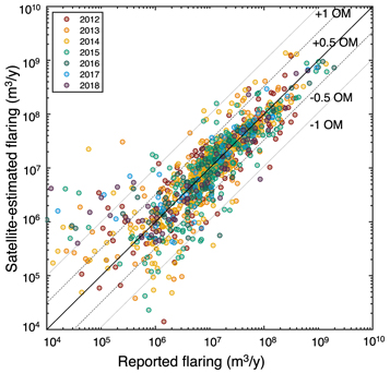
Figure 1. Comparison of satellite-estimated flaring rate to reported flaring rate [m3 y−1]. Where specified, standard cubic meters are used. Color represents year, with no significant trend in error across years found. Mis-alignment of satellite flaring estimate from reporting flaring rate could be due to mis-estimation of flare volume or mis-reporting of flaring emissions.
Download figure:
Standard image High-resolution imageNote that one cannot conclude that error between reported volumes and estimated volumes shown in figure 1 is entirely due to satellite error, as mis-reporting to governments or database errors could exist. Also, some misalignment between a flare and the associated field from which it is obtaining gas may occur. Without controlled release experiments where an independent entity is flaring metered quantities of gas, some ambiguity in the source of the error is unavoidable.
These results are reported separated by country in figure 2, with all years for each country represented in a single color for simplicity. We see that countries have quite different OM of flaring rates, with US and Norwegian flares skewing to the smaller range of our data and Brazil, Mexico, and Nigeria skewing toward the larger size scale. Because relative error in measurement is larger at smaller flaring rates (see figure 1 lower left), countries with smaller flare rates show more dispersion.
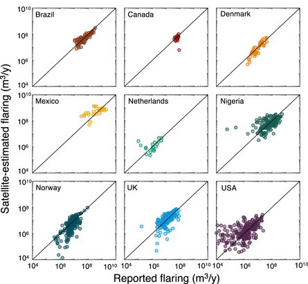
Figure 2. Flaring estimate accuracy by country. Errors tend to be larger at smaller scales, resulting in larger errors for countries with flaring rates skewed low (e.g., USA, Norway).
Download figure:
Standard image High-resolution imageNext we take the ratio of the satellite-estimated flaring volume to the government-reported volume for each matched flare (r = E/A, where E is m3 estimated via satellite and A is actual reported flared m3). We examine the distribution of these ratios by binning them into size classes of width 1 OM (see figure 3) for the main observations. The skewed distribution of the absolute ratios (top, panels a-c) is corrected to an approximate normal distribution by taking the log10 of the ratios (bottom, panels d-f).
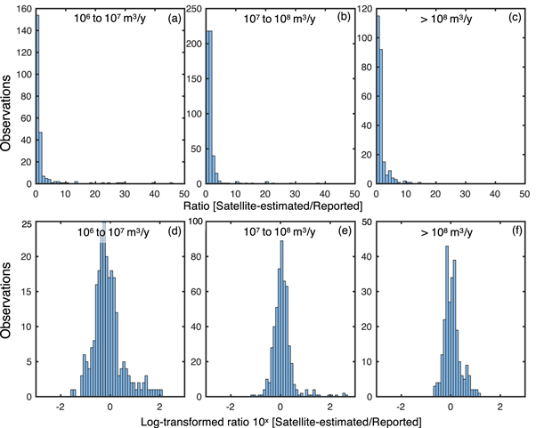
Figure 3. Distributions of ratios for 3 main size classes of width 1 OM. Top distributions (panels (a)–(c)) are highly skewed, which is corrected by taking the logatrithm of the ratio (panels (d)–(f)).
Download figure:
Standard image High-resolution imageContinuing to work with log10 transformed ratios, the box-and-whisker plot of figure 4 shows the distribution of flaring ratio volumes for each size class, with the scale on the y-axis representing the power-of-10 scale of the ratio (i.e., 1 = 101 or a r = 10, while −1 = 10−1 r = 0.1). We see that the size estimates for the smallest flares (size classes <104) are biased low: the ratios are skewed heavily to negative orders. In contrast, the central behavior for the largest size class (>108 m3 y−1) is accurate but the box is skewed high, with more spread in observations above the 1:1 ratio line. In moderate size classes the central estimates of the ratios grow as a function of size, and the skew is larger in the positive direction (larger whisker and more outliers).
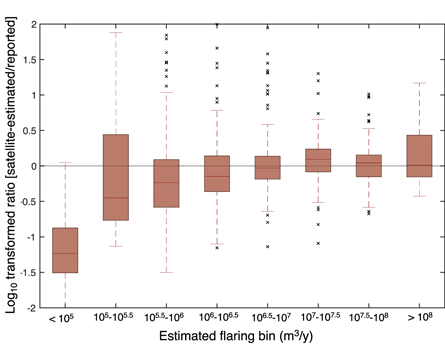
Figure 4. Box-plot of distribution of ratios of log10 transformed estimated/reported emissions, as a function of reported emissions rate. Bins are of size 10^0.5. Note log scale of y-axis.
Download figure:
Standard image High-resolution imageThe properties of these bins are given in table 3. The skew in ratios toward positive magnitudes suggests that ratios may be logarithmically distributed. We test for this by testing log-transformed ratios for normality using the one-sample Lilliefors test for normality. The Lilliefors test is a modification of the one-sample Kolmogorov-Smirnov (K-S) test that is appropriate when testing for the normality of a dataset in which the mean and SD of the distribution are not known a priori but must be estimated from the data. In all cases, the normality hypothesis is supported at a critical p-value threshold of 0.01.
Table 3. Properties of ratios of flare size estimates per bin of flare size (binned by satellite estimated flare size). Lillefors test performed using MATLAB statistics toolbox, using iterative approach with Monte Carlo convergence tolerance of 1e-4.
| Estimated flare size range [m3 y−1] | Counts [flares] | Ratios [estimated m3/reported m3] | Log-transformed ratios [log10(estimated/reported)] | Lillefors normality test for log-transformed ratios | ||||||
|---|---|---|---|---|---|---|---|---|---|---|
| Low | High | Clean Obs. | Median | Mean | SD | Median | Mean | SD | Lognormal? | p-value |
| 0 | 105 | 13 | 0.06 | 0.23 | 0.35 | −1.18 | −0.99 | 0.54 | 0 | 0.135 |
| 105 | 105.5 | 36 | 0.36 | 4.32 | 12.96 | −0.44 | −0.16 | 0.78 | 1 | 0.017 |
| 105.5 | 106.0 | 99 | 0.58 | 3.76 | 11.01 | −0.23 | −0.16 | 0.68 | 1 | 5.8e-5 |
| 106 | 106.5 | 140 | 0.71 | 3.41 | 13.24 | −0.15 | −0.05 | 0.53 | 1 | ~0 |
| 106.5 | 107 | 224 | 0.94 | 6.73 | 41.55 | −0.03 | 0.05 | 0.48 | 1 | ~0 |
| 107 | 107.5 | 292 | 1.24 | 3.22 | 23.29 | 0.09 | 0.09 | 0.33 | 1 | ~0 |
| 107.5 | 108 | 164 | 1.10 | 1.31 | 1.35 | 0.04 | 0.01 | 0.28 | 1 | 1.0e-3 |
| 108 | Max | 86 | 1.03 | 2.16 | 2.48 | 0.01 | 0.14 | 0.38 | 1 | 1.8e-4 |
These logarithmically distributed ratios suggest a model for generating the uncertainty range of expected reported volume of a satellite-observed flare. We do not know the actual flaring rate A in most cases (m3 y−1), but must estimate it from the satellite estimated rate E:

Where r represents a single realization of the ratio between satellite-observed and reported emissions (satellite/reported) and E is the satellite-estimated emissions rate [m3 y−1]. In uncertainty analysis, r can be drawn many times in a bootstrap approach.
The ratio factor r can be computed for each flare uncertainty realization by drawing a parameter d from a normal distribution N with μ and σ given above in table 3 depending on the size class estimated from the satellite:

The resulting ratio r for a given realization of d is then simply:

which can then be used to generate a series of realizations for actual flaring rates A given E. Note that because the above parameters are derived for offshore flaring, it is not clear how applicable they will be to onshore flare uncertainty estimation.
The decrease in relative error as a function of observation size seen above in figures 1 and 4 could be due to two effects. One is the larger absolute size of the flare, which would result in a larger flux of energy from the flare body and a stronger IR signal at the satellite, potentially enabling a more accurate estimate of flare volume. Second, larger observations are in some cases the result aggregation of multiple flares into a single estimate, such as fields or platforms with multiple flares, or in the extreme case of Mexico, where flares from multiple fields are aggregated into a single estimate for a producing region (required due to flaring reporting at the producing region). In order to test the relative effect of flare number aggregation versus flare size, we perform an analysis of the SD of ratio r for flare-groups created by randomly aggregating between 1 and 200 flares. A total of 106 aggregated groups of flares are created, and the ratio r for each aggregated flare grouping is recorded, along with the total amount of flaring in the grouping and the number of flares aggregated.
As we see in figure 5, the SD of the ratio within a size-number bin (box) decreases as the number of flares in a group increases (vertical) as well as when the total flared volume increases (horizontal). That is, summing more flares (moving up in plot) and summing larger flares (moving right in plot) both reduce dispersion of ratios r = E/A. We see a steeper dropoff in SD in the vertical direction, suggesting that summation of multiple flares into one grouping has a larger effect on ratio SD than absolute flare size.
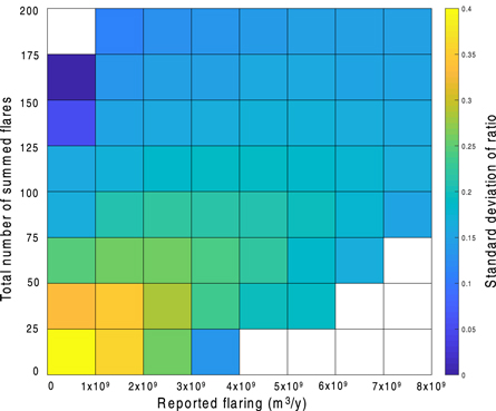
Figure 5. Change in SD of ratio r=E/A for aggregations of flares of a given number of flares (y-axis) and aggregation total flare size (x-axis). Higher SD in ratio r for a given box implies more dispersion in the estimate of ratios r for aggregated groups in that box.
Download figure:
Standard image High-resolution imageCountry-level uncertainty relationships could also be computed, i.e., compute distribution of values of R for each country. This would allow, perhaps, more accurate country-level uncertainty analysis for future estimates for that country. On the other hand, it would limit the generalization of the ratio distributions for R to other countries. Given the variety of regulatory and reporting regimes in our countries, we might expect that grouping across countries would allow better generalization power.
The above analysis focuses on estimating the actual flaring rate A in m3 y−1 for a flare with satellite-observed quantity E in m3 y−1. What about estimates for a whole region, or for the industry as a whole? While significant error exists at the individual flare level, as shown in figure 2, we can expect that much of this error will be compensated for when computing the total flaring in a large region, country, or globe. Figure 6 shows the total ratio of satellite-estimated volumes divided by reported volumes for each country in each year (body of table). It also shows the sum of all flares for a country across all years (right summary row), the sum of all flares for a year across all countries (bottom summary row), and all flares in all countries (bottom-right, entire dataset, N = 1054).
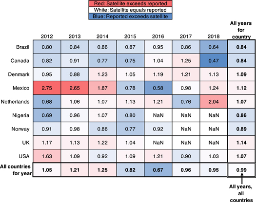
Figure 6. Ratio of satellite-estimated flaring rate to reported flaring rate by country and year. Summary rows on right and bottom report sums across years and countries respectively. Ratio at bottom-right is all 1054 observations, equal to 0.9898.
Download figure:
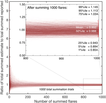
Standard image High-resolution imageTo illustrate this more generally, we show the impacts of sequential summation in figure 7 below. We choose a flare at random from the dataset (with replacement) and add it to the cumulative sum of each of the reported volume and the satellite-estimated volume. We do this for 1 to 1000 flares, showing that if one sums a small number of flares the variance is wide, but by the time we sum 1000 flares, the bias is minimal (mean ratio at 1000 flares cumulatively summed is 0.992) and dispersion is small (25%–75%ile range is 0.943 to 1.034).
Figure 7. Reduction in dispersion of ratio of cumulative satellite-estimated flaring rate to government-reported flaring rate as the number of summed flares increases. 1000 total trials were performed.
Download figure:
Standard image High-resolution image
This suggests that the estimated flaring rate for global offshore oil and gas operations is likely quite close to the actual flaring rate, given that the global estimate is derived from summing 1000 s of offshore flares in countries around the world. Given the results of figure 7, totals of offshore flaring in the VIIRS datasets can be expected to be 2σ-accurate at approximately +/−5%.
We cannot comment, based on these results, on the accuracy of land-based flaring estimates, as the physics of observation may differ between land and ocean-based observations. The reflective/emissive character of surrounding water and vegetation/soil presumably differ enough to warrant a separate examination of land-based flare estimates. Also, differences in atmospheric transmission above oceans and land may differ systematically (i.e., cloud cover, haze and aerosol, other pollution). This suggests that future work should examine land-based flaring rates.
This study also cannot offer insights into venting or purposeful release of methane. Because the IR satellites used to generate flare images, and thereafter flare volume estimates, are sensitive to radiation in the near-IR, they are not useful for sensing venting of methane. Some satellite methane estimates have been generated, and there is significant interest in developing remote sensing of methane emissions estimates from remote sensing platforms. Assessing the accuracy of such methods is important future work.
Determining minimum detection thresholds and confusion matrices (i.e., true positive, false positive rates) is in theory possible with these datasets, and should be pursued in future work. Such analysis may be challenged by incomplete reporting (e.g., reporting occurs only above a threshold), by sporadic flares which do not meet significance cutoffs in the VIIRS product for number of observations per year but are nonetheless real, or by operations that are mobile or temporary, such as process upset or drilling-and-completion flares.
More importantly for long-run usefulness of these data is the need for independent controlled ground tests. Because of possible errors, bias, or fraud in reporting, independent controlled ground flaring events would provide valuable data for improving future algorithms.