
Abstract
We develop an algorithm for i) computing generalized regular  -point grids, ii) reducing the grids to their symmetrically distinct points, and iii) mapping the reduced grid points into the Brillouin zone. The algorithm exploits the connection between integer matrices and finite groups to achieve a computational complexity that is linear with the number of
  -points. The favorable scaling means that, at a given
  -point density, all possible commensurate grids can be generated (as suggested by Moreno and Soler) and quickly reduced to identify the grid with the fewest symmetrically unique
  -points. These optimal grids provide significant speed-up compared to Monkhorst–Pack
  -point grids; they have better symmetry reduction resulting in fewer irreducible
  -points at a given grid density. The integer nature of this new reduction algorithm also simplifies issues with finite precision in current implementations. The algorithm is available as open source software.
Export citation and abstract BibTeX RIS
1. Introduction
Codes that solve the many-body problem using density functional theory (DFT) use uniform grids over the Brillouin zone in order to calculate the total electronic energy, among other material properties. The total electronic energy is calculated by numerically integrating the occupied electronic bands. For metallic systems, there exist surfaces of discontinuities at the boundary between occupied and unoccupied states, collectively known as the Fermi surface. These discontinuities cause the accuracy in the calculation of the total electronic energy to converge extremely slowly and erratically with respect to grid density. This is demonstrated in figure 1 where we compare the convergence of an insulator (silicon) with a metal (aluminum).

Figure 1. Total energy error versus  -point density for the cases of silicon and aluminum. Silicon does not have a Fermi surface so there is no discontinuity in the occupied bands; convergence is super-exponential or
  where n is the number of
  -points. (See the discussion of example 1 in [1].) In contrast, the total energy of aluminum converges very slowly, and the convergence is quite erratic. For typical target accuracies in the total energy, around 10−3 eV/atom, metals require 10–50 times more
  -points than semiconductors.
Download figure:
Standard image High-resolution imageThe poor convergence of the electronic energy means that DFT codes must use extremely dense grids [2, 3] to achieve an accuracy of several meV/atom. To reduce computation time, it is common practice to evaluate eigenvalues at symmetrically equivalent  -points only once. This is the essence of 'symmetry reducing' a
  -point grid.
In most DFT codes, even for very dense grids, the setup and symmetry reduction of the grid takes a few seconds at most. Our motivation for an improved algorithm (despite the speed of current routines) is two-fold: 1) enable an automatic grid-generation technique that allows us to scan over thousands of candidate grids, in a few seconds, to find one with the best possible symmetry reduction [4, 5] (in other words, enable a  -point generation method in the same spirit as that of [2] but have the grid generation done on-the-fly [6]), and 2) eliminate (or at least greatly reduce) the probability of incorrect symmetry reduction3
as the result of finite precision errors (the danger of these increases as the density of the integration grid increases).
-point generation method in the same spirit as that of [2] but have the grid generation done on-the-fly [6]), and 2) eliminate (or at least greatly reduce) the probability of incorrect symmetry reduction3
as the result of finite precision errors (the danger of these increases as the density of the integration grid increases).
In this brief report, an algorithm for generating, and subsequently symmetry-reducing,  -point grids is explained. This algorithm builds on concepts such as Hermite Normal Form, Smith Normal Form, and the connection between finite groups and integer matrices. These concepts are briefly explained in the main text; for more details, see the appendix and [8]. The algorithm has been implemented in an open-source code available at https://github.com/msg-byu/kgridGen and incorporated in version 6 of the VASP code [9]. The algorithm has been incorporated into a code for generating generalized regular grids https://github.com/msg-byu/GRkgridgen [6].
2. Generating grids
As demonstrated in figure 3, every uniform sampling of a reciprocal unit cell can be expressed through the simple integer relationship

where  , and
, and  are 3 × 3 matrices; the columns of
  are the reciprocal lattice vectors, and the columns of
  are the
  -point grid generating vectors. Put simply,
  describes the integer linear combination of vectors of
  that are equivalent to
  . One obtains Monkhorst–Packgrids (regular grids) when
  is an integer, diagonal matrix. More generally, when
  is an invertible, integer matrix, one obtains generalized regular grids. Examples of Monkhorst–Packand generalized regular grids are given in figure 2. We use R to refer to the infinite lattice of points defined by integer linear combinations of
  , and K to refer to the lattice of points defined by
  .
.

Figure 2. Two-dimensional example of a Monkhorst–Packgrid (a) and a generalized regular grid (b). The two grids have the same  -point density, but different grid-generating vectors
  and
and  . Both grids are commensurate with the reciprocal unit cell, shown as a black square. For Monkhorst–Packgrids, the matrix
  in equation (1) is integer and diagonal. In contrast, for generalized regular grids,
  is not necessarily diagonal but is any invertible integer matrix.
Download figure:
Standard image High-resolution image
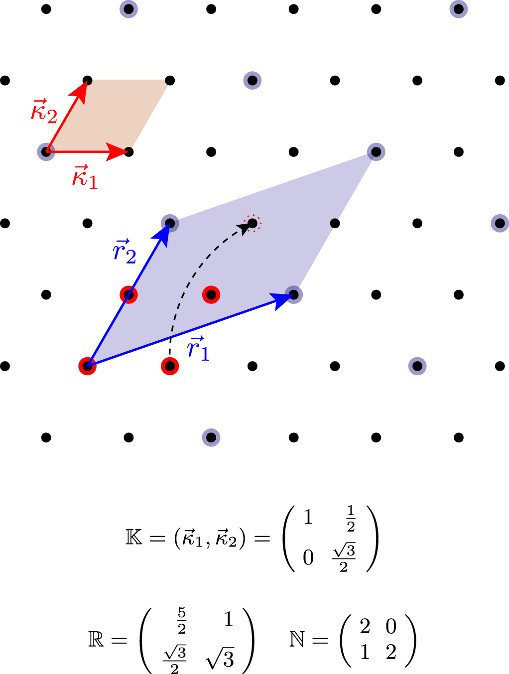
Figure 3. An example of the integer relationship between the reciprocal lattice vectors  and the grid generating vectors
  . In the picture, the grid generating vectors,
  and
and  , the columns of
  , define a lattice of points, four of which are inside the unit cell (blue parallelogram) of
  . Note that in the most general case, the relationship between the two lattices,
  need not be diagonal (as it is for Monkhorst–Pack [10]
  -point grids.)
Download figure:
Standard image High-resolution imageWith no loss of generality, a new basis for the lattice K can be chosen (a different, but equivalent,  ) so that
  is a lower triangular matrix in Hermite normal form (HNF) [11]. (See section II-A of [8] for a brief introduction to HNF.) HNF is a lower-triangular canonical matrix form, where the entries below the diagonal are non-negative and strictly less than the diagonal entry in the same row. Code for converting integer matrices to Hermite Normal Form is available at https://github.com/msg-byu/symlib in the rational_mathemematics module.
A  -point integration grid is the set of points of the lattice K that lie inside one unit cell (one fundamental domain) of the reciprocal lattice R. We refer to this finite subset of K as Kα (See figure 3; black dots are K, dots inside the blue parallelogram comprise Kα.) The number of points that lie within one unit cell of R is given by
  .
.
How then does one generate these n points? If  is in HNF, then the diagonal elements of
  are three integers, a, c, and f, such that a · c · f = n. A set of n translationally distinct4
points of the lattice K can be generated by taking integer linear combinations of the columns of
are three integers, a, c, and f, such that a · c · f = n. A set of n translationally distinct4
points of the lattice K can be generated by taking integer linear combinations of the columns of  :
:

where p, q, and r are nonnegative integers such that

The n points generated this way will not generally lie inside the same unit cell, but they can be translated into the same cell by expressing them in 'lattice coordinates' (fractions of the columns of  , instead of Cartesian coordinates) and then reducing the coordinates modulo 1 so that they all lie within the range
  . This is illustrated by the dashed arrow in figure 4.

Figure 4. An example of generating the points of K (black lattice) that lie within one unit cell (blue parallelogram) of the lattice R (blue lattice). The lattice K is generated by the basis  (columns of
  ). The four points of Kα are generated by
  , where 0 ≤ m1 < 2,
  . Note that the upper limits of m1 and m2 are the diagonals of
  when it is expressed in HNF.
Download figure:
Standard image High-resolution imageExpressed as fractions of the lattice vectors of R, these four points are:

Initially,  is not in the same unit cell as the other three points; its first coordinate is not between 0 and 1. After reducing the first coordinate modulo 1,
  moves to an equivalent position in the same unit cell as the other three points.
In summary, this first part of the algorithm generates n translationally distinct points and translates them all into the first unit cell of R. (It is not necessary to translate all the points into the first unit cell, but it is convenient to do so as a first step to translating them into the first Brillouin zone. The translation into the first Brillouin zone is less trivial and is discussed in section 4.)
3. Symmetry reduction of the grid
In many cases the crystal will have some point group symmetries, and these can be exploited to reduce the number of  -points where the energy eigenvalues and corresponding wavefunctions need to be evaluated. The grid is reduced by applying the point group symmetries5
of the crystal to each point in the grid. For example, in figure 5, the points connected by green arrows will be mapped onto one another by successive 90° rotations. These four symmetrically equivalent points lie on a 4-fold 'orbit' (as do the points marked by the red arrows). The point at the origin maps onto itself under all symmetry operations and has an orbit of length 1.
-points where the energy eigenvalues and corresponding wavefunctions need to be evaluated. The grid is reduced by applying the point group symmetries5
of the crystal to each point in the grid. For example, in figure 5, the points connected by green arrows will be mapped onto one another by successive 90° rotations. These four symmetrically equivalent points lie on a 4-fold 'orbit' (as do the points marked by the red arrows). The point at the origin maps onto itself under all symmetry operations and has an orbit of length 1.

Figure 5. An example of symmetry reducing a grid. The reciprocal unit cell is the blue square. This example assumes that the wavefunctions have square symmetry (the D4 group, 8 operations). The example grid is a 3 × 3 sampling of the reciprocal unit cell. The point at (0,0) is not equivalent to any of the other eight points. There are two sets of equivalent points, each set with 4 points in the orbit, connected by red and green arrows, respectively. The points marked by red arrows are equivalent under horizontal, diagonal, and vertical reflections about the center of the square. The green-marked points are equivalent by 90◦ rotations. Thus the nine points are reduced (or 'folded') into three symmetrically distinct points.
Download figure:
Standard image High-resolution imageFor a grid containing Nk points and a group (of rotation and reflection symmetries) with NG operations, a naive algorithm for identifying the symmetrically equivalent points and counting the length of each orbit would be as follows: For each point ( loop), compare all rotations of that point (a loop of
  ) to all other points (another
  loop) to find a match; for a total computational complexity of
  . The algorithm is shown in pseudocode in figure 6. NG will never be larger than 48, but Nk may be as large as 503 for extremely dense grids, so the
  complexity of this naive approach is undesirable. But using group theory concepts (see the appendix for details), we can construct a hash table for the points that reduces the complexity from
  ) to
) to  by eliminating the kj loop in algorithm 1. The hash table makes a one-to-one association between the ordinal counter (the index) of each point and its coordinates.

Figure 6. The typical algorithm for reducing a grid by symmetry. In the algorithm, uniqueCount is a running counter of the number of unique points and serves as the index of the orbit, First is a list of the indices of the unique points, Wt (weight) is the number of symmetrically equivalent versions of each  -point in First, unique is an array of ones and zeros where each element corresponds to a
  -point in Kα. An element gets set to zero when the corresponding
  -point is equivalent to another
  -point, or when the
  -point becomes the representative
  -point of an orbit. This algorithm scales quadratically with the number of points in Kα and requires floating point comparisons between
  and
and  .
.
Download figure:
Standard image High-resolution imageThe three coefficients p, q, r in equation (2) can be conceptualized as the three 'digits' of a 3-digit mixed-radix number pqr or as the three numerals shown on an odometer with three wheels. The ranges of the values are 0 ≤ p < d1, 0 ≤ q < d2, and 0 ≤ r < d3, where d1, d2, d3 are the 'sizes' of the wheels, or in other words, the base of each digit. Then the mixed-radix number is converted to base 10 by

The total number of possible readings of the odometer is  . So it must be the case that the number of
  -points in the cell is
  . Each reading on the odometer is a distinct point of the n points that are contained in the reciprocal cell. Via equation (3) it is simple to convert a point given in 'lattice coordinates' as (p, q, r) to a base-10 number x. The concept of the hash table is to use this base-10 representation as the index in the hash table. Without the hash table, comparing two points is an
  search because one point must be compared to every other point in the list to check for equivalency. But with the hash function, no search is necessary—one simply maps the point (p, q, r) to the index x of the equivalent
  -point in the hash table.
It is not generally the case that the coefficients p, q, r for every interior point of the unit cell obey conditions:

(Figure 4 shows an example where the interior points do not meet these conditions.) These conditions hold only for a certain choice of basis. That basis is found by transforming the matrix  in equation (1) into its Smith Normal Form [11],
  . By elementary row and column operations, represented by unimodular matrices
  and
and  , it is possible to transform
  into a diagonal matrix
  , where each diagonal element divides the ones below it:
  , and
, and  (the notation
  means that i is divisible by j). As explained in the appendix (section A.1), when
  is expressed in Smith normal form (SNF) and the interior points of the reciprocal cell are expressed as linear combinations of the grid generating vectors
  , then the coordinates (coefficients) of the interior points will obey equation (4). When these conditions are met, the hashing algorithm discussed above (in particular, equation (3)) becomes possible. This enables the
  algorithm, shown in figure 7.

Figure 7. Our algorithm that reduces a grid to a set of symmetrically distinct  -points. In the algorithm, uniqueCount is a running counter of the number of unique points and serves as the index of the orbit, First is a list of the indices of the unique points, Wt (weight) is the number of symmetrically equivalent versions of each
  -point in First, and hashtable is a hash table that points from the position of a
  -point in Kα to the index of its orbit. In contrast to algorithm 1, this algorithm scales linearly with the number of points in the grid Kα and does not require floating point comparisons.
Download figure:
Standard image High-resolution image4. Moving points into the first Brillouin zone
For accurate DFT calculations, it is best if the energy eigenvalues (electronic bands) are evaluated at  -points inside the first Brillouin zone, so our algorithm includes a step that finds the translationally equivalent grid points in the Brillouin zone. (In principle, the electronic structure
  should be the same in every unit cell, but numerically the periodicity of the electronic bands is only approximate, becoming less accurate for
  -points in unit cells farther from the origin.)
The first Brillouin zone of the reciprocal lattice is simply the Voronoi cell centered at the origin—all  -points in the first Brillouin zone are closer to the origin than to any other lattice point. Conceptually, an algorithm for translating a
  -point of the integration grid into the first zone merely requires one to look at all translationally equivalent 'cousins' of the
  -point and select the one closest to the origin. But the number of translationally equivalent cousins is countably infinite, so in practice, the set of cousins must be limited only to those near the origin.
How can we select a set of cousins near the origin that is guaranteed to include the closest cousin? The key idea is illustrated in two-dimensions in figure 8. In three-dimensions, if the basis vectors of the reciprocal unit cell are as short as possible (the so-called Minkowski-reduced basis [12]), then the eight unit cells that all share a vertex at the origin must contain the Brillouin zone. In other words, the boundary of this union of eight cells is guaranteed to circumscribe the first Brilloun zone (i.e., the Voronoi cell containing the origin). A proof of this '8 cells' conjecture is given in the appendix (section A.1). The steps for moving  -points into the Brillouin zone are as follows:
- 1.
- 2.For each
 -point in the reduced grid, find the translation-equivalent cousin in each of the eight unit cells that have a vertex at the origin.
 - 3.From these eight cousins, select the one closest to the origin.


Figure 8. A two-dimensional example of the 'closest cousin' guarantee. The Brillion zone (blue) will be completely contained in the union of 4 basis cells around the origin (shown in red) when the basis vectors are chosen to be as short as possible (the so-called Minkowski basis). On the other hand, if the basis is not Minkowski reduced, regions of the Brillouin zone may lie outside the union of the 4 basis cells (depicted by the cell in green). A proof is given in the appendix (section A.1).
Download figure:
Standard image High-resolution image5. Conclusion
We have developed an algorithm that i) generates generalized regular  -point grids, ii) reduces the grids by symmetry, and iii) maps the points of the reduced grids into the first Brillouin zone. Whereas the typical algorithm for generating and reducing
  -point grids scales quadratically with the number of
  -points, this algorithm scales linearly. The improved scaling becomes essential when one generates and symmetry reduces all combinatorically possible generalized regular grids at a given
  -point density, in order to select the one with the fewest number of reduced
  -points [6].
The algorithm is also useful because it relies primarily on integer-based operations, making it more robust than typical floating point-based algorithms that are prone to finite precision errors. Mapping the grid to the first Brillouin zone is more efficient due to a proof that limits the search for translationally equivalent  -points to the eight unit cells having a vertex at the origin. The algorithm has been incorporated into version 6 of VASP [9].
Acknowledgments
We are grateful to Martijn Marsmann who found a bug in an early version of the code that spoiled the  scaling and who implemented the algorithm in VASP, version 6. Tim Mueller also contributed by pointing out a simpler approach to generating all the
  -points interior to the unit cell of R than we originally proposed. GLWH, WSM, and JJJ are grateful for financial support from the Office of Naval Research (MURI N00014-13-1-0635).
Appendix
A.1. Proof limiting Brillouin zone location
Given a point x in the space, we will use the term cousin for a point  which differs from x by an element of the lattice—i.e., a coset representative or a lattice-translation equivalent point.
Let R be a basis. Let UR denote the union of 2d basis cells around the origin—the set of points which are expressible in terms of the basis R with all coefficients having absolute value < 1. Let V denote the Voronoi cell (Brillouin zone)—the set of all points in the space which are closer to the origin than any other lattice point. Note that UR depends on the basis R, but V depends only on the lattice. Note also that both UR and V are convex sets.
We claim (in two and three dimensions) that if R is a Minkowski basis, then  . We shall argue by contrapositive— if
  , then the basis is not Minkowski reduced.
If  then V must intersect the boundary of UR, so there exist points on the boundary of UR which are closer to the origin than to any other lattice points. Equivalently, those points are closer to the origin than any of their cousins.
Note that among the cousins of any point on the boundary of UR, there is always a closest to the origin. But usually points on the boundary will have closer cousins in the interior. But if  there must be points on the boundary which have no closer cousins in the interior of UR. In other words, there are points (at least one) on the boundary such that all of its cousins in the interior of UR are farther from the origin.
A.1.1. 2D argument
Let  and
and  be basis elements of R. Assuming that
  there must be a point x on the boundary of UR whose cousins are all farther from the origin than x.
Without loss of generality (re-label the basis if necessary), we may express one of the bounding edges of UR as  where λ ∈ [−1, 1]. One of its interior cousins is
  , which is illustrated in figure A1. We have (since
  must be farther from the origin)

Since the expression on the left-hand side is greater than zero, the expression on the right-hand side must be also and taking the absolute value of both sides does not change the inequality:

Considering the worst case scenario of λ = 1 gives

which violates the condition of a Minkowski basis  . The remaining three boundaries are similar to the one just considered, the only differences being permutations of the basis elements
  and
and  and possibly changes of sign. When applying the same reasoning to the other edges we arrive at the same contradiction. Hence, the points on the boundary of UR are closer to the origin than interior cousins,
  , only when the basis R is not Minkowski reduced. If R is Minkowski reduced, all points on the bounday of UR have interior cousins that lie closer to the origin and
  .
.

Figure A1. Each point along the boundary of UR has at least one interior cousin closer to the origin when R is Minkowski reduced. For the points along the edge in red, these interior cousins are the points along the dashed red line.
Download figure:
Standard image High-resolution imageA.1.2. 3D argument
Let  , and
, and  be the basis elements of R, and suppose (relabeling the basis vectors if necessary) that
  (where λ and δ are elements of [−1, 1]) is a point on the boundary of UR which is closer to the origin than are its interior cousins.
One of those cousins is a plane through the origin  . The boundary and cousin planes are shown in figure A2. Thus

Simplifying this expression gives

Since the expression on the left-hand side is greater than zero, the expression on the right-hand side must be also and taking the absolute value of both sides does not change the inequality:


Figure A2. Each point along the boundary of UR, the edges of which are shown in black, has at least one interior cousin closer to the origin when R is Minkowski reduced. For the points on the bounding plane in red, the interior cousins are the points on the plane in blue. (The origin is contained in the blue plane.)
Download figure:
Standard image High-resolution imageTo simplify the right-hand side of equation (7) the triangle inequality is used, making it more likely that the inequality is satisfied:

Since the expression in equation (8) does not depend on the sign of λ or δ, we can restrict λ and δ to positive values within [0,1] without loss of generality. Consider now another cousin that lies within UR and on the same plane as  :
:  . Repeating the same process for
  with
with  gives
gives

Combining equations (8) and (9) gives

Assuming  forms a Minkowski basis, and plugging in the largest possible values for all quantities under this assumption on the right-hand side of equation (10) gives the contradiction
  . The remaining seven bounding planes are similar to the one just considered, the only differences being permutations of the basis elements
  ,
,  , and
, and  and changes of sign. We arrive at the same contradiction when applying the same reasoning to the other planes. Hence, the points on the boundary of UR are closer to the origin than interior cousins,
  , only when the basis R is not Minkowski reduced. If R is Minkowski reduced, all points on the boundary of UR have interior cousins that lie closer to the origin and
  .
.
A.2. Groups, matrices, and lattices in smith normal form
The discussion below is limited to three-dimensions though the arguments easily generalize to higher dimensions. The purpose of the discussion below is to help the reader make the connection between groups and integer matrices. The Smith Normal Form is a key concept to make this connection.
In this discussion, we show that we can associate a single, finite group with the lattice sites within one tile (i.e., one unit cell) of a superlattice. In our application, this tile is the unit cell of the grid generating vectors and the superlattice is the reciprocal cell. The association between the group and the lattice sites is a homomorphism that maps each lattice site to an element of the group. If two points are translationally equilavent (same site but in two different tiles) they will map to the same element of the group. This homomorphism is the key ingredient to constructing the hash function (see equation (3)) that enables a perfect hash table where points are listed consecutively, from 1 to N. In what follows, we explain in detal how this association is made, i.e., we detail how one finds this homomorphism.
A.2.1. Groups in smith normal form
Begin with the simplest case. Let  be a non-singular 3 × 3 matrix of integers. Its columns represent the basis for a subgroup
  of the group Z3 (where Z is the set of all integers, and the group operation is addition). The two latttices whose symmetries are represented by these two groups are the 'simple cubic' lattice of all points with all integer coordinates and its superlattice7
whose basis is given by the columns of
of the group Z3 (where Z is the set of all integers, and the group operation is addition). The two latttices whose symmetries are represented by these two groups are the 'simple cubic' lattice of all points with all integer coordinates and its superlattice7
whose basis is given by the columns of  . Since Z3 and its subgroups are Abelian, we know that all the subgroups are normal so there exists a quotient group
  , and that group is finite.
Note that the cosets which form the elements of that quotient group are simply the distinct translates of the lattice  within Z3. In fact, each coset has exactly one representative in each unit cell, so the order of G is equal to the volume of a unit cell (the absolute value of the determinant of
  ). Since the quotient group G is finite, and Abelian, it must be a direct sum of cyclic groups (by the Fundamental theorem of Finite Abelian Groups).
One canonical form for direct sums of groups is called Smith Normal Form, where the direct summands are ordered so that each summand divides the next. In other words,  where
where  and (of course)
  . Any finite Abelian group can be uniquely written in this form. (Isomorphic groups will yield the same 'invariant factors' m1, m2,...,mk when written in this form.)
Note that, since  , there must be a homomorphism from Z3 onto G, having
  as its kernel. In other words,
  . Our task is to find the direct-sum representation of the quotient group
  , and also to find the homomorphism ψ which maps the points of Z3 onto the group (in such a way that ψ(p) = 0 iff
  ). This allows us to work with the elements of the group as proxies for the
  -points inside the reciprocal cell.
A.2.2. Matrices in smith normal form
There is a useful connection between the SNF for Abelian groups and the SNF for integer matrices. As the reader may infer, the SNF form of the basis matrix  effectively tells one how to represent the quotient group
  as a direct sum of cyclic groups in Smith Normal Form, and, as shown in the following section, the row operations used to create the SNF of
  give the homomorphism ψ suggested above.
A.2.3. The connection between SNF groups and SNF matrices
In the matrix case, since the operations are elementary row and column operations, we have  where
where  and
and  are integer matrices with determinant ±1 representing the accumulated row operations and column operations respectively. The matrix
  is completely determined by
  , but the matrices
  and
and  depend on the algorithm used to arrive at the Smith Normal Form of
  . A different implementation might yield
  (same
(same  and same
  , but different
  and
and  ).
).
Note that, since  represents elementary column operations, the product
  simply represents a change of basis from
  to a new basis
  . In other words, the columns of
  are still a basis for
  . But the new basis has the property that
  . That means that every element
  of
of  (where
  is some element of
  ) will satisfy the equation
  . In other words,
  will be a vector whose entries are multiples of the corresponding diagonal entries in
  .
.
To put it another way, define  to be the operation that maps
  in
in  to
to  .
.
Then we have shown  iff
iff  (the zero-element in the group
  .
.
That suggests we let  , a homomorphism from Z3 onto the direct-sum G0. Then, since that homomorphism is easily shown to be onto, and its kernel is
  , we see (by the First Isomorphism theorem of group theory) that
  , and ψ is precisely the homomorphism we sought.
Thus we have connected the two versions of SNF. The matrix algorithm provides the SNF description of the quotient group by the diagonal entries in  , and the transition matrix
  provides the homomorphism which maps the parent lattice onto the group.
A.2.3.1. An example
Let  . This describes a lattice
  which contains the points
  , and
, and  , and all the points which are integer linear combinations of those three points. The matrix
  has determinant 12, which must be the volume of each lattice tile—and it is also the order of the quotient group
  .
.
Using the SNF algorithm to diagonalize this basis matrix, we find  where
where  , with
  and
and  .
.
Thus we now know that the quotient group is  .
.
Further, from the matrix  , we may obtain the homomorphism projecting Z3 onto the quotient group, with kernel
  . If
. If  then
then  and thus

(noting that anything mod 1 is zero).
Note that this homomorphism provides a different, but convenient, way to describe the superlattice. Since  is the kernel of ψ, it is comprised of the points (x, y, z) ∈ Z3 which satisfy the simultaneous congruences z ≡ 0 (mod 2) and
  (mod 6). We note that all three basis points p1, p2 and p3 satisfy these congruences, and thus so will all their integer linear combinations (all points in
  ).
).
A.2.3.2. Algorithmic variation
In the example we computed above, a different application of the SNF matrix algorithm, with the same  , might have yielded the same diagonal matrix
  , but different
  and
and  , which would change the homomorphism to
  (mod 2),
  (mod 6)) =
  ,
,  (mod 6)). The new homomorphism is different, since (1, 0, 1) ↦ (0, 5) now, where previously (1, 2, 3) ↦ (1, 5) (for example), but the kernel is the same. In fact the two homomorphisms are related via an automorphism of the group G.
A.2.4. Non-integer lattices
Now, what about the more complicated situation, where  represents a (possibly HNF) matrix describing the change from some lattice other than the simple integer lattice Z3 to one of its subgroups (superlattice)?
Then we have a basis  and lattice
  and a basis
  for a (super) lattice
  . Again, the quotient group
  is Abelian of order
  . Again, G is a direct sum of cyclic groups corresponding to the diagonal entries of
  (where
  is the SNF of
  ).
).
The only difference here is that the homomorphism ψ provided by  must depend on the basis
  (which might even be irrational). Every point in
  has the form
  where
where  is a column of integers. Then
  (modded by the corresponding entries from
  ). We could write it as
  (with the entries appropriately modularly reduced and transposed to a horizontal vector).
A.2.5. Example: general (non-integer) lattices
Suppose  is the lattice defined by (columns of) the basis matrix
  , and
, and  is the subgroup lattice defined by the basis marix
  where
where  . In other words, one basis for
  is given by the columns of
  .
.
Reducing  to SNF yields

Thus our quotient group is  and
and  so
so

which provides our homomorphism  from
from  onto G.
If we let  which is an element of
  but not of
  , then
  and
and  (after reducing the elements modulo 2, 2 and 4 respectively). On the other hand, if we let
  , which is an element of
  (the kernel), then
  and so
  , and
, and  is in the group.
By this function ψ, the elements of  are all mapped to elements of the group G and, in particular, the elements of
  are mapped to the zero element of the group. Stated in terms of the cosets, the entire set
  is mapped to the zero element of the group G, and each of the distinct translates of
  (within
  ) gets mapped to a different element of the group. We might think of this as decorating or labeling the elements of
  in a periodic manner, using
  to define the period, and using the elements of the group G as the labels.
Footnotes
- 3
Such errors are not uncommon in
-point reduction, but are not documented in the literature. The same errors are known to affect symmetry analysis as discussed at length in [7]. - 4
If two points are translationally distinct, their difference cannot be an integer linear combination of the reciprocal cell vectors; that is,
, for all integer values n, m, ℓ. ( are the columns of .) - 5
In addition to the rotations, reflections, and improper rotations of the crystal, inversion symmetry is also included by default. Even when the crystal itself does not have inversion symmetry, the electronic bands generally will. If, as in the case of magnetism, the inversion symmetry is broken, the inversion symmetry can be disabled in the code.
- 6
Our Fortran code for computing the Minkowski reduced basis is available at https://github.com/msg-byu/symlib in the vector_matrix_utilities module.
- 7
In the mathematical literature, and in some of the crystallography literature, these 'superlattices' are referred to as sublattices. The group associated with a 'superlattice' is a subgroup of the group associated with the parent lattice. Although this nomenclature (subgroups, sublattices) is more correct from a mathematical or group theory point of view, we follow the nomenclature typically seen in the physics literature where a lattice or a structure whose volume is larger than that of the parent is referred as a superlattice.


