

Abstract
Multiphoton fluorescence lifetime microscopy has revolutionized studies of pathophysiological and xenobiotic dynamics, enabling the spatial and temporal quantification of these processes in intact organs in vivo. We have previously used multiphoton fluorescence lifetime microscopy to characterise the morphology and amplitude weighted mean fluorescence lifetime of the endogenous fluorescent metabolic cofactor nicotinamide adenine dinucleotide (phosphate) (NAD(P)H) of mouse livers in vivo following induction of various disease states. Here, we extend the characterisation of liver disease models by using nonlinear regression to estimate the unbound, bound fluorescence lifetimes for NAD(P)H, flavin adenine dinucleotide (FAD), along with metabolic ratios and examine the impact of using multiple segmentation methods. We found that NAD(P)H amplitude ratio, and fluorescence lifetime redox ratio can be used as discriminators of diseased liver from normal liver. The redox ratio provided a sensitive measure of the changes in hepatic fibrosis and biliary fibrosis. Hepatocellular carcinoma was associated with an increase in spatial heterogeneity and redox ratio coupled with a decrease in mean fluorescence lifetime. We conclude that multiphoton fluorescence lifetime microscopy parameters and metabolic ratios provided insights into the in vivo redox state of diseased compared to normal liver that were not apparent from a global, mean fluorescence lifetime measurement alone.
Export citation and abstract BibTeX RIS
Introduction
Multiphoton microscopy with fluorescence lifetime imaging (MP-FLIM) enables deep, specific, quantitative and safe imaging of various organ sub-architecture and redox processes in vivo. We have now used MP-FLIM to study the pathophysiology and xenobiotic transport in a range of organs, including the liver, the kidney and the skin [1–17]. In this work, we have responded to requests to revisit previous work that examined changes in NAD(P)H and collagen using MP-FLIM with a focus on the liver to expand upon the analysis presented.
The analysis is important in the context of the liver being the key organ in the synthesis, metabolism and excretion of key endogenous and exogenous solutes, including being the key detoxifying organ for all solutes absorbed from the gastrointestinal tract. In particular, the liver processes carbohydrates, fats and proteins from the digestive tract to produce energy, metabolises and excretes into the bile various endogenous substrates, xenobiotics and their metabolites and can facilitate enterohepatic recirculation [18]. Hence, the liver plays a major role in ultimately regulating what is circulated to the rest of the body. We have shown that various liver diseases can compromise the liver's metabolic function and that the extent of impairment may be directly related to the severity of the liver disease and the nature of the solutes involved [19–21]. In these early studies, we used destructive sampling to assess the fate of different drugs in liver disease. In later studies, we began non-invasively imaging fluorescent drugs and their metabolites in the liver [2, 22]
It is now well known that the redox state and reactions of the liver are critical to metabolic and other functions of the liver and their modification by exogenous compounds and disease can impair liver function [23]. Whilst the autofluorescent intracellular coenzymes, reduced nicotinamide adenine dinucleotide (NADH) and flavin adenine dinucleotide (FAD), are key contributors to cell respiration and energy homeostasis, the autofluorescent reduced nicotinamide adenine dinucleotide phosphate (NADPH) is a key liver redox regulator involved in reductive biosynthesis and a cofactor involved in the glutathione scavenging of free radicals, heme-mediated P450 enzyme oxidation of many solutes [24, 25] and the flavin-containing monooxygenases (FMO) 2, 3, 4 and 5 catalyze the oxidation of various endogenous and exogenous solutes with amine, sulphur, and phosphorous groups [26]. Importantly, the autofluorescent fully oxidized (quinone form) coenzyme, FAD, which is reduced to its hydroquinone form, FADH2, is also involved in this later process. The reaction rate for NADH is usually several orders lower than that of NADPH [27]. However, NADH is a key source of NADPH and is generated by several enzymes in both the liver cytoplasm and mitochondria. The oxidised forms of NAD+ and NADP+, as well as the reduced FADH2, are not fluorescent. Glock and McLean [28] have reported NADP+, NADPH, NAD+ and NADH concentrations (μg g−1 tissue) of 425, 116, 25 and 231, respectively. Given that NADPH and NADH have identical fluorescence signatures and cannot be separated in MP-FLIM imaging [29], the two entities are collectively referred to here as NAD(P)H.
The metabolic cofactors NAD(P)H and FAD can also exist in both an unbound (free) form and in a protein bound form, with these forms having different fluorescence lifetimes. Many studies have used MP-FLIM to distinguish between the free and bound forms of NAD(P)H and FAD in various cell studies [30–32] but, to our knowledge, studies of alterations in these coenzymes in liver disease have been limited to recent conference presentations [33, 34]. In general, differences in emission wavelength bands are used to separate NAD(P)H from FAD whereas differences in fluorescence lifetimes are used to separate their free and bound forms and are usually derived using time-correlated single-photon counting. In the latter, a double exponential decay function, f(t) (equation (1)) is used to model photon counts generated over time in an emission window after a laser pulse at a particular excitation wavelength:
where a1, a2 are the fluorescence amplitudes and τ1, τ2 are the fluorescence lifetimes of the short and long decay components. The instrument response function (IRF) of each FLIM image is convolved with the model function, f(t), in order to obtain the function F(t). The function F(t) is fitted to each measured pixel to calculate decay parameters. For NAD(P)H, the short decay components correspond to free NAD(P)H and the long decay components correspond to bound NAD(P)H. In contrast, the short decay components for FAD correspond to bound FAD and the long decay components to free FAD. However, recent high-resolution in vitro measurements of adipocytes showed that in a fluorescence lifetime analysis based on two exponential model fitting gives rise to two components that are coupled to the mitochondria while the other two components are coupled and arise from the cytoplasm [35]. In addition, in vivo measurements of the brain have been more accurately modeled with 4 exponentials rather than 2, where the first two components relate to free NAD(P)H [36].
In our previous work, we used morphology and amplitude mean fluorescence life time (τm,a) of NAD(P)H to understand the effects of liver pathophysiology on liver function [9]. Here, we undertook a more complete intravital MP-FLIM analysis of the liver redox state examining changes not only in free and bound NAD(P)H but also free and bound FAD in normal mice and in mice with different liver pathologies: ischemia-reperfusion injury, advanced liver fibrosis induced by carbon tetrachloride (CCl4), primary sclerosing cholangitis in a genetic knock out mouse model (Mdr2-/-), fatty liver disease, and hepatocellular carcinoma (HCC). We used the second harmonic generation fluorescence lifetime associated with collagen to define fibrotic collagen deposition in CCl4 induced fibrotic liver, primary sclerosing cholangitis, fatty liver disease and hepatocellular carcinoma. In order to more fully understand the impact of liver disease on the redox processes in the liver, we compared the results of two of the common algorithms used in FLIM analyses, undertook more sophisticated multiexponential fitting of our photon count - time data and used pixel segmentation and binning methods to improve the robustness of our analyses. We found with more detailed analyses that fibrosis, either with the CCl4 or Mdr2-/- model produced significant changes in NAD(P)H and collagen and that changes could be detected with all three segmentation methods and with all three metabolic ratios: redox ratio, NAD(P)H amplitude ratio, and fluorescence lifetime redox ratio (FLIRR). We also found that the three metabolic ratios and (τm,a) were useful in demonstrating metabolic differences between control mice and those with hepatocellular carcinoma.
Methods
Liver disease models
We have previously described the details of the mouse liver disease models explored here [9], and all studies were performed under a protocol approved by the Animal Ethics Committee of the University of Queensland. Briefly, control studies consisted of 8 week—old mice anaesthetized with ketamine hydrochloride and xylazine, body temperature was maintained at 37 °C and their livers exposed after a midline laporatomy. The exposed livers were placed on an imaging stand above the peritoneal cavity, kept moist with saline and images were collected within 30 min after the initiation of surgical procedures to ensure metabolic processes were stable. Liver ischemia-reperfusion injury involved partial ischemia induced by clamping the portal vein and hepatic artery supplying the median and left lobes for 45 min, followed by clamp removal to allow reperfusion in the liver for periods of 6 h and 24 h before imaging. Advanced liver fibrosis was induced by carbon tetrachloride (CCl4) injected twice a week for 5 weeks [37]. Primary sclerosing cholangitis and biliary fibrosis were modelled by 20-week-old Mdr2-/- mice because they show histological features similar to humans [38]. Mice prone to fatty liver disease were fed a high fat diet for 14 days [39]. The Hepa1-6 mouse hepatocellular carcinoma cell line was implanted in the liver and imaging was performed after 14 days [40].
Liver imaging
In this work, we reanalyzed the MP-FLIM liver images reported previously [9], focusing mainly on cellular metabolic alteration in the hepatocytes in the capsule of the liver, but also on hepatic stellate cells and Kupffer cells, within the structural context of hepatic sinusoids and biliary structures (figure 1(a)). We sought to measure changes in the fluorescence lifetimes of autofluorescent free and bound NAD(P)H, as well as the autofluorescent free and bound FAD, to characterise changes in the liver redox microenvironment, which is at the nexus of many metabolic pathways (figure 1(b)). MP-FLIM was performed using the DermaInspect system (Jen-Lab GmbH, Jena, Germany) with a 80-MHz titanium sapphire laser, laser power set to 15 mW (MaiTai, Spectra Physics, Mount View, California) and imaging with an oil-immersion 40 X objective (Carl Zeiss, Germany). FLIM data was acquired using a time-correlated single-photon counting SPC-830 detector (Becker & Hickl, Berlin, Germany), using a range of two photon (2P) excitation wavelengths (λex) and fluorescence emission wavelength bands (λem). Figure 1(c) shows the autofluorescence images from our previous work [9] acquired at λex 740 nm and λem 350 to 450 nm that show the range of morphological changes induced by the different liver pathologies. Other autofluorescence images were taken at λex 800 nm with λem bands of 350 to 450 nm and 515 to 620 nm. Figure 1(d) shows the interrelationship between these ranges and the excitation and emission spectra for NAD(P)H, collagen and FAD. Also shown in figure 1(d) are the emission bands used by Cao et al [41] in their simultaneous imaging of NAD(P)H and FAD at 800 nm.

Figure 1. Overview of image analysis (a) Schematic of liver MP-FLIM imaging field, with hepatic cells that play a role in liver metabolism. (b) Metabolic pathways that involve NAD(P)H and FAD within cells which can be detected via MP-FLIM imaging.  denotes the fluorescent form of NAD(P)H and FAD+. (c) NAD(P)H intensity images of normal liver morphology compared to disease models: 6 h after liver ischemia, 24 h after liver ischemia, fatty liver disease, carbon tetrachloride (CCl4) induced fibrosis, Mdr2-/- fibrosis, and hepatocellular carcinoma tumor (HCC) using λex: 740 nm, λem: 350–450 nm. Scale bar = 40 μm. (d) Excitation and emission spectra for NAD(P)H and FAD, reproduced with permission from Becker, with emission filters shown for NAD(P)H (blue), FAD (green) and Cao et al [41] (purple), also indicating the second harmonic collagen emission. NAD(P)H excitation by λex: 800 nm, and NAD(P)H emission bleeding into the collagen λex: 800 nm, λem: 350–450 nm channel is shown. (e) Examples of the 3 different segmentation (green) strategies used: FLIMFit automated segmentation on NAD(P)H intensity images, distributed cell segmentation and whole region of interest restricted to the center of the imaging field. Scale bar = 40 μm. Images in figure 1(c) reprinted and figure 1(e) adapted with permission from Wang et al (9) © The Optical Society.
Download figure:
Standard image High-resolution imageMean fluorescence lifetime analysis
We estimated both the mean amplitude-weighted (τm,a) and intensity-weighted (τm,i) lifetimes for NAD(P)H and FAD using equations (2) and (3). The commonly used τm,a is more biased to short fluorescent lifetime components and better defines relative changes in all components, including relative changes in NAD(P)H and FAD ratios for bound and unbound moieties [42]. In contrast, τm,i is dominated by the longer fluorescence lifetimes component and more closely approximates an assumed single-exponential approximated lifetime [42].


Metabolic ratios
We used three metabolic ratios in this analysis: (i) the optical redox ratio (Redox), (ii) the NAD(P)H amplitude ratio (NAD(P)H ratio), and (iii) the fluorescence lifetime redox ratio (FLIRR).
Redox measures the extent to which NAD(P)H and FAD endogenous fluorescence is quenched after liver injury and is defined as:

Where IFAD is the intensity of FAD signal and INAD(P)H is the intensity of NAD(P)H.
The NAD(P)H ratio defines the relationship between unbound to bound NAD(P)H and is defined as:

Where a1, a2 are the fluorescence amplitudes of the short (unbound) and long (bound) decay components of NAD(P)H.
FLIRR is the ratio of the fractional amplitudes of the bound decay components of NAD(P)H and FAD and is defined as:

Where a2NAD(P)H is the fluorescence amplitude of the long (bound) decay component of NAD(P)H and a1FAD, is the fluorescence amplitude of the short (bound) decay component of FAD.
FLIM model analysis
Two commonly used FLIM software packages were used to undertake non-linear regression of photon count data acquired over time from various images: FLIMFit software (Imperial College, London) [43] and SPCImage 5.5 and 8 (Becker & Hickl, Berlin). Only limited analysis was undertaken with SPCImage 8 as it only became available to us just before our publication deadlines. Auto IRF extracted from each image in SPCImage 5.5 was loaded into FLIMFit and IRF shift was optimized for each of the autofluorescence imaging channels. The fluorescence lifetime was fitted pixel-wise with the number of exponential decay components set to 2. Parameters were exported for intercepts, a1 and a2, lifetimes, τ1 and τ2, and intensity, I, for each channel.
Segmentation methods
We employed segmentation methods to understand whether analyzing subregions could affect the reported modelling parameters: automated segmentation of intensity images, distributed manual segmentation, and whole region segmentation (figure 1(e)). Automated segmentation was undertaken with the FLIMFit software using the segmentation manager algorithm Otsu_Oht, which is based on a widely used thresholding algorithm [44] with scale = 100, sensitivity = 1, smoothing = 1, min_size = 0, applied to the NAD(P)H intensity image. Distributed manual segmentation used a distribution strategy to avoid edge-effect artefact. This segmentation method involved drawing a circle centered in the image, manually defining a region by tracing the membrane of a clearly defined cell that intercept the circle, with a single cell in the center of the image. This resulted in a hepatocyte specific analysis, that we refer to as cell segmentation. Whole region segmentation included all pixels within the aforementioned circle created for the cell segmented region. The three segmentation masks were applied to the parameter maps a1, a2, τ1, τ2, and intensity for all channels in Matlab (MathWorks, MA, USA) and the τm,a, τm,i, along with the metabolic ratios, were then calculated, and only pixels with intensity >100 was included in the analysis. A precise segmentation analysis to distinguish hepatocyte cytoplasm (intensity >500 for normal and >350 for Mdr2-/-), from sinusoids (intensity <500 for normal and <350 for Mdr2-/-), from manually segmented nuclei (figure 3). Image segmentation of collagen was performed based on fluorescence lifetime (figures 9(b), (c)), while ROI analysis comparing a collagen rich versus normal area of the liver was manually segmented. The very short τm,a for collagen with a threshold photon count (τm,a < 2000 or 700 ps and intensity >100 photons per pixel) was used to define pixels containing collagen in the fluorescence lifetime segmentation approach.
Statistical analysis
The purpose of this paper is to quantify heterogeneity in cell pathology within single FLIM images for a range of liver diseases, not to show population statistics for disease states. In this paper, the sample size used for analysis would include up to 16,384 pixels collected from a 128 × 128 image that satisfy the two requirements of >100 photon and location within the segmented region of interest. One typical image from each liver disease state was therefore used. As the individual parameters and metabolic ratios were not normally distributed, a Kruskal-Wallis one-way ANOVA with a post hoc Dunnett's test for multiple comparisons was used to compare normal liver to livers with the various diseases using GraphPad Prism 8.0.1 (San Diego, CA, USA).
Results
Initially, we used both FLIMFit and SPCImage 5.5 to process our imaging data and examined various bi- and tri- exponential model non-linear regression models. However, we found that FLIMFit allowed more control over the fitting, flexibility and reproducibility with segmentation, enabled maximum likelihood-based regression and produced more usable visualization of statistics than SPCImage 5.5.
Effect of binning on model parameters
The heterogeneity of NAD(P)H expression in the liver disease models prompted us to analyze the effect of binning on the fitted data. We found that spatial binning, commonly known as binning factor, which is (2n + 1)2 where n is the number of pixels, in which the photons are accumulated from multiple adjacent pixels to create one data point, can compromise spatial resolution of in vivo liver images. This difficulty is probably specific for in vivo and ex vivo imaging of organs because by their nature, body organs are heterogeneous, consisting of a number of different cells along with intercellular and vascular spaces. In contrast, binning should increase the confidence of parameters derived from a homogeneous image, be it a solution, a solid or a monolayer of a specific cell culture. As our next step, we then assessed binning factors that may be optimal to define the various parameters for our in vivo heterogeneous organ system. We found that, when we compared binning factors of 0, 1, 3 and 6, which are defined by no binning, binning of 3 × 3 pixels, 7 × 7 pixels and 13 × 13 pixels of data, respectively, there were significant differences in the parameter estimates of a1, τ1 and τ2 between binning factors 0, 1, 3 and 6 in most of the liver disease models (figures 2(a)–(c)). In particular, the Mdr2-/- fibrosis resulted in aberrant averaging of the data across cells and bile ducts (figures 2(a)–(c)). The spatial binning 1 (3 × 3 pixels) proved to be the optimal trade-off between having sufficient accumulated photons for robust model fitting (figure 2(d)) and the spatial resolution required to discern differences between the different cells and spaces.

Figure 2. The spatial effect of binning data illustrated using the Mdr2-/- liver image acquired at λex: 740 nm, λem: 350–450 nm. Spatial distribution (parametric maps) of (a) a1, (b) τ1, (c) τ2 and (d) the decay curve averaged over the whole image ( ) with biexponential fit (solid blue line). Data presented for bin 0 (no binning), bin 1 (3 × 3), bin 3 (7 × 7) and, bin 6 (13 × 13). The greyscale intensity images highlight cells, fibrotic area, and biliary regions (white outlines) for comparison purposes. Scale bar = 40 μm. Images adapted with permission from Wang et al [9]. © The Optical Society. The goodness of fit of the decay curves to the various regression models are shown in the normalized residuals (N. resid.). A random distribution of residuals around zero is required for a good fit and is only observed for bins 3 and 6.
Download figure:
Standard image High-resolution imageEffect of segmentation on model parameters
As the intensity images available for each of the individual disease states did not evenly fill the field of view, image analyses were undertaken based on regions of interest. As both a binning and a segmentation operation was performed on each image, we examined whether the order of operation could affect the data analysis. We found that the processes of (1) segmenting the data first and then binning it, with model fitting in FLIMFit, versus (2) binning the data, with model fitting in FLIMFit, and segmenting the resultant data led to a significant difference in the parameter values generated (figure 3(a)). The main reason for this difference is that, in (1) segmentation leads to the pixels outside the mask being set to zero and included in the model fitting and the binned data, with a decreased number of photons available for model fitting relative to (2) in which segmentation occurs last. We therefore used method (2) in our subsequent analyses, i.e. we binned data with factor 1, performed bi-exponential model fitting to the whole image and then segmented the sub regions of the image for further analysis.

Figure 3. Effect of segmentation on binning and fine segmentation on model parameters illustrated using the normal and Mdr2-/- liver images acquired at λex: 740 nm, λem: 350–450 nm. (a) Segmentation performed before the model fit compared to segmentation performed after the model fit of normal liver images. (b) Overlay of segmentation mask (blue) on normal liver and Mdr2-/- image for whole segment, cytoplasm, sinuses and nucleus. (c) Model parameter a1 for the NAD(P)H λex: 740 nm, λem: 350–450 nm data with segmented regions for normal liver and Mdr2-/- liver. Each red data point is a pixel from the masked area in (b). (d) Parametric maps of a1/a2 metabolic ratio of NAD(P)H segmented regions. Yellow arrow shows an example of how the nucleus in the intensity image relates to the data in the parametric map. (e) Quantification of a1/a2 metabolic ratio NAD(P)H from segmented regions in normal and Mdr2-/- liver. Median ± interquartile ranges (*** p<0.001) for all pixels from segmented analysed area (>100 photons per pixel) represented as red dots. Scale bar = 40 μm. Images adapted with permission from Wang et al [9] © The Optical Society.
Download figure:
Standard image High-resolution imageIn our heterogeneity analysis of the different cell types and spaces in the liver, we investigated the model parameters in the following different segments of the image: whole region, cytoplasm, liver sinuses, and nucleus (figure 3(b)). In general, similar a1 values were found for the different segmented regions of the NAD(P)H channel data in the normal liver. However, the Mdr2-/- liver sinuses had lower a1 values (figure 3(c)) compared to elsewhere and in the normal livers. But, these values did not translate through to the parametric maps of NAD(P)H a1/a2 ratio, where we were unable to visually discern differences (figure 3(d)), although quantification of the pixels highlighted the difference in the Mdr2-/- sinuses (figure 3(e)).
A key impact on our observations was the choice of the instrument response function (IRF). Our observation was that the IRF generated using the FLIMFit methodology from a reference image gave us longer lifetime results for our normal liver image data, as for a1 in figure 4 condition 1. However, when we imported the IRF derived by SPCImage 5.5 into FLIMFit, we obtained bi-exponential parameters more consistent with the published values (figure 4 conditions 2, 3, 4, 5). Unfortunately, IRF alone did not reduce the large confidence intervals for a1 (figure 4 condition 2), which we showed earlier could be addressed by increased binning. But, binning itself is a 'double-edge sword'. Whilst binning can improve parameter precision, it does so at the expense of optimal spatial resolution (figure 4 condition 3). Thus, our key challenge in in vivo imaging remains having sufficient binning to get parameter precision but not so much as to lose the details in the liver heterogeneity. Overall, we found that segmenting an image after the model fitting (figure 4 condition 4), yielded more consistent and meaningful outcomes compared to segmenting the image before a model fit (figure 4 condition 5), by preserving the heterogeneity information.

Figure 4. Effect of model options on parameter estimation for NAD(P)H λex: 740 nm, λem: 350–450 nm data for MP-FLIM. Resultant model parameter a1 from in vivo normal liver, analyzed in FLIMFit and SPCImage 8 as indicated, comparing model conditions: (1) FLIMFit estimated IRF, bin 1. (2) SPCImage 5.5 estimated IRF imported into FLIMFit, bin 1. (3) SPCImage 5.5 estimated IRF imported into FLIMFit, bin 3. (4) Segmented after fit in FLIMFit. (5) Segmented before fit in FLIMFit. (6) Maximum likelihood estimate method in SPCImage. (7) Weighted least squares method in SPCImage. Median ± interquartile ranges for all pixels from segmented analysed area (>100 photons per pixel) represented as red dots.
Download figure:
Standard image High-resolution imageFinally, we examined whether the type of non-linear regression algorithm and number of exponents used in the regressions affected outcomes. Here, we used SPCImage 8 to compare analysis of our images with the maximum likelihood estimate and weighted least squares fit methods. We found the latter resulted in decreased and less reliable a1 values (figure 4 conditions 6, 7). Consequently, all of our subsequent results used maximum likelihood based regressions and were conducted, because of its ease of use, with FLIMFit. We also used bi-exponential nonlinear regressions in all subsequent work as we did not find any significant improvement in using a tri-exponential regression based on chi-squared (data not shown). These findings were confirmed based on the model selection criteria for non-linear regressions based on two, three and four exponential decays using the programme Scientist (MicroMath Scientific Software, Salt Lake City, UT).
Average amplitude weighted and intensity weighted fluorescence lifetimes
Average amplitude weighted and intensity weighted fluorescence lifetimes for various liver diseases were compared to normal (figure 5). It is evident that our τm,a for the whole region segmentation using FLIMFit are similar to those we had previously reported based on analysis with SPCImage 5.5 using a bi- exponential decay model [9]. In particular, our analysis confirmed that the τm.a of NAD(P)H for all liver diseases were significantly different from the τm.a for normal livers (figure 5(a)). Our analysis yielded τm,a values for NAD(P)H (mean ± stdev) of: normal liver, 1834 ± 205 ps; ischemia-reperfusion injury at 6 h, 1694 ± 204 ps; ischemia-reperfusion injury at 24 h, 1776 ± 236 ps; CCl4 induced liver fibrosis, 1918 ± 319 ps; Mdr2-/- livers, 1978 ± 292 ps; fatty livers, 1625 ± 246 ps; and HCC, 1707 ± 307 ps. Our data showed similar results to those previously reported for NAD(P)H in cholestasis and cirrhosis [33, 34].
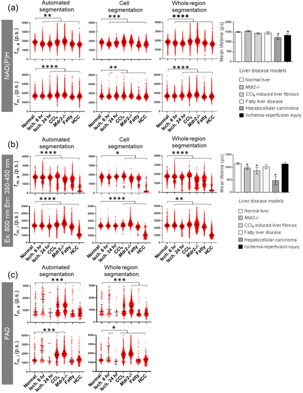
Figure 5. Amplitude weighted (τm,a) and intensity weighted (τm,i) mean fluorescence lifetime for each segmentation method for various liver conditions. (a) NAD(P)H λex 740 nm, λem 350–450 nm. (b) λex 800 nm, λem 350–450 nm channel. (c) FAD λex 800 nm, λem 515–650 nm. Median ± interquartile ranges (* p < 0.05, ** p < 0.01, *** p < 0.001, **** p < 0.0001) for all pixels from segmented analysed area (>100 photons per pixel) represented as red dots. Mean lifetime data reprinted with permission from Wang et al. [9] © The Optical Society.
Download figure:
Standard image High-resolution imageOur results also shows that the choice of segmentation method yielded similar estimates for both the NAD(P)H τm,a and NAD(P)H τm,i of all models (figure 5(a)). The similarity in the results for each of the segmentation methods probably reflects the dominance of the NAD(P)H signal in the hepatic cells in determining the τm,a and τm,i values. In particular, the FLIMFit program segmentation algorithm otsu_oht produces segmentation maps that are comprised of pixels from within cells in the NAD(P)H channel as well as the pixels in between the cells, as shown in figure 1(e). It is therefore more inclusive than manual cell segmentation but similar to whole region segmentation. The overall result is then a similar mean and range in τm,a and τm,i derived (figure 5(a)). However, it is also evident τm,a values for the different liver states vary more than τm,i for the same livers for the automation segmentation analysis. It is to be noted that, in general, the τm,i for all livers and segmentation methods is much greater than the τm,a, consistent with the greater weighting τ2 has on τm,i relative to τm,a [42].
Figure 5(b) shows our corresponding MP-FLIM findings for the λex 800 nm and λem 350–450 nm channel. It is evident that the τm,a results in Mdr2-/-, fatty liver and HCC were significantly lower than in normal livers, regardless of the segmentation method. Interestingly, the τm,i results parallel those for τm,a in showing a significant decrease only in HCC livers, whereas τm,i results from Mdr2-/- mice increased relative to normal livers (figure 5(b)).
Analysis of the distinct FAD fluorescence lifetimes are shown for various segmentations. Our initial analysis of the segmented FAD channel (λex 800 nm; λem 515–650 nm) data resulted in a1 values that spanned the whole range from 0 to 1, suggesting that no confidence could be placed in the mean a1 value. We therefore only included pixels with a minimum intensity of 100 in our subsequent regressions. We found that when an intensity threshold was applied to the data, there was a significant decrease in the number of usable pixels in each image, leading to limited usable data after cell segmentation (figure 5(c)), and that the fibrotic livers had the most remaining pixels that could be analyzed. Both τm,a and τm,i increased in the CCl4 induced and Mdr2-/- fibrosis models derived using automated and whole region segmentation methods. The values obtained for FAD τm,a (mean ± stdev) were: normal liver, 1185 ± 707 ps; ischemia-reperfusion injury at 6 h, 1691 ± 819 ps; ischemia-reperfusion injury at 24 h, 1028 ± 734 ps, CCl4 induced liver fibrosis, 1155 ± 529 ps; Mdr2-/- mice livers, 1259 ± 410 ps; fatty liver disease was 1083 ± 831 ps; and HCC, 834 ± 394 ps.
NAD(P)H model individual fitted parameters
Figure 6 shows the individual parameters derived from the bi-exponential regressions of the MP-FLIM data for NAD(P)H in different liver diseases relative to control livers and for different segmentations. It is evident that the amplitude parameters a1 and a2 do not differ greatly across the normal, and liver disease models. The data in figure 6 also shows that, in general, segmentation had little effect on the relative values of the various model parameters derived.

Figure 6. Model parameters for NAD(P)H λex: 740 nm, λem: 350–450 nm, using different segmentation methods, for various liver conditions. Median ± interquartile ranges (** p < 0.01, *** p < 0.001, **** p < 0.0001) for all pixels from segmented analysed area (>100 photons per pixel) represented as red dots.
Download figure:
Standard image High-resolution imageFAD model fitted parameters
Figure 7 shows the corresponding plots for the FAD analyses. It is evident that there is low statistical power in the cell segmentation data and, whilst the median values differ, they do so with considerable variability. These findings highlight the need for optimal imaging conditions in order to collect the most meaningful FAD data. Importantly, in the whole region and automated segmentation methods, where there is much more FAD data above the threshold photon counts per pixel than in cell segmentation, there is some evidence of two broad populations of bound FAD. Figure 7 also shows that FAD the τ2 is longer in CCl4 induced and Mdr2-/- fibrosis livers than in normal livers, with the FAD τ2 ischemia-reperfusion at 6 h showing differences in the automated and whole region segmentation data.

Figure 7. Model parameters for FAD λex: 800 nm, λem: 515–620 nm, using different segmentation methods, for various liver conditions. Median ± interquartile ranges (* p < 0.05, ** p < 0.01, *** p < 0.001, **** p < 0.0001, n.s. = not significant) for all pixels from segmented analysed area (>100 photons per pixel) represented as red dots.
Download figure:
Standard image High-resolution imageMetabolic ratios
Three commonly used metabolic ratios were calculated to assess changes in the liver: (1) redox ratio; (2) NAD(P)H amplitude ratio; (3) fluorescence lifetime redox ratio (FLIRR), that could further resolve differences between normal liver and disease state livers. The redox ratio of IFAD/INAD(P)H showed a significant increase in both fibrosis models and HCC compared to normal livers irrespective of the segmentation method. Fatty liver disease was only significantly different from normal liver in the whole region segmentation and ischemia-reperfusion injury at 24 h was significantly increased for automated and whole region segmentation formats (figure 8). The NAD(P)H ratio of a1/a2NAD(P)H showed significant decreases for all disease models and all segmentation methods. The FLIRR of a2NAD(P)H/a1FAD showed significant decrease only in CCl4 and HCC compared to normal liver for automated and whole region segmentation. With cell segmentation, there was no difference for all disease models compared to normal livers.

Figure 8. Metabolic ratios: redox ratio versus NAD(P)H ratio versus FLIRR, for different liver disease models compared to normal liver. Median ± interquartile ranges (** p < 0.01, **** p < 0.0001, n.s. = not significant) for all pixels from segmented analysed area (>100 photons per pixel) represented as red dots.
Download figure:
Standard image High-resolution imageInformed segmentation based on fluorescence lifetime
We used a sensitivity analysis of a τm,a based informed segmentation with a threshold photon count of 100 to quantify the spatial pixel distribution of collagen in the λex 800 nm, λem 350 to 450 nm channel. Figure 9(a) shows the λex 800 nm, λem 350 to 450 nm channel intensity images for our control liver and those for CCl4, Mdr2-/-, fatty liver disease and HCC. Limiting τm,a to <2000 ps and photon count >100 resulted the loss of nuclei and cell boundaries (figure 9(b)) relative to figure 9(a). A further reduction in τm,a to <700 ps, with intensity >100 photons per pixel (figure 9(c)) led to the loss of almost all pixels from normal liver cells and the retention of pixels in regions that morphologically appeared to be collagen in the fibrosed liver (figure 9(a)).

Figure 9. Informed signal segmentation assuming that pixels containing collagen are associated with short τm,a arising from a dominant effect of the negligible τm,a for the SHG of collagen. (a) Fluorescence intensity images for normal liver, fibrosis models and HCC in the λex: 800 nm, λem: 350–450 nm channel. (b) Segmented images for this channel based on τm,a < 2000 ps and intensity >100 photons per pixel. (c) Segmented images with τm,a < 700 ps and intensity >100 photons per pixel. (d) Manually drawn regions of high and low fibrosis using the images with a high pixel density in (c) (assumed to be related to a high collagen content) (red) and a second region with a low pixel density in (c) to represent the most normal region in the liver (blue). For the normal liver, 2 representative regions were chosen. (e) These same regions were then applied to the NAD(P)H data measured using λex: 740 nm, λem: 350–450 nm. Scale bar = 40 μm. Images in (a) reprinted and in (b) to (e) adapted with permission from Wang et al. [9] © The Optical Society. (f) NAD(P)H τm, a, and (g) NAD(P)H ratio for diseases that contain a collagen signal. Median ± interquartile ranges (*** p < 0.001) for all pixels from the fibrotic segmented area represented as red dots and pixels from the normal segmented area represented as blue dots (>100 photons per pixel).
Download figure:
Standard image High-resolution image
We then tested the hypothesis that these areas of fibrosis may be associated with cellular metabolic dysfunction by manual segmentation, in which we then arbitarily drew two areas of similar sizes corresponding to a fibrotic region (based on high collagen content) and a corresponding normal region (based on low collagen content), in the channel λex 800 nm, λem 350 to 450 nm (figure 9(d)) and compared the NAD(P)H signals for the two regions from images at λex 740 nm, λem 350 to 450 nm (figure 9(e)). We also included two regions of similar size from control livers for reference. NAD(P)H τm,a and NAD(P)H a1/a2 NAD(P)H ratio showed significant differences in the fibrotic region when compared to the control region (figures 9(f) and (g)). NAD(P)H τm,a increased and a1/a2 NAD(P)H ratio decreased in collagen rich areas in both CCl4 and Mdr2-/- fibrosis models, whereas HCC showed the opposite results. Surprisingly, fatty liver disease did not show any difference in NAD(P)H τm,a and a1/a2 NAD(P)H ratio.
Discussion
Technically challenging intravital MP-FLIM imaging has been performed on liver, skin, brain, and kidney to detect endogenous fluorophores and achieve analysis of metabolic cofactors NAD(P)H and FAD [9, 36, 45–50]. To date, most studies define NAD(P)H free as being in the cytoplasm and NAD(P)H bound being in the mitochondria and are associated with glycolysis and oxidative phosphorylation in the two sites, respectively. Remarkably, NADH and NADPH are involved in 488 human metabolic reactions which are not confined to the mitochondria for energy production, but are also located in the cytosol and nucleus in processes as wide ranging as transcriptional regulation and DNA repair [25]. Therefore, our understanding and interpretation of NAD(P)H and FAD MP-FLIM images are still developing. Importantly, alterations in the fluorescent lifetime of NAD(P)H free and FAD bound may not only reflect a shift in metabolic pathway but could also reflect either a change in lipid and protein synthesis and/or microenvironment changes, including variations in pH, concentration of oxygen, tyrosine, or tryptophan. Accordingly, limiting MP-FLIM analysis to the most commonly reported single metric of τm,a for NAD(P)H and optical redox ratio will provide only a limited understanding of how liver injury and liver disease has affected the redox state of the liver. Increasingly, both NAD(P)H free and bound metrics, including τ1 and τ2, along with multi-parametric analysis is likely to become more important [46, 51].
In order to examine the impact of the heterogeneity in the in vivo liver cells and spaces as a result of liver disease, this work has undertaken a more complete analysis of MP-FLIM data from normal and liver disease models than we have ever undertaken previously. In particular, this work has explored the impact of segmentation and disease state on the bi-exponential FLIM parameters for the endogenous fluorophores NAD(P)H and FAD, as well as in the λex 800 nm, λem 350 to 450 nm channel, and the various metabolic ratios that can be derived from these parameters. The work extends our previous work in vivo which reported the most common metric for FLIM, the τm,a for NAD(P)H in hepatocytes [9]. The previous work showed the τm,a of NAD(P)H in normal liver (mean, stdev) was 1.511 ± 0.032 ns was estimated using λex 740 nm λem 350 to 450 nm. Our FAD analysis was limited by our previous FLIM data being collected at λex 800 nm and λem 515–650 nm [9]. Figure 1(d) shows that the more commonly used λex 740 nm and λex 890 nm avoid the small bleed through effect that may be seen from NAD(P)H in FAD estimation. The use of λex 890 nm for FAD estimation may also be desirable in liver fibrosis to avoid overlapping fluorescence from elastin (2P λex of 760 to 830 nm, an emission λem 475 to 575 nm and short and long lifetimes of 260 and 1960 ps [42]) that is often associated with liver fibrosis. Recently, Cao et al used a single λex of 800 nm to imaging both NAD(P)H and FAD with emission filters of λem 450/50 nm and 560/80 nm, respectively, indicating this method may be preferred in vivo to decrease total imaging time, to avoid motion artifacts and increase temporal resolution, as needed in clinical settings [41].
Collagen emission is a second harmonic generated process with an effectively instantaneous fluorescence lifetime. With data collected at λex 800 nm, λem 350 to 450 nm channel, we found a τm,a of about 1700 ps (figure 5(b)) reports of collagens (I, II and III) having τm,a of around 1.5 ns [52] or 0.29 ns and 1.68 ns at λex 830 nm [53]. Visualized pixels with τm,a < 2000 ps (figure 9) did not have morphology consistent with that anticipated for collagen. The apparent loss of nuclear and cell membrane structures in images for 700 < τm,a < 2000 ps (figure 9) suggest that cellular components contribute to the apparent τm,a of ∼1700 ps shown in figure 5(b). We have shown elsewhere, using phasor analysis, that the τm,a for collagen in diseased livers is 87 ps [54] and the segmented images with τm,a < 700 ps appeared to have collagen like morphology. Further, it is evident that increased collagenization in fibrotic livers (figure 9) corresponds with an overall decrease in the τm,a for those same livers in the λex 800 nm, λem 350 to 450 nm channel (figure 5(b)), consistent with the dominant effect of the essentially instantaneous collagen signal on the overall lifetimes.
In this report, we re-examined aspects of the data processing with different segmentation techniques and determined optimal parameter estimates of the fitted data to the heterogeneous datasets produced by different liver diseases. Multiple protocols used to obtain quality FLIM data [55–58], have mentioned the importance of calibration of the system, using fluorescein or rhodamine to estimate the correct IRF for model fitting and image analysis, and methods have been developed to estimate the correct IRF from reference images [59–61]. The most emphasised consideration of time-correlated single photon counting is the minimum amount of photons necessary for robust data fitting, which is generally 1000 photons per pixel and when not met, can lead to artefacts in the results [58]. We and others have been able to produce reliable model fitting to as low as 100 photon counts per pixel [62]. Many publications have shown that binning of data increases the confidence of model fitting without significantly change changing to the estimated parameters [35, 63, 64]. However, others have noted that, in heterogeneous samples such as diseased livers or the retina of the eye [65], binning can result in erroneous fluorescence lifetimes [66]. Lastly, the effect of segmentation was explored and we found that with fine segmentation of cytoplasm compared to nucleus compared to liver sinuses, we were able to detect differences in the NAD(P)H ratio of a1/a2NAD(P)H. However, when we compared segmentation of automated segmentation to a whole region centered in the image in FLIMFit, τm,a, τm,i, a1, a2, τ1 and τ2 did not vary significantly between segmentation methods for NAD(P)H and FAD. However, small differences could be discerned in τm,a and τm,i for the (figure 5(b)). The location of the NAD(P)H binding signal has always thought to be in the mitochondria, and that of free signal to come from the cytoplasm. However, one study using a higher single cell resolution, reduced binning and a pixel-wise two exponential fit has demonstrated that distinct NAD(P)H bound fluorescent lifetimes in adipocytes arise from the mitochondria as well as the cytoplasm [35]. This has led to the suggestion that the two short lifetimes seen in adipocytes represent folded (0.4 ns) and extended (0.9 ns) conformations of free NAD(P)H in solution whereas the two longer lifetimes represent two different binding states. It was further suggested that the ratio of free to bound NAD(P)H defines a glycolysis/oxidative phosphorylation ratio and a change in ratio reflects a change in enzyme binding [35]. Similarly, the evaluation of metabolic ratios using a higher resolution FLIM imaging of NAD(P)H, FAD and Trp found heterogeneity within the cells [67].
Importantly, Wallrabe et al [67], in measuring FLIM parameters for NAD(P)H, FAD and tryptophan in segmented, thresholded, xenograft cancer cell, reported that light-scattering and laser power needs in tissue sections made the FAD/NAD(P)H photon ratio (an intensity-based redox measurement) unsuitable for tissue sections. They suggested that the segmented, threshold, ROI approach using many data points to visualise differences between and within cells, as we have also described here, is preferred to the usual means based analyses. They also reported a heterogeneity and increase in FLIRR cellular responses after glucose stimulation. This simulates the aerobic glycolysis or Warburg effect seen in many tumor cells. However, high energy utilisation at the tumor edge of in vivo solid tumors may be accompanied by a hypoxic core, which may eventually become necrotic as a consequence. The stage and heterogeneity of the solid tumor will give rise to opposing FLIRR values dependent on the imaging site within the tumor.
We explored several combinations of NAD(P)H and FAD measured FLIM parameters based on theory developed in the field to capture the metabolic changes within cells in the liver during different disease states. In our analysis, we found that fibrosis, either in CCl4 induced fibrotic hepatocytes or Mdr2-/- fibrotic biliary cells, could be distinguished by an increase in the redox ratio. Indeed, Mdr2-/- fibrosis is distinguishable through all 3 metabolic ratios assessed, irrespective of segmentation strategy used as there is an increase in the redox ratio, a decrease in the NAD(P)H ratio and an increase in FLIRR when compared to normal liver. These changes are due to an increase in τ1 in both NAD(P)H and FAD indicating there are multiple metabolic pathways involved in this pathogenesis which modulate both NAD(P)H and FAD. In particular, a combined significant increase in redox ratio and decrease in τm,a for the the λex 800 nm, λem 350 to 450 nm channel is a potential MP-FLIM predictor for HCC that may be useful in its diagnosis. In the ischemia-reperfusion injury model used here the bile duct was not clamped. In contrast, in other studies in which the portal vein, hepatic artery, and bile duct were clamped [2], there was an increase in FAD intensity and a decrease in NAD(P)H intensity [33] that could further distinguish a liver ischemia-reperfusion injury from other liver diseases.
Two other studies relevant to our analysis presented multi-parametric results to stratify metabolic response. In one case, an indicator of the metabolic responsiveness of the breast cancer to drug therapy over time and was based on an index that was the linear combination of three normalized parameters: redox ratio, NAD(P)H τm,a and FAD τm,a [68]. This approach tracks the metabolic changes over time and contrasts to the cross-sectional time data described here for different liver conditions. In another study, cells were subjected to hypoxia and glucose starvation, mitochondrial uncoupling, and fatty acid oxidation while 3 parameters: redox ratio, the NAD(P)H fluorescence lifetime, and mitochondrial clustering were used to distinguish distinct metabolic states in multiple cell types in vitro and in vivo [46]. This work parallels our goal to provide a combination of FLIM parameters that can provide a distinguishing signature for different liver injury and disease states for use as a diagnostic tool.
Recently, the validity of metabolic ratios reported in the literature from in vitro and in vivo studies has been questioned. In particular, the metabolic index NAD(P)+/NAD(P)H ratio has been challenged as a result of the assumed lifetime values for free and bound NAD(P)H, and differences in the NAD(P)H bound lifetimes reported from studies analyzing FLIM data with two, three, or four exponential fits versus the phasor approach [69]. Different FLIM acquisition hardware, acquisition considerations, as well as data analyses that can affect the reported NAD(P)H bound have been highlighted. For example, whether a full fluorescence decay is captured in the acquisition time window will affect the fitting, or whether the model fitting was applied globally or pixel-wise will ultimately affect the reported NAD(P)H bound lifetime. In line with this, we showed that variation in the data occur with the choice of programs to calculate the fit, when different IRF are applied and is dependent on the binning that is applied to the data. Efforts to validate the FLIM of NAD(P)H and FAD has been ongoing for many years. Studies have tried to separate NADH and NADPH using FLIM analysis to determine the relative contribution [29]. Indirect measurements using mass spectroscopy has shown that the expression of NAD and/or NADP differs between various tissues [70–72]. A normalized optical redox ratio FAD/(NAD(P)H + FAD) has also been used to measure the cell redox changes associated with stem cell differentiation and the optical redox ratio was correlated to the gold-standard liquid chromatography/tandem mass spectrometry (LC/MS) measurements of intracellular cofactor concentrations. Surprisingly, the optical redox ratio FAD/(NAD(P)H + FAD) correlated to the LC/MS measurements of NAD(P)+/(NAD(P)H + NAD(P)+) but did not correlate to the LC/MS measurements of FAD/(NAD(P)H + FAD) [73]. The optical redox ratio has also been shown to correlate well to the rate of oxygen consumption measurements made on the metabolic analyzer (Seahorse XFe24, Seahorse Bioscience) when ETC disruptors were applied [74]. An in vivo FLIM study of the brain systematically applied metabolic inhibitors to the brain surface under a cranial window to discern differences in NAD(P)H during metabolic perturbation to glycolysis, the TCA cycle, the ETC, or oxidative phosphorylation [36]. A careful analysis of multiple NAD(P)H FLIM parameters was used to detect differences between the aforementioned metabolic states.
We have shown that MP-FLIM is a sensitive and useful method to interrogate changes in metabolism and that segmentation based on other structural or functional markers such as collagen could aid in identifying distinct cellular subpopulations. This work is relevant to recent single cell RNAseq studies showing liver cell populations can be stratified into many functional subsets [75, 76]. This work has also used Becker & Hickl TCSPC data recording on a Dermainspect MPM in our in vivo real time clinical imaging approach. Others have proposed a wide-field, time-gated FLIM approach based on only four images, with high precision being achieved by either a summing of frames or by use of pixel-binning [77]. However, our work here has shown that spatial resolution may be compromised by pixel binning, leading to erroneous results in heterogeneous samples and the summing of frames may also need to be corrected for intravital motion [10].
Acknowledgments
The authors have declared that no conflicting interests exist. This work was supported by grants from the National Health and Medical Research Council of Australia (Grants: 1049906; 1049979, 1002611, 1126091, 1107356). Many thanks to Leslie Burke for a careful review of the manuscript. The authors from the Diamantina Institute are based at the Translational Research Institute (TRI), Queensland, Australia.
We thank Dr Svetlana Rodimova, a researcher at the Privolzhsky Research Medical University, Russia, who inspired much of this paper through her request for us to expand on our 2015 Real-time Histology in Liver Disease paper [9] by publishing the relative contributions of a1 and a2 for NAD(P)H and the fluorescence life-time data for FAD, for comparison with their work [33, 34], and who also reviewed this paper. We also implicitly acknowledge Dr Sean Warren, the author of FLIMFit software tool developed at Imperial College London that was used for the analysis of most of the images described here. We also express our appreciation to Dr Wolfgang Becker, the developer of the TCSPC technology used in the FLIM analysis and of SPCImage5.5 that was used to collect the TCSPC data for individual images. Lastly, we are grateful to Drs Hauke Studier and Wolfgang Becker of Becker & Hickl Pty Ltd for providing us with an evaluation copy of SPCImage 8 for use in this work.