


ABSTRACT
We found that a surge consists of multiple shock features. In our high-spatiotemporal spectroscopic observation of the surge, each shock is identified with the sudden appearance of an absorption feature at the blue wings of the Ca ii 8542 Å line and Hα line that gradually shifts to the red wings. The shock features overlap with one another with the time interval of 110 s, which is much shorter than the duration of each shock feature, 300–400 s. This finding suggests that the multiple shocks might not have originated from a train of sinusoidal waves generated by oscillations and flows in the photosphere. As we found the signature of the magnetic flux cancelations at the base of the surge, we conclude that the multiple shock waves in charge of the surge were generated by the magnetic reconnection that occurred in the low atmosphere in association with the flux cancelation.
Export citation and abstract BibTeX RIS
1. INTRODUCTION
Surges are the violent ejections of cool and dense plasma in the solar chromosphere, mostly in active regions. They are ejected with the speed exceeding several tens of km s-1 along either a straight trajectory or a slightly curved one. They reach up to 10,000–100,000 km, and then fall down along the same trajectory (Tandberg-Hanssen 1995).
Previous observations produced results supporting that surges are related to magnetic reconnection occurring in the atmosphere. Roy (1973) first found that surges tend to grow from small bright knots, either Ellerman bombs (EBs) or subflares. It was also found that the surges occur in regions of parasitic satellite polarity or evolving magnetic features, which provides a magnetic environment suited for magnetic reconnection. The subsequent observational studies of EBs have supported the low-atmosphere reconnection origin of EBs (e.g., Dara et al. 1997; Georgoulis et al. 2002; Watanabe et al. 2011). The recent case study of an EB and its associated features—velocity field and magnetic field in the photosphere, the motion of the EB, and the motion and temperature of its associated surge (Yang et al. 2013) produced detailed results quite compatible with this idea. Meanwhile, Canfield et al. (1996) found that many surges occur at places adjacent to X-ray jets and suggested that X-ray jets represent hot plasma jets coming out of magnetic reconnection while surges are cool plasma jets driven by the slingshot process as seen in the simulation of Yokoyama & Shibata (1996). A similar relationship was later found among EUV jets—a miniature of X-ray jets, small surges, and emergence and subsequent cancelation of magnetic flux (Chae et al. 1999), which also supports the magnetic reconnection origin of surges.
Very recently, Takasao et al. (2013) found from numerical simulations that slow shock waves generated by magnetic reconnection in the chromosphere and the photosphere play key roles in the acceleration mechanisms of chromospheric jets. The idea of a slow shock-wave-driven surge itself was first proposed by Shibata et al. (1982), who found from hydrodynamic simulations that sudden pressure increase at a low height generates shock waves that produce jets. Takasao et al. (2013) demonstrated that magnetic reconnection taking place near the photosphere can generate slow waves that move upward along magnetic field lines and develop into slow shock waves. This idea of reconnection-generated shock waves as the driver of surges is very interesting, but has not yet been observationally verified. In this Letter, we present observational evidence for this idea for the first time. Specifically, we report the unexpected existence of multiple shock features comprising the surges. Our result supports the idea that the energy released by the magnetic reconnection in the low atmosphere is transported upward in the form of the shock waves and drives the surges.
2. OBSERVATION
We focus on the Doppler velocity variation in a series of recurring surges. The data were obtained using the Fast Imaging Solar Spectrograph (FISS) and the TiO broadband filter installed at the 1.6 m New Solar Telescope (NST) at the Big Bear Solar Observatory. The FISS is an Echelle spectrograph that provides spatial and spectral information of the two lines, Hα and Ca ii 8542 Å, simultaneously. As the adaptive optics of the NST was recently upgraded from the 76 segment system to the 308 segment system, FISS has provided unprecedented imaging-spectrographic data with high temporal resolution. One can find detailed information on the instrument from Chae et al. (2013). Basic image processing of the FISS data, such as flat-fielding, dark subtraction, and distortion correction, was carried out using the methods described in Chae et al. (2013) and the wavelength calibration was done following Yang et al. (2013). The rotation and alignment of the data were also corrected.
On 2013 August 16, our observation was performed with the field of view (FOV) of 19 2 × 40'' in steps of 20 s for 80 minutes from 19:41:11 UT to 20:56:06 UT (hereafter the time 19:41:11 UT is taken as the epoch of time t) using FISS. The step size in the scan was set to 016 which is equal to the sampling interval along the slit. There are some missing data due to the temporary failure of the adaptive optics.
The TiO filter was centered at a wavelength of 7057 Å with 10 Å band width (Cao et al. 2010). Each burst consisting of 70 TiO images was taken in 15 s with exposure time of 0.8 ms. The data were dark subtracted, flat-fielded, and then applied the Kiepenheuer-Institut Speckle Interferometry Package (Wöger et al. 2008) code to each burst. The FOV of the speckle-reconstructed images was 698 × 698.
A series of surges were repeatedly ejected from its base located at (226'', −207'') southward, following the same curved trajectory. Two surges of projected sizes >10'' occurred during the observation, one during the time interval 300 s–1100 s (hereafter surge i) and another during the time interval 1760 s–3542 s (hereafter surge ii). The other smaller surges occurred between these two surges. Figure 1 shows the temporal evolution of surge i. It was first visible in absorption at about t = 300 s at the blue wings of the Hα and Ca ii 8542 Å lines. After that, the absorption feature gradually moved toward the red wings in both the spectral lines.
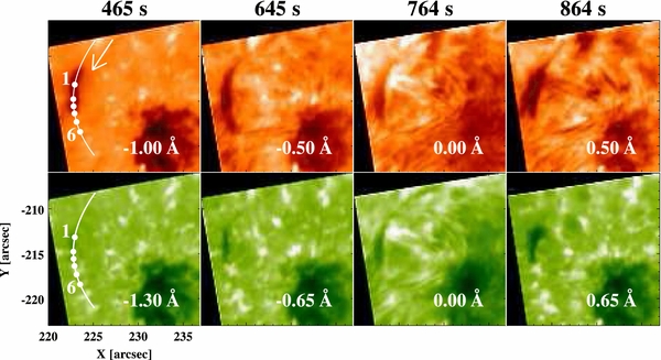
Figure 1. Temporal evolution of surge i at the blue wings and red wings of the Hα (top) and Ca ii 8542 Å (bottom) lines. The white dots and the curve indicate the selected positions for analysis in Figures 2 and 3. The white arrow represents the direction of the surge ejection.
Download figure:
Standard image High-resolution imageIn order to clearly show the spatial behavior of the absorption features, we made a contrast profile Cλ, which is defined as Cλ = (Iobs − Iref)/Iref. Figures 2 and 3 are drawn with the contrast profiles. We identified Iref with the averaged profiles of about 180 profiles obtained at the same position during the observation.

Figure 2. Wavelength–time plots in Ca ii 8542 Å (leftmost six plots) and Hα (rightmost three plots) lines at six spatial positions marked by the white dots in Figure 1. The numbers in parentheses represent the distance from the brightening positions in the SDO/AIA 1600 Å images. Two big surges appeared during the time interval of 300–1100 s and 1760–3542 s. The white dots are the positions where the largest amplitude shock features were first shown in each plot.
Download figure:
Standard image High-resolution image
Figure 3. Wavelength–distance plots at different times (titles in the individual plots) in Ca ii 8542 Å (leftmost six plots) and Hα (rightmost three plots) lines. The distance was measured from the brightening positions in the SDO/AIA 1600 Å images (see Figure 5) along the white curve marked in Figure 1. The white arrow represents the direction of the surge ejection, as the same with the direction of the arrow in Figure 1. The white dotted lines represent that the diagonal components show at the blue wings first, then stretched and redshifted with time.
Download figure:
Standard image High-resolution image3. RESULT
The most striking result is that a surge appears as a group of diagonal dark components in the Ca ii wavelength–time (λ–t) plots in Figure 2. We computed the λ–t plots from six spatial positions marked by the white dots in Figure 1. In the Ca ii λ–t plots, surge i is identified as the group of four to five diagonal dark components (white dotted lines on the third panel in Figure 2), and surge ii also consists of more than three diagonal dark components. In the lower part of the surge i (panels (1)–(3) in Figure 2), each component suddenly appeared with the large blueshift of about 70 km s-1, and then the speed decreased with an deceleration of about 0.19 km s-2. In the upper part of the surge i (panels (4)–(6) in Figure 2), it appeared with the blueshift of about 20 km s-1 and a deceleration of about 0.29 km s-2.
What is important is that a surge is resolved into several dark components that successively occurred with the 110 s time interval, which is much shorter than the duration of each feature, 300–400 s. These overlapped features were found in the lower part of the surge, but only one or two diagonal components remained in the upper part. Interestingly, the amplitude of the first diagonal components was smaller than the amplitude of the next one in the surge.
Note that the overlapped diagonal dark components differ from the recurrence of surges. The recurrence is the repeated occurrence of individual surge ejections at the same location at different times. However, these components coexist at the same time in each surge. The overlapped features are not resolvable in the Hα λ–t plots (rightmost three panels in Figure 2) because the Doppler width of the Hα is so broad that the features are smeared out.
The dark diagonal components are also identified in the Ca ii wavelength–distance (λ–dist) plots of Figure 3. Each diagonal component appeared at the blue wings of the contrast spectral profiles. The trailing part of each component is redshifted compared to the front part. Every diagonal component stretched upward (white dotted lines in Figure 3). When the features reached the peak height, it started falling down as absorption at the red wings. This spatiotemporal pattern of Doppler shift is similar to that of the early study of Tamenaga et al. (1973) as presented in their Figure 6.
In Figures 2 and 3, each diagonal component suddenly appeared with large blueshift followed by the gradual drift to large redshift. This discontinuity of the physical quantities in space and time is the typical characteristic of a shock wave (Kalkofen et al. 2010). In this regard, we suppose that each diagonal component represents the shocked gas behind a shock front. The shock waves may be generated at the base of the surge and propagate into the corona.
Figure 4(a) shows the variation of the line-of-sight (LOS) speed of the shocked gas at the front over distance. The speed and distance of the front at each instant is marked by a white dot in Figure 2. The figure shows that the shocks first appeared with the speed of about 70 km s-1in the low atmosphere. This is much faster than the sound speed of the order of 10 km s-1 in the chromosphere, suggesting a high value of the initial Mach number >7. The speed of the front then significantly decreased with distance, becoming as low as 20 km s-1, which indicates that the shock got weakened much as it propagated. Figure 4(b) shows the arrival time of the same front as a function of distance. The slope of the straight line fit means the inverse of the projected propagation speed of the shock, which is found to be about 17 km s-1. This speed is much lower than the initial LOS speeds of the front shown in Figure 4(a), implying that only a small portion of the full propagation velocity may have been projected onto the plane of the sky and hence the direction of the surge may be highly inclined to the line of sight.

Figure 4. (a) Spatial evolution of the LOS speed of the shocked gas and (b) the temporal evolution of the projected propagation of the shock front. The positive value represents the upward motion.
Download figure:
Standard image High-resolution imageWe found magnetic flux canceling features and brightening events at the base of the surge. The LOS magnetogram (in Figure 5) taken by the Helioseismic and Magnetic Imager (HMI; Schou et al. 2012) of the Solar Dynamic Observatory (SDO) reveals the parasitic magnetic element of positive polarity located at the base of the surge. It emerged at a region about 3'' south from the base and approached it. After that it canceled with its surrounding negative polarities. Two photospheric elongated granule-like features, which may be regarded as the indication of small-scale flux emergence (Lim et al. 2011; Yang et al. 2013), were seen in the TiO images as shown in Figure 5(c). They reached the base of the surges just before the ejections of the corresponding surges. It emerged and moved together with the parasitic positive polarity. The UV images at 1600 Å and 1700 Å taken by the Atmospheric Imaging Assembly (AIA; Lemen et al. 2012) of SDO display brightening events on the edge of the parasitic polarity. They took place simultaneously with the ejections of surges at the base of them. They last longer until the surges fell back. In addition, flare-like EUV brightenings occurred for short time in the SDO/AIA 304 Å images at the same place as the highly blueshifted features of the surge ii at 1700 s and 2000 s. We also found a mustache-shaped spectra of the Hα line, that is typical shape of the EB spectra, at the base of the surges. These results indicate that an abrupt energy release in the low atmosphere like magnetic reconnection may be responsible for the surges.

Figure 5. (a) FISS Hα-1 Å raster image taken at t = 485 s, (b) the SDO/AIA 1600 Å filter image at t = 473 s, and (c) the TiO filter image at t = 105 s. The contours represent the LOS magnetic field in the SDO/HMI magnetogram. The white arrow in panel (c) points to the elongated granule-like feature.
Download figure:
Standard image High-resolution image
4. DISCUSSION
We found multiple shock features in the surges that have not been discovered earlier. These kind of features cannot be observed without high spectral resolution and high temporal resolution. Note that the Doppler width of the Hα line is too broad for these features to be spectrally resolved. We also found the observational signatures of magnetic reconnection at the base of the surge. These findings suggest that the shock waves generated by the energy release through magnetic reconnection in the low atmosphere propagate into the chromosphere and appear as surges.
It is well known that the compressional waves steepen to form shocks in a gravitationally stratified medium like the solar chromosphere (Carlsson & Stein 1997). For instance, dynamic fibrils (DFs) are considered to be shock waves with an interval of three minutes that originate from the photosphere and propagate along inclined field lines (De Pontieu et al. 2007; Langangen et al. 2008), and three minute oscillations in the chromosphere are found to be the LOS velocity variations of the saw-tooth shape, or N-shape, which represent the shock waves. These shock waves are most likely to be developed from the waves originating from the photospheric oscillation. In contrast, surges seem to be driven by the shock waves produced by the abrupt energy release, such as magnetic reconnections, occurring in the low atmosphere. The slow mode waves may easily develop into shocks, and then the shocks propagate along the field lines. Our finding of the shock patterns inside the surge is in good agreement with the simulation results of Shibata et al. (2007) and Takasao et al. (2013).
The shocks comprising the surges differ from the shocks of the DFs or the chromospheric oscillations in the way how multiple shocks arrive. In the latter case, the time interval between the consecutive shocks is about 3 minutes, which is the same as the duration of each shock. This means that the shocks develop from a single train of sinusoidal waves. In the surge, however, the time interval is 110 s, that is, shorter than the duration time of each shock 300–400 s. Thus, it is not likely that the multiple shock waves we observed originate from the single train of sinusoidal waves unlike the case of DFs. If that is the case, how should we understand the train of shocks with 110 s time interval? One possibility is that we may be simultaneously observing several slow mode shocks originating from the same source, but propagating along different magnetic flux tubes at different phases. The numerical simulations indicated that the fast mode shocks generated in the outflow region of the magnetic reconnection can be converted to the slow mode waves along the multiple flux tubes (Yokoyama & Shibata 1996; Takasao et al. 2013). Another plausible scenario is that the multiple shocks of short time interval may be due to multiple magnetic reconnection or multiple plasmoid ejections in the reconnection site (Nishizuka & Shibata 2013). In any case, it seems to be the fine-scale structure of magnetic field and magnetic reconnection in the low atmosphere that are responsible for the observed multi shock structures of the surges.
We appreciate the referee's constructive comments. This work was supported by the National Research Foundation of Korea (NRF-2012R1A2A1A03670387). E.-K. Lim is supported by the "Study of near-Earth effects by CME/HSS"project and basic research funding from KASI.