


ABSTRACT
Since the last Pluto volatile transport models were published in 1996, we have (1) new stellar occultation data from 2002 and 2006–2012 that show roughly twice the pressure as the first definitive occultation from 1988, (2) new information about the surface properties of Pluto, (3) a spacecraft due to arrive at Pluto in 2015, and (4) a new volatile transport model that is rapid enough to allow a large parameter-space search. Such a parameter-space search coarsely constrained by occultation results reveals three broad solutions: a high-thermal inertia, large volatile inventory solution with permanent northern volatiles (PNVs; using the rotational north pole convention); a lower thermal-inertia, smaller volatile inventory solution with exchanges of volatiles between hemispheres and a pressure plateau beyond 2015 (exchange with pressure plateau, EPP); and solutions with still smaller volatile inventories, with exchanges of volatiles between hemispheres and an early collapse of the atmosphere prior to 2015 (exchange with early collapse, EEC). PNV and EPP are favored by stellar occultation data, but EEC cannot yet be definitively ruled out without more atmospheric modeling or additional occultation observations and analysis.
Export citation and abstract BibTeX RIS
1. INTRODUCTION
Because Pluto's predominately N2 atmosphere is in vapor-pressure equilibrium with the solid N2 ice on its surface, the surface pressure is a sensitive function of the N2 ice temperature. Furthermore, volatiles migrate from areas of higher insolation to areas of lower insolation, carrying both mass and latent heat (Stern et al. 1988; Spencer et al. 1997). Pluto's changing heliocentric distance and subsolar latitude leads to complex changes in Pluto's volatile distribution and surface pressure over its season. The first realistic models of Pluto's seasonal change were constructed in the mid-1990s (Hansen & Paige 1996, hereafter HP96), postdating the definitive discovery of Pluto's atmosphere (Hubbard et al. 1988; Elliot et al. 1989), the identification of N2 as the dominant volatile on the surface and in the atmosphere (Owen et al. 1993), and maps of the sub-Charon face of Pluto from mutual events (Buie et al. 1992; Young & Binzel 1993). Most simulations in HP96 predicted large changes in Pluto's atmospheric pressure on decadal timescales.
New observational constraints postdating HP96 include occultations in 2002 and 2006–2012 (e.g., Elliot et al. 2003a; Sicardy et al. 2003; Young et al. 2008a; see Table 2), global albedo maps from Hubble Space Telescope (HST) observations in 1994 and 2002–2003 (Stern et al. 1997; Buie et al. 2010b), schematic composition maps based on visible HST maps and visible and near-IR spectra (Grundy & Fink 1996; Grundy & Buie 2001), and rotationally resolved thermal emission (Lellouch et al. 2000, 2011).
NASA's New Horizons spacecraft will fly by the Pluto system in 2015 July (Stern 2008). Much of the planning is based on the expectation, from HP96 models and occultation observations, that the atmosphere now through encounter is in a slowly changing pressure plateau. However, models and computers from the mid-1990s limited the number of cases that could be investigated by HP96. If the pressure plateau ends near or before 2015, this will have profound implications for the world that New Horizons will encounter, and our ability to relate this snapshot to preceding or following observations. Volatile transport models can also guide how observations of Pluto's surface albedo, composition, and temperature, and its atmospheric structure and composition, can provide a temporal context for the flyby. For this reason, we have developed new volatile transport models with application to Pluto (Young 2012; L. A. Young, in preparation), and qualitatively compared simulations to occultation, visible, thermal, and near-infrared data.
2. VOLATILE TRANSPORT MODEL
This study uses the three-dimensional volatile-transport (VT3D) code developed in Young (2012) and L. A. Young (in preparation). As in HP96, energy is balanced locally between (1) insolation, (2) thermal emission, (3) conduction, (4) internal heat flux, and, in areas covered by solid N2, (5) latent heat of sublimation, and (6) specific heat needed to raise the temperature of the volatile slab. The internal heat flux is taken to be 6 erg cm−2 s−1, following HP96. The latent heat of crystallization of the N2 phase change at 32.6 K has a minor effect on the seasonal variation of Pluto or Triton (Spencer & Moore 1992) and is ignored in this Letter. The main advantages of VT3D for a parameter-space search of Pluto's seasonal volatile transport is rapid calculation based on an efficient matrix formulation, and an initial condition that decreases the time to reach convergence.
For current-day Pluto, and for much of Pluto's orbit, Pluto's atmosphere effectively transports both mass and energy (in the form of latent heat) from areas of high to low insolation (Stern et al. 1988; Spencer et al. 1997). In this "global atmosphere" regime, the volatile ice temperature is nearly uniform over the entire body, as is the surface pressure. Conservation of mass, integrated over the entire body, is used to eliminate the latent-heat terms in the energy equations (Young 2012). When Pluto's atmosphere is too tenuous to maintain an isothermal, isobaric surface, VT3D treats the surface as a splice between areas with efficient transport, which share a common volatile ice temperature and surface pressure, and areas with no lateral transport of volatiles, where ice temperatures follow strictly local energy balance.
Because Pluto's ice temperature should vary only minimally over a Pluto day (Young 2012), this Letter averages solar insolation over latitude bands. Simulations were initialized at aphelion, with the specified N2 inventory distributed evenly over the surface. Results starting at other times in the orbit are qualitatively similar. Surface and subsurface temperatures were initialized using a sinusoidal decomposition of solar forcing, as described in Young (2012) and L. A. Young (in preparation), which dramatically improved convergence.
Temperatures within the substrate were calculated at 2.5 points per seasonal skin depth, down to 7.2 skin depths. Temperatures were calculated with 240 timesteps per Pluto year, or just over 12 Earth months per timestep. With this timestep, the explicit forward-timestep is stable and was used in the calculations presented here. Only three Pluto years were needed before the simulations converged (that is, the N2 ice temperatures in the second and third years differed by only a few percent of the peak-to-peak seasonal variation).
3. PARAMETER SPACE SEARCH
Calculation of a single Pluto simulation is very fast, allowing a wide parameter space search. The bolometric hemispheric albedo, AV, of the N2 ice was varied from 0.2 to 0.8 in steps of 0.2. This range matches the range of values used by HP96 and includes the values described as good or acceptable fits by Lellouch et al. (2011, hereafter L11). The emissivity of the N2 ice, εV, was calculated at only two values, 0.55 and 0.8. The lower value was adopted by Young (2012), based on L11, while 0.8 emissivity is the highest considered by HP96. The substrate bolometric hemispheric albedo, AS, was fixed at 0.2 for all runs, based on the rough agreement of runs 12, 34, and 38 of HP96 with the occultation record and the Tholin/H2O albedos used by L11. Results are not sensitive to changes in the substrate albedo, as long as it is low. All runs used a substrate bolometric emissivity, εS, of 1.0, based on the "good fits" of L11. The thermal inertia, Γ, was varied logarithmically at 2 values per decade between 1 and 3162 J m−2 s−1/2 K−1. (MKS units are used for Γ for convenience and comparison with recent literature.) This range is a superset of the values modeled by HP96 (41–2100 J m−2 s−1/2 K−1), and includes the thermal inertia derived by L11 (∼18 J m−2 s−1/2 K−1) and the thermal inertia for pure, solid, H2O (∼2100 J m−2 s−1/2 K−1; Spencer et al. 1997). The total N2 inventory,  , ranged from 2 to 64 g cm−2, varying by factors of two, a range that includes the values modeled by HP96.
All 672 simulations were passed through a coarse sieve to identify those results roughly consistent with stellar occultations in 1988 and 2006 (Elliot et al. 2003b; Young et al. 2008a; Lellouch et al. 2009), requiring that the surface pressure in 1988 is 3–52 μbar, the surface pressure in 2006 is 7–78 μbar, and the pressure in 2006 is 1.5–3.1 times higher than in 1988.
Of all the simulations, 51 matched the coarse sieve (Table 1). The volatile migration patterns for each of these runs were found to fall into one of three categories. Half had volatiles on the northern (current summer) hemisphere throughout the entire Pluto year and fall into the Permanent Northern Volatile (PNV) category (Figures 1(A) and (B)). PNV runs generally have high-thermal inertia, Γ, delaying the transfer of volatiles from the summer to the winter pole after the perihelion equinox (Figure 2(A)). All PNV runs have gradual pressure changes; about half have pressures between 10 and 100 μbar throughout the entire year, and all have minimum pressures above 0.4 μbar.

Figure 1. Results for PNV9 ((A) and (B)), EPP7 ((C) and (D), and EPC7 ((E) and (F)). For each run, the plot on the left shows Pluto over a season. The circles represent Pluto at each of 12 equally spaced times in the orbit, indicated by date. The short vertical bar behind the circles represents the rotational axis, oriented so that the axis is perpendicular to the sun vector at the equinoxes, with the northern pole at the top (currently pointed sunward). Latitude bands are colored with their geometric albedos. The plots on the right show geometric albedo and surface pressure as a function of year. Note the large change in pressure scales ((B), (D), and (F)).
Download figure:
Standard image High-resolution image
Figure 2. Parameters for (A) PNV (plus EPP1 and EPP2), (B) EPP (excepting EPP1 and EPP2), and (C) EEC categories. Circles are centered on the corresponding volatile hemispheric albedo (AV) and thermal inertia (Γ). Circle sizes relate to the total N2 inventory, ranging from 2 g cm−2 (smallest circles) to 64 g cm−2 (largest circles). Thicker circles represent the 19 preferred runs.
Download figure:
Standard image High-resolution imageTable 1. Runs that Pass the Coarse Sieve, Sorted by 2015 Pressure within Each Category
| Γ |  |
Surface Pressure (μbar) | ||||||
|---|---|---|---|---|---|---|---|---|
| Run | AV | εV | (J m−2 s−1/2 K−1) | (g cm−2) | 1988 | 2002 | 2006 | 2015 |
| PNV1 | 0.50 | 0.80 | 3162. | 16 | 36 | 63 | 75 | 102 |
| PNV2a | 0.60 | 0.55 | 3162. | 2 | 35 | 58 | 68 | 95 |
| PNV3 | 0.50 | 0.80 | 3162. | 4 | 22 | 40 | 49 | 73 |
| PNV4b | 0.60 | 0.80 | 1000. | 64 | 26 | 54 | 60 | 59 |
| PNV5 | 0.70 | 0.55 | 3162. | 16 | 29 | 40 | 44 | 53 |
| PNV6 | 0.70 | 0.55 | 3162. | 32 | 33 | 44 | 47 | 52 |
| PNV7 | 0.70 | 0.55 | 3162. | 8 | 26 | 37 | 42 | 52 |
| PNV8 | 0.70 | 0.80 | 100. | 32 | 32 | 60 | 55 | 36 |
| PNV9 | 0.60 | 0.80 | 3162. | 16 | 14 | 22 | 26 | 34 |
| PNV10 | 0.60 | 0.80 | 3162. | 32 | 16 | 25 | 28 | 34 |
| PNV11 | 0.60 | 0.80 | 3162. | 8 | 12 | 20 | 24 | 33 |
| PNV12 | 0.70 | 0.55 | 3162. | 2 | 13 | 20 | 24 | 32 |
| PNV13b | 0.60 | 0.80 | 3162. | 64 | 20 | 27 | 29 | 32 |
| PNV14 | 0.70 | 0.55 | 3162. | 4 | 13 | 19 | 22 | 29 |
| PNV15 | 0.60 | 0.80 | 3162. | 4 | 7.5 | 13 | 15 | 22 |
| PNV16b | 0.70 | 0.80 | 316. | 64 | 15 | 28 | 27 | 21 |
| PNV17b | 0.80 | 0.55 | 316. | 32 | 9.9 | 21 | 22 | 19 |
| PNV18a | 0.60 | 0.80 | 3162. | 2 | 7.1 | 12 | 14 | 18 |
| PNV19b | 0.80 | 0.55 | 316. | 64 | 13 | 18 | 17 | 15 |
| PNV20 | 0.70 | 0.80 | 1000. | 32 | 3.9 | 9.2 | 11 | 15 |
| PNV21b | 0.70 | 0.80 | 1000. | 64 | 6.0 | 10 | 11 | 12 |
| PNV22b | 0.80 | 0.55 | 1000. | 16 | 3.5 | 6.9 | 8.2 | 11 |
| PNV23b | 0.80 | 0.55 | 1000. | 32 | 5.0 | 8.0 | 8.8 | 10 |
| EPP1 | 0.50 | 0.80 | 3162. | 8 | 30 | 55 | 67 | 98 |
| EPP2a | 0.50 | 0.80 | 3162. | 2 | 19 | 36 | 45 | 69 |
| EPP3 | 0.80 | 0.55 | 10. | 16 | 17 | 50 | 44 | 25 |
| EPP4a,b | 0.70 | 0.80 | 3. | 16 | 19 | 51 | 45 | 25 |
| EPP5a | 0.80 | 0.55 | 3. | 16 | 19 | 52 | 45 | 25 |
| EPP6a | 0.70 | 0.80 | 1. | 16 | 20 | 49 | 45 | 25 |
| EPP7 | 0.70 | 0.80 | 10. | 16 | 16 | 49 | 44 | 25 |
| EPP8a,b | 0.80 | 0.55 | 1. | 16 | 19 | 53 | 45 | 25 |
| EPP9a,b | 0.80 | 0.55 | 3. | 8 | 13 | 40 | 35 | 19 |
| EPP10a,b | 0.80 | 0.55 | 1. | 8 | 14 | 41 | 33 | 19 |
| EPP11a | 0.60 | 0.80 | 3. | 8 | 42 | 106 | 77 | 18 |
| EPP12a | 0.60 | 0.80 | 1. | 8 | 45 | 109 | 77 | 17 |
| EPP13 | 0.70 | 0.80 | 10. | 8 | 9.9 | 35 | 31 | 15 |
| EPP14a | 0.70 | 0.80 | 3. | 8 | 12 | 34 | 31 | 13 |
| EPP15a | 0.80 | 0.55 | 3. | 4 | 7.6 | 26 | 19 | 4.6 |
| EPP16a | 0.80 | 0.55 | 1. | 4 | 8.7 | 25 | 19 | 4.5 |
| EEC1 | 0.70 | 0.55 | 10. | 4 | 31 | 97 | 74 | 0.98 |
| EEC2a | 0.70 | 0.80 | 10. | 4 | 4.8 | 19 | 12 | 0.28 |
| EEC3a | 0.70 | 0.55 | 3. | 4 | 39 | 97 | 71 | 0.28 |
| EEC4a | 0.70 | 0.55 | 1. | 4 | 41 | 97 | 69 | 0.21 |
| EEC5a,b,c | 0.20 | 0.80 | 100. | 2 | 13 | 147 | 28 | 0.18 |
| EEC6a | 0.70 | 0.80 | 3. | 4 | 6.5 | 17 | 12 | 0.078 |
| EEC7 | 0.60 | 0.80 | 32. | 4 | 9.3 | 48 | 30 | 0.053 |
| EEC8a | 0.70 | 0.80 | 1. | 4 | 6.9 | 18 | 13 | 0.029 |
| EEC9a,c | 0.50 | 0.55 | 32. | 2 | 51 | 207 | 70 | 0.019 |
| EEC10a,c | 0.60 | 0.55 | 32. | 2 | 20 | 103 | 44 | 0.015 |
| EEC11a,c | 0.50 | 0.80 | 32. | 4 | 24 | 100 | 57 | 0.014 |
| EEC12a | 0.60 | 0.80 | 10. | 4 | 19 | 47 | 29 | 7.6E−04 |
Notes. 19 runs are qualitatively consistent with thermal, visible, and near-infrared data. See Section 4. aInconsistent with thermal data. bInconsistent with visible data. cInconsistent with near-infrared data.
Download table as: ASCIITypeset image
Very few simulations resulted in permanent southern volatiles (PSV), whether or not the simulations were initialized at aphelion. Possibly this is because the south pole is warm post-perihelion, delaying the formation of a new winter (southern) pole, and subsequent removal of the new summer (northern) pole. Application of the coarse sieve further eliminates all of the PSV runs; most PSV runs have a decrease in pressure from 1988 to 2006, caused by the decreased insolation of the southern volatile cap over this time, contrary to observations.
The other half of the simulations that matched the coarse sieve have complete exchanges of volatiles between the northern and southern hemispheres, with each hemisphere becoming completely bare at some time during Pluto's season (Figures 1(C)–(F)). Those that have two volatile caps for a long period after the perihelion equinox define the Exchange with Pressure Plateau category (EPP), while those that lose the northern volatiles shortly after perihelion define the Exchange with Early Collapse category (EEC). The distinction between an EPP and an EEC run is based on the state of the northern volatile cap at the time of the New Horizons encounter in mid-2015. Two runs, EPP1 and EPP2, have pressure variations and input parameters similar to the PNV runs; these are plotted with the PNV runs in Figures 2 and 3. The remaining runs generally have larger variations in pressure than the PNV runs, usually with two distinct pressure maxima, one near the southern summer solstice, and one between perihelion equinox and northern summer solstice. The EPP and EEC runs have smaller Γ than the PNV runs (Figures 2(B) and (C)).
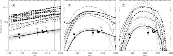
Figure 3. Dashed lines show predicted surface pressures for the (A) PNV (plus EPP1 and EPP2), (B) EPP (excepting EPP1 and EPP2), and (C) EEC runs; thick dashed lines show the 19 preferred runs. Solid lines show pressures scaled to pressures at 1275 km from stellar occultations; the thick, black solid lines show the example runs from Figure 1. Symbols show pressures at 1275 km derived from stellar occultations, from physical models (squares), simple parameterized atmospheres (following Elliot and Young 1992; filled circles), or the less accurate estimates from changes in half-light radius or scaling the pressures in a template atmosphere (open circles).
Download figure:
Standard image High-resolution image
After aphelion in the EPP and EEC runs, the summer (southern) hemisphere gets denuded near southern summer solstice, giving a period of cooling winter (northern) volatiles. This is followed by a period of rising pressures before perihelion equinox as the northern hemisphere gets more direct illumination. A southern volatile cap forms near the perihelion equinox. A period of exchange between the northern summer cap and the new southern winter cap ensues, with relatively stable surface pressures. The post-perihelion volatile migration mirrors the post-aphelion migration: the summer (northern) hemisphere disappears, the winter (southern) cap cools, the southern cap becomes more directly illuminated (transitioning from winter to summer), followed finally near aphelion by the exchange to a new winter (northern) hemisphere. All EEC runs have small N2 inventories (Figure 2(C)), allowing the post-perihelion northern summer cap to recede shortly after it begins transferring mass to the new southern winter cap.
4. COMPARISONS WITH OBSERVATIONS
Modeled pressures are compared against the occultation record in Figure 3, where the modeled surface pressures are plotted as dashed lines. Pressures derived from occultations since 1988 (Table 2) are reported at a reference radius of 1275 km from Pluto's center, since stellar occultations do not probe to Pluto's surface. The symbol types represent the analysis used to derive the pressures. For each run, I multiply the surface pressures by a single scale factor to compare with observations (solid lines). This assumes a constant ratio between the pressures at the surface and those measured at 1275 km, although this assumption is challenged by the simulated occultation light curves of Zalucha et al. (2011). Future atmospheric modeling will guide more accurate scaling from surface pressures at occultation levels aided by measurements of Pluto's radius and near-surface atmospheric structure by New Horizons (Young et al. 2008b). This will also be aided by measurements of Pluto's radius and near-surface atmospheric structure by New Horizons (Young et al. 2008b). The PNV pressures are in general agreement with the occultation record. The pressures from the EPP category are also consistent with the occultation record, within the measurement and modeling uncertainties of the occultations. The runs in the EEC category cannot be ruled out from occultation record at the 3σ level. An occultation in hand from 2011 June 23 had chords all one side of the occultation midline, making geometric reconstruction too inaccurate for use here. Another occultation from 2012 September 9 is currently being analyzed. The ECC solution predicts pressures in 2013 a factor of two lower than the 1988 occultation, and therefore analysis from 2013 onward should unambiguously test the EEC case. Reanalysis of the Pluto occultation of 1985 (Brosch 1995), while only a single chord taken under difficult conditions, might also be illuminating, as the EEC runs predict a factor-of-seven change in the pressure between 1985 and 1988.
Table 2. Pressures at Reference Altitude 1275 km from Pluto's Center, Measured by Stellar Occultation
| Date | Pressure at 1275 km | Analysis Type | Reference |
|---|---|---|---|
| (μbar) | |||
| 1988 Jun 9 | 0.83 ± 0.11 | EY92 model | Elliot & Young 1992 |
 |
Physical model | Zalucha et al. 2011 | |
| 2002 Aug 21 | 1.76 ± 0.51 | EY92 model | Elliot et al. 2003a |
 |
Physical model | Zalucha et al. 2011 | |
| 2006 Jun 12 | 1.86 ± 0.10 | EY92 model | Young et al. 2008a |
 |
Physical model | Zalucha et al. 2011 | |
| 2007 Mar 18 | 2.03 ± 0.2 | EY92 model | Person et al. 2008 |
| 2007 Jul 31 | 2.09 ± 0.09 | EY92 model | Olkin et al. 2013 |
| 2008 Aug 25 | 4.11 ± 0.54 | From half-light radius | Buie et al. 2009 |
| 2009 Apr 21 | 2.59 ± 0.09 | EY92 model | Young et al. 2009 |
| 2010 Feb 14 | 1.787 ± 0.076 | Temperature template | Young et al. 2010 |
Download table as: ASCIITypeset image
Pluto's surface has N2-rich, CH4-rich, and volatile-free terrains, with large longitudinal variation (Grundy et al. 2013; L11; Buie et al. 2010b). Quantitative comparisons between model and data for Pluto's albedo, color, thermal emission, and spectra will require models that include longitudinal variation and multiple volatile species. Still, broad constraints are provided by the current visible, thermal, and spectroscopic record, winnowing the parameter search to 19 preferred runs (Table 1).
The 80 year photometric record (Buratti et al. 2003; Schaefer et al. 2008; Buie et al. 2010a) and resolved maps from 1988, 1994, and 2002/2003 (Buie et al. 2010b) suggest that the low-contrast runs (EEC5) and very bright runs (PNV16, 17, 19, 21, 22, 23; EPP5, 8, 9, 10) are probably inconsistent with observed albedos. The maps and the secular changes in albedo suggest, in general, brighter poles and darker equatorial regions. All runs in Table 1 have bright northern volatile poles at the times of the maps, 1988–2002, except the dark-volatile EEC5 run. Runs that predict volatiles on the equator during 1998 and 2002/2003 (PNV4, 13, 16, 17, 19, 21, 23) are probably inconsistent with observations. A puzzle is that the southernmost latitudes are seen to be bright in the 1988 equinox maps, contrary to the predictions of this model. This may be an indication of bright substrate, as suspected near Triton's pole (Grundy & Young 2004). The EEC and some EPP runs predict diagnostic drops in albedo between 2000 and 2020; nearly all EPP and some PNV runs predict albedo drops before 2045.
Turning to Pluto's thermal emission, L11 find Γ ∼ 18 J m−2 s−1/2 K−1 from Spitzer observations, a value relevant to the diurnal skin depth (<90 cm; HP96). The values of Γ for PNV runs are high (nearly all in the range 316–3162 J m−2 s−1/2 K−1), but not implausible. The seasonal skin depth for these larger thermal inertia values is ∼100 m (HP96), so a PNV solution would require an increase of Γ with depth. In contrast, with the exception of the PNV-like EPP1 and EPP2, the EPP and EEC runs all have thermal inertia less than or equal to 100 J m−2 s−1/2 K−1. As it is unlikely that Γ decreases with depth, it is likely that only EPP1, 2, 3, 7, and 13 are plausible EPP solutions, and that EEC3, 4, 6, and 8 can also be eliminated. L11 find that Pluto's brightness temperature at 24 and 70 μm decreased between 2004 and 2007. Fourteen runs predict an increase in brightness temperature and may be less likely (PNV3, 18; EPP2, 10, 14, 16; EEC2, 3, 4, 5, 9, 10, 11, 12). Disk-integrated thermal emission is diagnostic on timescales of only three years. ALMA will be able to resolve Pluto's thermal emission, which will be even more constraining.
Near-infrared spectra of Pluto from 2001 to 2012 probe the CH4, CO, and N2 ices on Pluto (Grundy et al. 2013). The depth of the N2 ice absorption at 2.15 μm depends on the projected area of volatiles, and also their temperatures, grain sizes, and compositions. These competing factors make it more difficult to interpret the observed 25% decrease in the N2 absorption from ∼2004 to ∼2010 (Grundy et al. 2013). Detailed spectral modeling will yield more constraints. For now, I only suggest that runs that predict no northern cap in 2012 (EEC 5, 9, 10, and 11) are inconsistent with the presence of an N2 feature in the 2012 infrared spectrum.
5. PREDICTIONS FOR NEW HORIZONS
All PNV runs, the PNV-like EPP1 and EPP2, and the remaining higher-Γ EPP runs (EPP3, 7, 13) predict surface pressures greater than 10 μbar in 2015, well above the design specifications for the Alice and REX instruments on New Horizons (Young et al. 2008b). The runs in the EEC category all predict surface pressures less than 1 μbar in 2015. Despite the low pressures, only one run, EEC12, has a surface pressure too small to support a global atmosphere. For the others, volatiles only migrate from the edge of the winter cap toward the winter pole. The masses and the distances are small, so winds are subsonic. The Alice measurement of N2 opacity is effective even at these lower pressures, but, if the EEC models are correct, the REX instrument will measure near-surface pressures and temperatures with degraded sensitivity.
Most of the PNV runs have no volatiles on the southern hemisphere until several decades after the perihelion equinox. The implication is that much of the volatile migration at encounter will be from the directly illuminated high northern latitudes to the less directly illuminated edges of the northern volatile cap. The result may well be similar to that which Voyager saw at Triton, showing an old cap with a collar of new frost. For example, the run plotted in Figure 1 (PNV9) has subliming volatiles northward of 45° and condensing volatiles 21°–45°.
For the EPP runs (excluding the PNV-like EPP1 and EPP2), New Horizons might see an old, subliming, summer, northern pole, with just a sliver of the new, southern, winter pole visible. For the run plotted in Figure 1 (EPP7), the subliming pole extends northward from 20°, and the new, condensing pole extends southward from −15°.
For all the EEC runs, essentially by definition, the northern, summer volatile cap is completely or nearly completely sublimated in 2015. The EEC7 run plotted in Figure 1 has only one volatile pole, southward of −27°. There will be few N2-rich volatiles to be observed by the LEISA instrument on New Horizons. Note, however, that this version of the model does not track the CH4-rich volatiles, and these may remain on the visible hemisphere.
6. FUTURE WORK
New constraints from atmospheric pressures can come from new stellar occultations; new analysis of data from 1985 and 2012; application of atmospheric models to relate pressures at occultation altitudes to pressures at the surface; and New Horizons measurements of the near-surface atmosphere.
The inclusion of multiple species and longitudinal variation in volatile transport models will allow quantitative comparison to visible, thermal, and near-IR observations of Pluto's surface, including data from New Horizons.
Continuing ground-based observations of Pluto's surface and atmosphere will provide a temporal context in which to place the New Horizons flyby data. Conversely, New Horizons will provide a rich data set with which to understand Pluto's seasonal evolution.
This work was supported in part by NASA's New Horizons mission to the Pluto system and NASA Planetary Astronomy grant NNX12AG25G. The structure of the Letter was much improved by the suggestions of the anonymous referee.