SEASONAL CHANGES IN TITAN'S SURFACE TEMPERATURES

The primary goal of the Cassini mission is to study changes on Titan as it progresses from northern winter to summer. Major variations in Titan's weather can be expected during the extended mission, driven by seasonal shifts in surface heating. The small amount of sunlight that makes it through the atmospheric haze warms the surface, which in turn heats the lower troposphere and gives rise to atmospheric convection and circulation. Surface warmth lifts volatile materials, which condense to produce clouds and rain (Griffith et al. 2000; Brown et al. 2002). Meridional distributions of precipitation evolve globally as the insolation cycles through the Saturnian year. Modified appearances of surface features observed by Cassini have been associated with seasonal storms (Turtle et al. 2009, 2011), and the appearance of southern clouds has diminished in both Cassini and ground observations as Titan has progressed into southern autumn (Schaller et al. 2006; Rodriguez et al. 2009). In addition, warming of the surface governs wind patterns including dune-forming wind reversals and a seasonal shift of the intertropical convergence zone (ITCZ) that occur at the equinoxes (Mitchell et al. 2006, 2009; Tokano 2010). Seasonal changes in the atmosphere and on the surface are likely to accelerate as Titan moves toward northern summer.

Voyager 1 first measured the temperature of the surface of Titan through a spectral window of low atmospheric opacity at 19 μm (Samuelson et al. 1981; Flasar et al. 1981). From the single Voyager 1 encounter it was not possible to derive information about seasonal change, but the measurements showed a symmetric distribution around the equator as would be expected for the time of the flyby just after NSE. The Composite Infrared Spectrometer (CIRS; Flasar et al. 2004) aboard Cassini covers the 19 μm spectral window and has been recording spectra of Titan since 2004. We previously reported CIRS results from the 2004–2008 portion of the mission (Jennings et al. 2009) that gave a temperature of 93.7 K at the equator, in agreement with Huygens (Fulchignoni et al. 2005). The temperatures were 2 K cooler at the south pole and 3 K cooler at the north pole, appropriate to late northern winter. Titan has since advanced through NSE and into early northern spring, and the meridional distribution of surface temperatures is expected to have shifted northward significantly during that time. We present here evidence that the surface temperature is responding to the seasonal insolation shift and that the changes follow predictions from general circulation models (GCMs; Tokano 2005). Recently, Cottini et al. (2011) have reported spatial and temporal variations of surface temperature from CIRS measurements, including evidence of diurnal variations and seasonal shifts. Here, we extend their investigation of seasonal changes.

Surface brightness temperatures were derived from far-infrared observations by CIRS following the method described by Jennings et al. (2009). Spacecraft distances were constrained to be within 140,000 km of Titan to keep the 3.5 mrad field of view smaller than about 10% of the disk. The average emission angle viewed was restricted to <70° to limit the effect of the atmosphere. The surface radiances were measured in a channel centered on 530 cm^-1 with a bandwidth set by the 15 cm^-1 apodized resolution of the instrument. This spectral position is well within the 19 μm atmospheric window between the CH₄–N₂ and H₂–N₂ collisionally induced opacities (Courtin et al. 1995; Samuelson et al. 1997) and separated from HC₃N and C₂HD molecular emission below 520 cm⁻¹ (Kunde et al. 1981; Coustenis et al. 2008). The choice of 530 cm⁻¹ also permits direct comparison with previous work (Flasar et al. 1981; Jennings et al. 2009). On each Titan flyby only a limited latitude interval is observed and more than a year is typically required to cover the full pole-to-pole range. We have identified two distinct periods that each contain sufficient data to sample all latitudes and that are separated sufficiently in time to show a seasonal shift. These two periods are 2006 September through 2008 May, hereafter referred to as LNW, and 2008 November through 2010 May, hereafter called NSE. The periods are centered at solar longitudes L_s = 335° (0.8 Saturn month before NSE) and L_s = 0° (at NSE).

Radiance spectra in each time period were averaged zonally in 10° latitude bins before being converted to brightness temperature. We used larger latitude bins than the 5° bins in our previous study (Jennings et al. 2009) to improve the sensitivity of the results to seasonal change. Spectra in each latitude bin were averaged in two ranges of emission angle, 0°–50° and 50°–70°, and these were corrected separately for the effects of the atmosphere. To correct for the atmosphere we calculated the opacity and emission from the surface to space using the method described by Jennings et al. (2009), with several modifications to update our model atmosphere. As in the earlier work, we adopted the Huygens Atmospheric Structure Instrument (HASI) temperature profile for the equatorial region (Fulchignoni et al. 2005). This profile covers 0–147 km altitude. We then modified the temperature profile for higher latitudes to match the altitude behavior reported from Cassini Radio Science Subsystem (RSS) occultations (Flasar & Schinder 2010) and from CIRS molecular line retrievals (Achterberg et al. 2008, 2011; Anderson et al. 2010; Coustenis et al. 2010). We now include in our temperature model: (1) a large stratospheric variation in the north with a local maximum near 90 km and a local minimum near 120 km, (2) a middle troposphere (10–30 km) independent of latitude, and (3) a layer below 10 km where the lower atmospheric temperature transitions to the surface temperature. We adopted a haze opacity that increases downward with a scale height of 65 km above 80 km and remains constant from 80 km to the surface (Cottini et al. 2011; de Kok et al. 2007; Tomasko et al. 2005). In addition, we applied a latitude-dependent haze factor increasing by 50% from the south to the north, with a maximum at 40 N (Cottini et al. 2011; Rannou et al. 2010; Samuelson et al. 1997). The haze opacity was adjusted by an overall factor to produce the dependence of radiance on emission angle that we measure at the equator and at 73° N (Jennings et al. 2009). In our calculation of CH₄–N₂ opacity the methane mole fraction was updated to the dependence reported by Niemann et al. (2010): 1.48% above about 40 km rising to 5.65% below 7 km. The temperature dependent absorption coefficients for CH₄–N₂ from Borysow & Tang (1993) were increased by 50% as recommended by de Kok et al. (2010). For the H₂–N₂ opacity we used a mole fraction for molecular hydrogen (H₂) of 0.001 (Courtin et al. 1995; Jennings et al. 2009; Niemann et al. 2010) and assumed that it was constant over altitude and latitude. Temperature-dependent absorption coefficients for H₂–N₂ were taken from Courtin (1988) and Dore et al. (1986). We assumed the emissivity of the surface at 19 μm to be unity, which is justified because (1) our measured surface brightness temperature near the equator is the same as that measured at the surface by Huygens (93.7 K) and (2) our results are in agreement with near-surface radio occultation measurements (Flasar & Schinder 2010).

Figure 1 shows our derived surface brightness temperatures for the two periods. The temperatures for LNW are similar to those we previously reported for the first portion of the Cassini mission (Jennings et al. 2009). At the equator the temperature was ∼93.6 K, while at the south and north poles it was ∼91.5 and ∼90.5 K, respectively. However, between LNW and NSE it is evident that the temperatures increased in the north by roughly 0.5 K and decreased in the south by about the same amount. Equatorial temperatures may have decreased slightly, by about 0.2 K, possibly because Titan moved away from perihelion during this period. Although the maximum surface temperatures for both periods were near the equator, both profiles had generally higher temperatures in the south. The centroid of the temperature distribution, determined from cosine fits (as in Jennings et al. 2009), was located at 15° S latitude for LNW and 4° S for NSE. This gives a seasonal lag behind insolation of ΔL_S ∼ 9°. Our surface brightness temperatures are similar, in both seasonal lag and magnitude, to those of Voyager 1 Infrared Interferometer Spectrometer (IRIS; Flasar et al. 1981; Courtin & Kim 2002). Voyager 1 observed a roughly symmetric distribution about the equator at L_S = 10° with temperatures ranging from about 91–93 K for ±60° latitude. We conclude that the surface temperatures are repeating after one Saturn year, both in amplitude and seasonal lag.

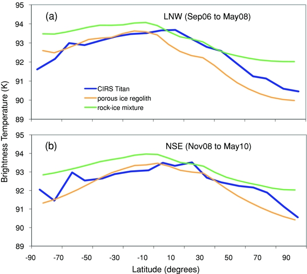
Zoom In Zoom Out Reset image size

Figure 2 shows our surface brightness temperatures compared with two surface composition scenarios of Tokano (2005): porous ice regolith and rock–ice mixture. Both LNW and NSE are compared with the GCM predictions for the same solar longitude. We find that the distribution of the observed surface temperatures has tracked the predictions quite closely. The distinction between the two scenarios lies in the thermal inertia, which is eight times higher for rock–ice mixture than for porous ice regolith (with an assumed thermal inertia of ∼330 J m⁻² s^−0.5 K⁻¹) due to the high heat conductivity of ice and higher compaction. In both time periods the measured equator-to-pole variations match the porous ice regolith scenario more closely than the rock–ice mixture. However, while the observations are closer to porous ice regolith in the south, in the north they tend to lie between the two scenarios. Although this might imply a difference in composition between the north and south, we are not sure that the accuracies of the data or the model warrant such a conclusion. In terms of seasonal lag, a cosine fit to the GCM predictions for a porous ice regolith shows a north–south symmetry at L_S ∼ 13°, in agreement with our derived ΔL_S ∼ 9° within uncertainties. In contrast, the predictions for a rock–ice mixture are symmetric at L_S ∼ 30°, inconsistent with both our results and those of Voyager 1 IRIS.

Zoom In Zoom Out Reset image size

The temperatures at the poles in both the LNW and NSE measurements are near the triple points for methane (90.6 K) and ethane (89.9 K), suggesting that gaseous and condensed phases might exist together on the surface at high latitudes. A ∼0.5 K change (our observed increase in the north and decrease in the south) corresponds to a 7% change in saturation vapor pressure for methane and 14% change for ethane. Evaporation and condensation rates are therefore likely to have already been affected by the seasonal advancement. By the end of the Cassini mission, at summer solstice, the poles may have changed by as much as 3 K from the LNW values (Tokano 2005). This represents a 50% change in vapor pressure for methane and a factor of two for ethane. Thus, we can expect major changes in condensed phases at high latitudes during the remainder of the mission.

Some features in our observed surface temperatures may be related to cloud distribution. In the south the latitude bin at 60°–70° S is elevated in temperature relative to its neighbors during both LNW and NSE, by about 0.5 and 0.7 K, respectively. We note that this latitude coincides with a relatively cloud-free gap between two zones where clouds commonly appear, one zone centered at ∼40° S and another region extending poleward from ∼70° S (Rodriguez et al. 2009; Griffith et al. 2005; Roe et al. 2005). An elevated surface temperature at 65° S might be the result of higher insolation in the cloud-free zone. As northern summer approaches the atmospheric circulation patterns are expected to change and the temperature peak at 65° S may migrate in latitude or disappear.

In the north the largest temperature changes are at higher latitudes, >40° N. In fact, we see no changes greater than the errors in the two bins centered at 25° and 35° N, possibly because the increase in solar declination is compensated by the increasing solar distance. The temperature variation is greatest at 50°–70° N, but is small again at 70°–90° N. At these highest latitudes the changes are less than predicted for land composed only of porous ice regolith. This may result in part from the large fraction of lake surface at the northernmost latitudes. During the winter the polar lakes are expected to have a temperature similar to that of the land. However, in the spring the warming of the lakes is slower than the land due to their larger thermal inertia (Tokano 2009). The predicted lake temperature is 90–91 K throughout winter and early spring, and begins to increase only in late spring. Our results so far are consistent with this prediction, implying that the large lake coverage effectively increases the thermal inertia near the pole. By the end of the Cassini mission we may begin to see evidence of rising temperatures in the polar lakes.

We acknowledge support from NASA's Cassini mission and Cassini Data Analysis Program. T.T. was supported by DFG.