

Abstract
Development of the measurement-based carbon accounting means is of great importance to supplement the traditional inventory compilation. Mobile CO2/CH4 measurement provides a flexible way to inspect plant-scale CO2/CH4 emissions without the need to notify factories. In 2021, our team used a vehicle-based monitor system to conduct field campaigns in two cities and one industrial park in China, totaling 1143 km. Furthermore, we designed a model based on sample concentrations to evaluate CO2/CH4 emissions, EMISSION-PARTITION, which can be used to determine global optimal emission intensity and related dispersion parameters via intelligent algorithm (particle swarm optimization) and interior point penalty function. We evaluated the performance of EMISSION-PARTITION in chemical, coal washing, and waste incineration plants. The correlations between measured samples and rebuilt simulated ones were larger than 0.76, and RMSE was less than 11.7 mg m−3, even with much fewer samples (25). This study demonstrated the wide applications of a vehicle-based monitoring system in detecting greenhouse gas emission sources.
Export citation and abstract BibTeX RIS

Original content from this work may be used under the terms of the Creative Commons Attribution 4.0 license. Any further distribution of this work must maintain attribution to the author(s) and the title of the work, journal citation and DOI.
1. Introduction
The IPCC 5th assessment report states that greenhouse gases (GHGs) from anthropogenic production activities have a significant impact on global climate change (IPCC 2014), continuously increasing GHGs would enforce the greenhouse warming effect that leads to sea-level rise and extreme weather (Kemper 2015, Nerem et al 2018). Efficient assessment of the emission intensity of the most important GHGs, CO2 and CH4, will be important for the formulation of policies to protect the environment (Le Quéré et al 2009, Gorchov Negron et al 2020, Liu et al 2020). Strong point source emission types account for the majority of total anthropogenic emissions, such as fossil combustion emissions from industrial production and methane leakage from human mine extraction (Schwandner et al 2017, Delgado et al 2018, Cheng et al 2021). The current methods for quantifying such emission intensities rely on emission inventories methods, such as the Open-source Data Inventory for Anthropogenic CO2 (ODIAC), Emissions Database for Global Atmospheric Research (EDGAR), and Multi-resolution Emission Inventory for Chin (MEIC) (Oda et al 2018, Zheng et al 2020). Inventories are critical in analyzing the annual or monthly emission intensity of the concerned sources, which could represent the general emission characteristic. However, high timeliness emission reports would be benefited for energy evaluating and environment protect sectors (Goldberg et al 2019).
The 'top–down' assessment of emission sources through concentration data has evolved into a reliable methodology with real-time results and high accuracy. Satellite remote sensing allows for quantifying point sources based on the measured GHG concentrations under specific detection orbits and meteorological conditions (Nassar et al 2017, Zheng et al 2020). However, current GHG satellites (Wunch et al 2017), like Orbiting Carbon Observatory-2 (OCO-2), the Greenhouse Gases Observing Satellite (GOSAT), and Tropospheric Monitoring Instrument (TROPOMI), are susceptible to environmental factors such as clouds, aerosols, and solar radiation intensity, which can limit targeted monitoring of concerning areas (Crisp et al 2017). Airborne remote sensing methods can be used to record large-scale GHG fluxes, such as the German Methane Airborne MAPper passive observation approach to obtain methane fluxes in the Upper Silesian Coal Basin (Krautwurst et al 2021). CO2 and CH4 Atmospheric Remote Monitoring Flugzeug (CHARM-F), an integrated path differential absorption LiDAR, retrieves carbon emissions from power plants in Germany (Wolff et al 2021). However, the airborne remote sensing methods have high technical requirements, high cutting costs, and cannot monitor emission sources long-term. Unmanned aerial vehicle (UAV) gas sampling systems have high flexibility to capture different spatial gas concentration distributions (Andersen et al 2021). In combination with diffusion models or flux calculation methods, emissions from strong methane sources, such as mines and dairy farms (Vinkovic et al 2022), could be evaluated using an UAV-based Aircore system, but UAV devices can only monitor emission sources on a small-scale.
Ground-based monitoring systems act like a network of in situ sensors allowing for regional carbon flux assessment in cities (Turner et al 2016), but establishing sensor networks for strong point source emissions is less cost-effective. Brantleyt et al presented a vehicle-based sampling system with an in situ sensor and 3D meteorological instruments to measure methane emission leakage due to oil and gas production (Brantley et al 2014a). This system could sample GHGs with high accuracy, and the detected track could be freely planned to ensure that the number of samples in the quantification models is sufficient (Albertson et al 2016). However, the emission quantification model used in this system, named other test method 33 A model (OTM33A), requires a large amount of samples and prior information in the vicinity of specific emission sources. Our team developed a vehicle-based gas sampling system that can measure CO2 and CH4 concentrations simultaneously. Based on the Gaussian diffusion model and few samples, we designed a fast and highly accurate evaluation model for GHG emissions.
Gaussian diffusion models are currently the dominant point source diffusion models, but their core diffusion parameters are often calculated based on empirical formulas (Magazine 1961, Bovensmann et al 2010, Nassar et al 2021). This is not reasonable regardless of the actual measured scenario about the emission source, which will cause additional errors in gas emission quantification (Pei et al 2022). In addition, the accuracy of wind speed and direction also has a large impact on the retrieved emission value (Varon et al 2018, Wang et al 2018, Wu et al 2022). Tackling with the above shortcomings, we developed an adaptive multi-source Gaussian diffusion model based on the PARticle swarm opTimization and interior poInt penalTy functION, named EMISSION-PARTITION, which can obtain robust emission rates with hardly prior information. Such features provide us a novel and independent identification/verification means for anthropogenic GHG emissions.
2. Method
2.1. Vehicle-based monitoring system
The vehicle-based GHG emission monitoring system (VGMS) contains four parts: an electric bus, in situ sensor (PICARRO G2201-i), meteorological instrument, and global positioning system (GPS) (see figure 1(a)). PICARRO G2201-i could sample CO2 and CH4 simultaneously. For CO2, the accuracy of samples is ±0.2 parts per million (ppm). For CH4, the accuracy of samples is ±5.0 parts per billion. The meteorological instrument collects ambient temperature, ambient pressure, ambient relative humidity, wind speed, and wind direction. A GPS records the location of sample points during the measured track.
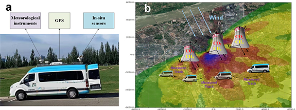
Figure 1. Vehicle-based monitoring system and measured circumstances.
Download figure:
Standard image High-resolution image2.2. Description of field studies
VGMS has collected the GHG distribution in three field campaigns, including the cities in Inner Mongolia (A), Hebei (B), and Liaoning (C) in China, see figure 2. These three cities have different industries and factories. The amount of coal mined in A could reach 6.5 billion tons per year, and crude steel production in B was more than 1.30 billion tons in 2021. The main purpose of the field experiments is quantifying CO2 emissions from industrial parks and methane leakage from some energy conversion units. Therefore, sample tracks of VGMS contain the GCD industry peak and LG factories, ZN steel factory, ZN Chemical Plant, and XC waste incineration plant.
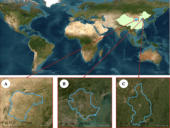
Figure 2. Measured sites of VGMS, including cites of A,B and C.
Download figure:
Standard image High-resolution imageFrom August 2021 to December 2021, four monitoring experiments were conducted by our group, as shown in table 2. It worth noting that the Picarro analyzer was calibrated by the standard concentration of GHGs in each track, see S3. In addition, the anomalous values caused by vehicle emissions around the sampling vehicle were removed during the measurements.
2.3. Emission quantification model
The diffusion of gases emitted from strong emission sources could be modeled by a multi-sources Gaussian dispersion model (formula (1)):


The coordinate system of the field campaign is set according to the location of emission source and wind direction (figure 1(b)). The location of each emission source is set as the coordinate origin (O) in its corresponding coordinate system, wind direction is set as the X axis, Y is perpendicular to the X axis, and Z is perpendicular to XOY. C(m) is GHG concentration of the mth samples, Qi
is GHG emission intensity of the ith point source, for i = 1,2,3 ...n, n is total number of strong point sources; u is the wind speed, Hi
is the effective GHG emission height of the ith point source,  and
and  are the horizontal and vertical diffusion parameters that refer to the ith point source, respectively, B is the background concentration of GHG in the measured area, a, b is the horizontal diffusion coefficient, and c, d is the vertical diffusion coefficient.
To solve for the unknown parameters in formulas (1)–(3), including Qi, Hi, a, b, c, d, and B, EMISSION-PARTITION, see figure 3, whose kernel is particle swarm optimization (PSO) coupled with interior point penalty function (IPPF). First, the potential range of unknown parameters are defined according to PSO model, and the fitness value of PSO was set as formula (4), see S1 in supplementary:
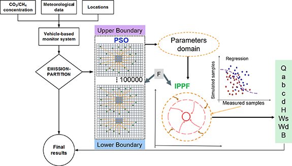
Figure 3. Framework of the EMISSION-PARTITION.
Download figure:
Standard image High-resolution imageC(k) is the actual measured samples, C'(k) is the simulated concentration, m is the total number of the selected concentration samples used to retrieve emission rate. This step is repeated 100 000 times to acquire the Parameters domain of each unknown parameter. Then, the solution of unknown parameters is further determined by IPPF function, and the penalty function of IPPF in this step also refers to formula (4). Results of unknown parameters could be retrieved when F achieved the minimum value.
2.3.1. Uncertainty analysis
Formula (5) was used to determine the uncertainty of quantified emission rate through relevant variables in actual experiments:
 t
is defined uncertainty of retrieved emission rate, and n, m, w
, and d
represent the uncertainty caused by number of samples, accuracy of samples, wind speed, and wind direction, respectively. It is noted that the uncertainty of each item was referring to the corresponding value in sensitivity analysis, see section 3.2. Uncertainties of wind speed and direction are defined by standard deviation of 2 min collections of wind speed and direction around the emission source. Uncertainty of sample accuracy is referenced by the calibrated experiment of PICARRO by standard gases, which is about 0.1%. We presented the detailed processes in calculating t
in S2.
t
is defined uncertainty of retrieved emission rate, and n, m, w
, and d
represent the uncertainty caused by number of samples, accuracy of samples, wind speed, and wind direction, respectively. It is noted that the uncertainty of each item was referring to the corresponding value in sensitivity analysis, see section 3.2. Uncertainties of wind speed and direction are defined by standard deviation of 2 min collections of wind speed and direction around the emission source. Uncertainty of sample accuracy is referenced by the calibrated experiment of PICARRO by standard gases, which is about 0.1%. We presented the detailed processes in calculating t
in S2.
3. Results
3.1. Observing system simulation experiments (OSSE) to test EMISSION-PARTITION
In this section, we take CO2 emission source quantification as an example. First, we set up different numbers of emission sources, including 1, 2, and 3. Then, we generated simulated values of CO2 concentration downwind according to formula (1) based on the parameters (true values) shown in table 1; the spatial resolution was 2 m. Then, 150 simulated points were randomly selected, and a relative error of 1.5% was added for the hypothetical measurement points. In order to make OSSE close to the real measurement scene, we set the uncertainty of wind speed as ±0.5 m s−1 and the uncertainty of wind direction as ±50°. It is worth noting that the uncertainty was far larger than that of actual meteorological instruments. The lower and upper boundary of each parameter was set as shown in table 1. Then, the unknown parameters were calculated by EMISSION-PARTITION and repeated 10 000 times. Finally, the mean value of the retrieved Q was treated as the final retrieved value (see table 2).
Table 1. Detailed information in actual field campaign.
| Date | Measured sites | Sample period | Gases |
|---|---|---|---|
| 22th August, 2021 | A | 278 min 59 s | CO2/CH4 |
| 8th December, 2021 | B | 497 min 21 s | CO2 |
| 16th December, 2021 | South C | 241 min 42 s | CO2/CH4 |
| 17th December, 2021 | West C | 483 min 02 s | CO2/CH4 |
Table 2. Parameters in OSSE and results calculated by EMISSION-PARTITION.
| Parameters | True value | Lower boundary | Upper boundary | Retrievals | Standard deviation | |
|---|---|---|---|---|---|---|
| Ws (m s−1) | 3.0 | 1.5 | 3.5 | 2.6 | 0.2 | |
| Wd (°) | 90 | 40 | 140 | 90 | 1.0 | |
| a | 0.2 | 0 | 100 | 0.21 | 0.02 | |
| b | 0.9 | 0 | 100 | 0.88 | 0.03 | |
| c | 0.1 | 0 | 100 | 0.1 | 0.01 | |
| d | 0.9 | 0 | 100 | 0.91 | 0.02 | |
| H (m) | 15 | 0 | 100 | 14.3 | 1.2 | |
| B (g m−3) | 813 | 785 | 845 | 815.2 | 2.4 | |
| 1 source | Q (kg s−1) | 60 | 0 | Inf | 60.4 | 1.3 |
| 2 sources | Q2_1 (kg s−1) | 100 | 0 | Inf | 98.2 | 1.8 |
| Q2_2 (kg s−1) | 50 | 0 | Inf | 51.4 | 1.5 | |
| 3 sources | Q3_1 (kg s−1) | 100 | 0 | Inf | 102.3 | 2.1 |
| Q3_2 (kg s−1) | 50 | 0 | Inf | 48.5 | 1.8 | |
| Q3_3 (kg s−1) | 30 | 0 | Inf | 29.2 | 1.1 | |
The conventional diffusion parameters (a, b, c, and d) are empirically determined based on atmospheric stability. There is a large uncertainty due to the topographic characteristics of the studied area, solar radiation energy, different types of emission sources, etc.
As shown in table 1, the values of a, b, c, and d are nearly the same as the settings, and the maximum of standard deviation is only 0.01, indicating that EMISSION-PARTITION can calculate diffusion parameters without prior information. In addition, the retrieved H was also accurate, with only a 0.7 m bias to 15.0 m, which helps to reconstruct CO2 diffusion from emission sources. It is worth noting that the accuracy of the solution of the emission sources will decrease with the increase in number of emission sources, because more emission sources will bring additional parameters in the solutions by EMISSION-PARTITION. As shown in table 1, even in the case of three emission sources, the accuracy of retrieved emission rates was still better than 2.7%, with a standard deviation of less than 4%. In summary, the EMISSION-PARTITION has a self-adjusting function to reach the optimal solutions in unknown parameters and reduce the uncertainties in final retrievals.
3.2. Sensitivity analysis
In the actual field campaign, the concentrations of samples of gases and meteorological factors would be influenced by the performance of the equipped instruments in the vehicle-based monitoring system. In this section, we evaluate the stability of the EMISSION-FUN model with different measured parameters, and we analyzed the uncertainties of different wind speeds, wind directions, and sampling accuracy, and the influence of different sampling quantities on the final emission assessment. Here, we take a single point source as an example and use the control variables method for sensitivity analysis of the analyzed parameters. The average of 10 000 repetitions was used as the inverse result, and the standard deviation was calculated based on the results of 10 000 repetitions.
As shown in figure 4(a), we analyzed the effect of different errors in wind speed on final retrieved emission rate, and the uncertainty of the retrieved Q increases with the wind speed error. However, it is worth noting that even when uncertainty in wind speed is 1.6 m s−1, with a 53% bias to 3.0 m s−1, the retrieved Q has 2.5 kg s−1 bias to the actual value, and the standard deviation is only 3.1 kg s−1. EMISSION-PARTITION is not sensitive to the additional errors in wind directions (figure 4(b)); the retrieved emission rates are in the range of 59.8–60.74 kg s−1, and the standard deviations of emission rates are less than 0.34 kg s−1. The number of samples and the sampling accuracy determine limiting equations and accuracy of the basis of judgment in the EMISSION-PARTITION solution process. As shown in figure 3(c), the standard deviation of Q increases with the additional errors in samples, but even with a sampling error of 6%, the standard deviation of Q is only 2.1 kg s−1. The number of samples has the largest impact on the final emission inversion (figure 4(d)). For example, the standard deviation can reach 15.2 kg s−1 when the number of samples is 20, but it would be less than 0.7 kg s−1 if the number of samples was more than 120. In general, EMISSION-PARTITION can improve the accuracy of the emission intensity by adjusting the input parameters dynamically according to the PSO algorithm and achieving the global optimal solution according to the IPPF.
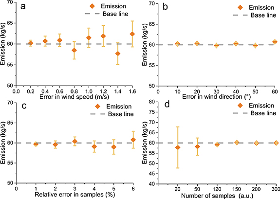
Figure 4. Influence of different parameters settings on retrieved emission rate. (a) Additional errors in wind speed; (b) additional errors in wind direction; (c) additional errors in samples; (d) amount of CO2 samples collected by vehicle-based monitoring system.
Download figure:
Standard image High-resolution image3.3. Actual cases
As shown in figure 5, the CO2 concentrations collected by our monitoring system have a large variation range in all field campaigns, for example, 425–520 ppm in B. CO2 concentration are higher in urban areas (figures 5(b)–(d)) because of multiple irregularities in urban emission sources in cities and sampling time is winter. Both B and C countries have large amounts of heating equipment, and the enhanced CO2 values from these emission sources have been acquired by the monitoring system. Samples on roads show the lowest values, which are smaller than those in the industrial park, due to strong emission sources in the industrial park. Overall, the vehicle-based monitor can obtain CO2 distribution characteristics under different land use types.
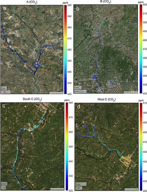
Figure 5. Samples of CO2 in different field campaigns; (a) A; (b) B; (c) South C; and (d) West C.
Download figure:
Standard image High-resolution image3.3.1. CH4 distribution
Because CH4 was not sampled in the B field campaign, only A and two tracks in C were analyzed in this section. In figure 6, similar to CO2, CH4 concentration is also higher in urban areas, for example, it could be up to 2.61 ppm in the main city of C. This is due to methane production from gas leaks or garbage fermentation in residential areas. It is noteworthy that samples around factories in C do not show strong CH4 enhancement values, which may be caused by their energy consumption; most factories use solid fossil fuels to serve as energy for production. The vehicle-based monitoring system only detected enhanced CH4 concentration in the industrial park of A, ZN Chemical Plan.
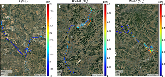
Figure 6. Samples of CH4 in different field campaigns; (a) A; (b) South C; and (c) West C.
Download figure:
Standard image High-resolution image3.4. Emission quantification
Based on the field campaign presented in figures 4 and 5, the quantitative assessment in different numbers of emission sources was performed based on EMISSION-PARTITION, which contains chemical plants, waste incineration plants, and coal washing plants.
3.4.1. Single CO2 emission source
In section 3.2 it is shown that more samples will lead to higher accuracy and stability in quantifying emission rate, and this has also been validated in actual cases. Two hundred and five samples were collected for the ZN Chemical Plant, while only 25 samples were measured around the XF waste incineration plant. In figures 7(c) and (f), we can also see that the CO2 point source diffusion reconstruction for the ZN Chemical Plant is much better than that for the XF Waste Incineration Plant. The R2 in figure 7(c) is higher than the R2 in figure 7(f), and the RMSE is only 0.03 mg m−3 in figure 7(c) and 11.7 mg m−3 in figure 7(f). This indicates that a high sampling rate will help to reduce the uncertainty of emission assessment.
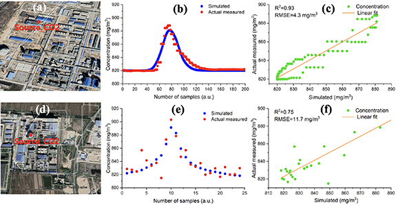
Figure 7. Single CO2 emission source. (a)–(c), ZN chemical plant, (a) location of CO2 source, (b) simulated CO2 concentration and actual CO2 samples (c). Correlation between simulated CO2 concentration and actual CO2 samples. (d)–(f), XF waste incineration plant, (d) location of CO2 source, (e) simulated CO2 concentration and actual CO2 samples (f). Correlation between simulated CO2 concentration and actual CO2 samples.
Download figure:
Standard image High-resolution image3.4.2. Multi-point CO2 emission sources
The two CO2 emission sources in the MX coal washing plant are mainly the two coal crusher machines. In this case, the amount of samples is 125 for quantifying CO2 emission rate. The R2 is 0.92 and RMSE is 10.4 mg m−3, which show less consistency than that shown in figure 7(c). The additional emission source and fewer samples would reduce useful residual observation restrictions.
Figure 8(d) represents triple CO2 emission sources in the ZN Chemical plant, and the number of selected samples for quantification is 300. As shown in figure 8(e), the values of samples are much larger than those in previous cases. The distance between the emission source and vehicle monitoring system is extremely small, and the minimum value is only 26 m. In figure 8(f), although R2 is 0.89, RMSE is 46.3 mg m−3. Firstly, the number of unknown parameters in this case is the greatest; a smaller distance between samples and emission sources would lead to unstable diffusion of CO2. This case indicates that a closer proximity of samples around the emission source is not always beneficial for emission quantification.
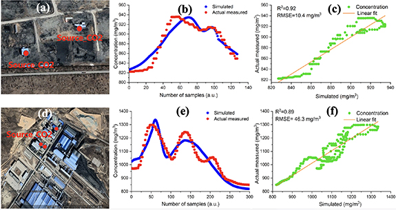
Figure 8. Multi-point CO2 emission sources. (a)–(c), MX coal washing plant, (a) locations of CO2 source, (b) simulated CO2 concentration and actual CO2 samples, (c) correlation between simulated CO2 concentration and actual CO2 samples. (d)–(f) ZN chemical plant, (d) location of CO2 source, (e) simulated CO2 concentration and actual CO2 samples, (f) correlation between simulated CO2 concentration and actual CO2 samples.
Download figure:
Standard image High-resolution image3.4.3. Single CH4 emission source
Two CH4 enhancements due to strong emission sources were observed during the A cruise, both of them in the ZN chemical plant. The main operation of this plant is gas coal liquefaction, which may cause leakage during the liquefying process. As is shown in figure 9, the vehicle-based monitoring system has the ability to capture the enhanced methane concentration adequately, with more than 200 samples of enhancement for each source. The R2 between results calculated by EMISSION-PARTITION and the actual samples is greater than 0.96, and RMSEs are not larger than 0.04 mg m−3. This demonstrates that for a single methane source, a good inverse response can be obtained with sufficient sampling. It is proven that for a single methane source, the EMISSION-PARTITION can rebuild the dispersion of methane with reliable performance.
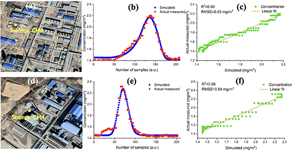
Figure 9. Single CH4 emission source. (a)–(c), ZN chemical plant, (a) location of CH4 source, (b) simulated CH4 concentration and actual CH4 samples, (c) correlation between simulated CH4 concentration and actual CH4 samples. (d)–(f), ZN chemical plant (d) location of CH4 source. (e) Simulated CH4 concentration and actual CH4 samples. (f) Correlation between simulated CH4 concentration and actual CH4 samples.
Download figure:
Standard image High-resolution image3.4.4. Summary of the emission rate
Table 3 shows the retrieved emission rate and dispersion coefficients in all cases. Among them, positions of case 1 and 5 are very close in A, and retrieved wind speed and wind direction in the two cases are almost the same. The background concentrations in the same area also show good agreement, such as in case 1 and 3, and in case 4, the ZN chemical plant, the maximum difference of B of CO2 in the three cases is only 2.9 mg m−3. The consistency of wind and B proved the rationality of EMISSION-PARTITION. Among all CO2 emission sources, the XF waste incineration plant has the highest emission intensity of 22.3 kg s−1. The emission rates of three emission sources (case 4) can still be quantified even though the values are low. The emission rates of CH4 at both ZN chemical plants were larger than 1 and less than 2 g s−1, which were similar to the reported results of oil and gases produced in the United States (Albertson et al 2016).
Table 3. Emission rate and diffusion parameters in 6 Cases.
| Gases | Cases | Q | Ws (m s−1) | Wd (°) | a | b | c | d | H (m) | B (mg m−3) |
|---|---|---|---|---|---|---|---|---|---|---|
| CO2 | 1 | 4.8 kg s−1 | 2.2 | 137.2 | 0.1 | 0.95 | 0.40 | 1.10 | 5.20 | 820.2 |
| 2 | 22.3 kg s−1 | 3.1 | 97.9 | 0.12 | 1.15 | 0.7 | 0.3 | 25.6 | 822.4 | |
| 3 | Q3_1:5.1 kg s−1 | 2.0 | 166.2 | 0.1 | 1.18 | 0.06 | 1.2 | 12.6 | 817.3 | |
| Q3_2: 5.6 kg s−1 | ||||||||||
| 4 | Q4_1:2.3 kg s−1 | 2.3 | 127.4 | 0.21 | 1.18 | 0.24 | 0.9 | 12.8 | 818.4 | |
| Q4_2: 1.8 kg s−1 | ||||||||||
| Q4_3: 0.9 kg s−1 | ||||||||||
| CH4 | 5 | 1.1 g s−1 | 2.2 | 136.8 | 0.12 | 1.35 | 0.06 | 0.75 | 3.1 | 1.45 |
| 6 | 1.4 g s−1 | 2.4 | 123.4 | 0.28 | 1.13 | 0.30 | 0.93 | 19.3 | 1.43 |
4. Discussion
We demonstrated the self-adjusted function of EMISSION-PARTITION model for input parameters in section 3, and verified the reconstruction capability of GHGs diffusion in real cases. To further evaluate the reliability as well as the advantage of the proposed model, we need to compare the retrieved results with other methods and present the potential applications in actual scenarios.
4.1. Comparison with other methods
We quantified the emission rate from single point sources with similar methods, including the other test method (OTM) 33 A model proposed by the US EPA and IPPF model developed by Shi et al 2022, Brantley et al 2014b, Shi et al 2021).
4.1.1. OTM33A
The main principle of OTM33A is getting the peak GHG concentration among the samples based on the Gaussian fitting, and then the emission rate is calculated by an integral with two dimensions (formula (6)). The diffusion parameters σy and σz are regarded as certain values by the distance from the source and different atmospheric stabilities, which are determined by CH4 control-release experiments by the EPA:
y is crosswind distance (m), z is vertical distance (m), a1 is peak average methane concentration (g m−3) as determined by Gaussian fit, σy is standard deviation of the crosswind plume concentration (m), and σz is standard deviation of the vertical plume concentration (m).
4.1.2. IPPF
Based on the network of gas sensors and Gaussian dispersion model, the IPPF model could also be used to obtain the emission rate and diffusion parameters using a single strong point source (see formula (5)). However, the values of a, b, c, and d are restricted according to the Pasquill method and GB3840-83 (China) (Hanna et al 1982, Shi et al 2020).
As is shown in figure 10(a), emission rates of ZN are 4.3 ± 0.4, 3.2 ± 1.2, and 7.1 ± 2.4 kg s−1 calculated by EMISSION-PARTITION, IPPF, and OTM33A, respectively. The emission rate of XC calculated by EMISSION-PARTITION, 22.3 ± 6.4 kg s−1, is lower than that calculated by the other two methods. It is worth nothing that OTM33A would always overestimate the emission rate in two cases, because the values of σy and σz in OTM33A are defined by EPA experiments of CH4 diffusion and are larger than those of CO2. Comparing the quantified emission rates of CH4, the mean difference of the two cases is about 0.5 g s−1. Notably, EMISSION-PARTITION has the significant benefit of the lowest uncertainty among the three methods.

Figure 10. Results of GHG emission based on different methods. (a) CO2; (b) CH4.
Download figure:
Standard image High-resolution image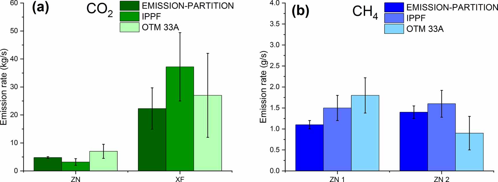
4.2. Application of proposed program
The increasing greenhouse effect will cause various ecological problems and threaten human environments (Liu et al 2022). Energy saving and emission reduction are important measures to mitigate this hazard. As a first step, we need to precisely assess current GHG emissions from different sectors, which are not reliable and quantifiable because of the imperfect construction of various GHG emission inventories in developing countries (Su et al 2017). This is detrimental to the formulation of environmental policies and improvement in global climate change (Luo et al 2022). This study presented a movable vehicle-based monitoring system and EMISSION-PARTITION model, which can quickly assess the emission intensity of strong sources based on the concentration data collected in real time. This program has high flexibility to realize the monitoring function, provide data support for governments, promote the improvement of timeliness and accuracy of self-announced emissions in developing and developed countries, establish penalty mechanisms, and finally, urge enterprises and factories to complete the conversion from reliance on oil and fossil fuels to clean energy (Xiao et al 2021). In the future, our developed vehicle-based monitoring system could include in situ sensors for pollutant gases, such as NO2, CO, and SO2, to simultaneously evaluate the emission rate of pollutant gas and GHG and assess energy use efficiency.
5. Conclusion
In this study, we presented multi-source GHGs emission quantification model, named EMISSION-PARTITION, which could retrieve emission intensity from strong sources through GHGs concentration samples. We concluded that amount of samples is an important factor that influence the accuracy of final retrieved emissions. Actual field campaigns validated the reliable performance of proposed model in retrieving CO2/CH4 source emissions through our developed vehicle monitoring system, which contains chemical plants, waste incineration plants, and coal washing plants. Uncertainty of retrieved emissions intensities would be less than 17.3%, we believe multi overpass of vehicle monitoring system around the emission source would be helpful in improving the accuracy of emission quantification in future. EMISSION-PARTITION could also quantify GHGs emission through other in-situ sampling systems, such as UAV-based Aircore or a network of in situ sensors. Consequently, similar programs are expected to enrich the categories of GHG inventory and evaluate energy loss in extraction, like calculating utilization efficiency of energy from industries and CH4 leakage from coal mining.
Data availability statement
The data cannot be made publicly available upon publication because they contain commercially sensitive information. The data that support the findings of this study are available upon reasonable request from the authors.
Acknowledgment
This study was funded by National key research and development program (Grant No. 2022YFB3904801), National Natural Science Foundation of China (Grant No. 41 971 283), the numerical calculations in this paper have been done on the supercomputing system in the Supercomputing Center of Wuhan University. Finally, we would also like to thank all reviewers for their constructive and valuable comments.
Supplementary data (0.1 MB PDF)