

Abstract
Global net-negative carbon emissions are prevalent in almost all emission pathways that meet the Paris temperature targets. In this paper, we generate and compare cost-effective emission pathways that satisfy two different types of climate targets. First, the common approach of a radiative forcing target that has to be met by the year 2100 (RF2100), and, second, a temperature ceiling target that has to be met over the entire period, avoiding any overshoot. Across two integrated assessment models (IAMs), we found that the amount of net-negative emissions—when global net emissions fall below zero—depends to a large extent on how the target is represented, i.e. implemented in the model. With a temperature ceiling (no temperature overshoot), net-negative emissions are limited and primarily a consequence of trade-offs with non-CO2 emissions, whereas net-negative emissions are significant for the RF2100 target (temperature overshoot). The difference becomes more pronounced with more stringent climate targets. This has important implications: more stringent near-term emission reductions are needed when a temperature ceiling is implemented compared to when an RF2100 target is implemented. Further, in one IAM, for our base case assumptions, the cost-effective negative carbon emissions (i.e. gross anthropogenic removals) do not depend to any significant extent on how the constraint is implemented, only, largely, on the ultimate stringency of the constraint. Hence, for a given climate target stringency in 2100, the RF2100 target and the temperature ceiling may result in essentially the same amount of negative carbon emissions. Finally, it is important that IAM demonstrate results for diverse ways of implementing a climate target, since the implementation has implications for the level of near-term emissions and the perceived need for net-negative emissions (beyond 2050).
Export citation and abstract BibTeX RIS

Original content from this work may be used under the terms of the Creative Commons Attribution 4.0 license. Any further distribution of this work must maintain attribution to the author(s) and the title of the work, journal citation and DOI.
1. Introduction
One objective of the Paris Agreement is to hold 'the increase in the global average temperature to well below 2 °C above pre-industrial levels and pursue efforts to limit the temperature increase to 1.5 °C above pre-industrial levels'. Many studies have identified technically feasible pathways to meet this Paris objective using integrated assessment models (IAMs) that combine economic, energy, climate and sometimes also land-use models. To represent the temperature goals, IAMs are often designed to meet a given radiative forcing (RF) level in the year 2100 (e.g. Riahi et al 2017), a concentration level (e.g. 450 ppm CO2-eq) in 2100 (e.g. Kriegler et al 2013), or stay within a given amount of cumulative emissions by 2100 (e.g. Bauer et al 2018, Luderer et al 2018). These targets are often implemented as physical constraints in an optimization model, or as carbon price pathways selected to meet the constraint. Generally, the temperature outcomes of the emission pathways generated by the IAMs are further evaluated ex-post using simple climate models (Rogelj et al 2018a). Some models have the ability to optimise towards a temperature target directly (Manne and Richels 2001, Azar et al 2013, Strefler et al 2014, Nordhaus 2018a), but this approach is less common in the recent literature. One plausible explanation for the focus on RF levels in 2100 is that this approach has played a dominant role in the scenario framework based on the Representative Concentration Pathways (RCPs), the Shared Socioeconomic Pathways (SSPs), and the Shared Policy Assumptions (SPAs) (Moss et al 2010, van Vuuren, 2014, Kriegler et al 2014).
Most emission pathways assessed in the IPCC Special Report on Global Warming of 1.5 °C (IPCC SR 1.5 °C) that keep the temperature increase below 1.5 °C of global warming in 2100 involve significant amounts of net-negative emissions. Note that there are two common uses of the term 'negative emissions'. One focuses on the overall anthropogenic removal of carbon dioxide from the atmosphere, which we here refer to as negative emissions (carbon dioxide removal); the other considers the net-negative emissions, which are basically negative net emissions, i.e. when the negative emissions are greater than the positive. More specific definitions are provided in section 2.
The 90 emission pathways in the IPCC 1.5 report that are consistent with 1.5 °C have median net-negative emissions of 12 GtCO2 per year in 2100, and median negative emissions (i.e. total carbon dioxide removal) of 15.4 GtCO2 per year in 2100. Only 11 scenarios have net-negative CO2 emissions below 5 GtCO2 per year during the 21st century, while only one pathway manages the 1.5 °C limit without any net-negative emissions (Huppmann et al; 2018, Rogelj et al 2018a). The 11 pathways that do not go below net-negative emissions of 5 GtCO2 per year either limit the use of carbon dioxide removal (CDR) technologies, strictly limit bioenergy supply or consider bioenergy technologies to be more costly than when using base case assumptions (Grubler et al 2018, van Vuuren et al 2018, Bauer et al 2018). Even in the IPCC 5th Assessment Report of Working Group III (AR5 WG3) '[m]ost scenarios (101 of 116) leading to concentration levels of 430–480 ppm CO2 equivalent (CO2-eq), consistent with limiting warming below 2 °C, require global net-negative emissions in the second half of this century' (Fuss et al 2014).
Most of the emission pathways reaching low stabilisation temperature levels thus have relatively large amounts of net-negative emissions towards the end of the century (Rogelj et al 2018a). The prevalence of net-negative emissions in low stabilisation scenarios has become a point of contention, with many scholars pointing to the risks of scenarios relying on technologies that have yet to be demonstrated at scale (Fuss et al 2014, Anderson and Peters 2017, van Vuuren et al 2017).
In parallel, other scientific studies show—perhaps somewhat paradoxically—that if we are to meet a temperature ceiling target, where the temperature anomaly is constrained over the whole model time horizon, then net-negative emissions have a limited or even zero role to play (Azar et al 2013). The reason is that there is a near linear relationship between cumulative CO2 emissions and temperature change, which is captured by the transient climate response to carbon emissions (TCRE) relationship (Allen et al 2009, Matthews et al 2009). Climate model studies have shown that if CO2 emissions drop to zero and remain at that level, the temperature is likely to remain relatively stable for essentially hundreds of years into the future after CO2 emissions have ceased (Jones et al 2019, Macdougall et al 2020). Consequently, the large-scale net-negative CO2 emissions reported in most IAM emission pathways imply a declining temperature since the cumulative emissions begin to decline when emissions go below zero (Azar et al 2013, Peters 2018, Rogelj et al 2018a). In IAM studies focusing on temperature ceiling, in which the emission pathway is directly optimised towards a temperature target without overshoot, net-negative CO2 emissions play a minor role at most (Azar et al 2013, Tanaka and O'Neill 2018). These studies indicate that net-negative emissions may not be a necessity but, rather, an outcome of the experimental design or implementation of the climate constraint in the IAMs, together with assumptions about relatively low-cost technologies that can remove CO2 from the atmosphere.
Even in studies with no net-negative emissions, negative emissions may continue to play an important role (e.g. Rogelj et al 2019). This is since negative emissions may be used to compensate for emissions that either cannot be abated or are too costly to abate, such as certain industrial processes, agriculture, or long-distance transport (Luderer et al 2018, Davis et al 2018).
The prevalence of net-negative emissions in ambitious mitigation scenarios has spurned researchers to look more closely at the causes. Emmerling et al (2019) recently showed that using a lower discount rate induces a model to have greater short-term mitigation and less net-negative emissions. Rogelj et al (2019) suggested an approach to scenario construction based on cumulative emissions targets up to the point of net-zero emissions and annual targets beyond that to control the level of net-negative emissions. Rogelj et al (2019) divided the problem into separate exogenously set constraints (peak temperature, peak temperature year, and decline rate after the peak), but this means that the IAM does not find an optimal pathway for a given temperature target.
The aim of this paper is to analyse the role of both negative emissions and net-negative emissions in IAMs used for assessing the climate targets set in the Paris agreement. We explore how the amount of negative and net-negative emissions depend on two different types of climate targets—one RF overshoot target and one temperature ceiling target. The target formulation will not only have implications for the scale of net-negative emissions; it will also have important implications for near-term emissions associated with these long-term climate targets. In addition, we analyse how different climate target formulations affect net present value abatement costs.
2. Methodology
We use two different IAMs in our analysis: GET-Climate (Azar et al 2006, 2013) and a revised version of DICE (Nordhaus 2018a), which we refer to as DICE-REV (Hänsel et al 2020). GET-Climate is a relatively technology-rich energy system model hard-linked to a simple climate model, while DICE-REV is an optimal growth climate economy model that lacks a description of technologies. DICE is also hard-linked to a simple climate model, but not the same as GET-Climate. All pathways generated are optimal in the sense that they meet the stabilization target they are set to meet at a) the lowest possible net present value mitigation cost (for GET-Climate) or b) with minimum net present welfare loss (for DICE-REV).
With the two different IAMs we compare two different approaches to implementing a climate constraint:
- (1)a RF constraint of 3.4 W m−2, 2.6 W m−2 or 2.2 W m−2 from 2100 and onwards (called RF2100 target), and
- (2)a constraint on global mean surface temperature that gives an upper bound on global mean surface temperature change over the whole modelling time horizon (called temperature ceiling target).
The temperature ceiling target is set equal to the temperature level obtained around 2100 in GET-Climate and DICE-REV, respectively, when running the models with the RF2100 target (approach 1), see figure 1 for an illustration. However, although the temperature by the year 2100 is in principle the same for the two cases, there may still be significantly different emissions, concentration, and temperature levels during the 21st century, depending on how the target is implemented.
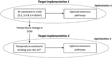
Figure 1. Illustration of the model set-up. Both GET-Climate and DICE-REV are run with implementation approach 1 and implementation approach 2.
Download figure:
Standard image High-resolution imageThe two highest RF2100 targets considered (2.6 W m−2 and 3.4 W m−2) are of central importance in the scenario framework based on the RCPs, the SSPs, and the SPAs (Moss et al 2010, van Vuuren et al 2014, Kriegler et al 2014). This scenario framework was supplemented with an RF target of 1.9 W m−2 to be consistent with 1.5 °C (Rogelj et al 2018b). We find that the temperature ceiling target corresponding to the RF2100 target of 1.9 W m−2 is too stringent in the DICE-REV model (the solver cannot find a solution), and we set a target of 2.2 W m−2 as the most stringent RF2100 target, instead.
For both models we assume that the climate sensitivity is 3 °C per doubling of the CO2-equivalent concentration. This implies that the emission pathways generated by the models would in a probabilistic assessment of climate impacts approximately result in a 50% chance that the temperature in 2100 will be lower than (or equal to) the target set.
A short note on terminology for the sake of clarity when interpreting the results. In this paper we use certain terms as follows.
- Positive emissions: the total CO2 emitted from the combustion of fossil fuels, cement production and net deforestation.
- Negative emissions: all anthropogenic CO2 removal from the atmosphere (e.g. bioenergy with carbon capture and storage; direct air capture).
- Net emissions: the difference between the two (positive emissions less negative emissions)
- Net-negative emissions: net emissions below zero.
It is important to carefully distinguish these emissions concepts. For instance, in certain pathways there may be negative emissions on the order of several GtCO2 per year, but net emissions may nevertheless be positive if negative emissions are lower than positive emissions.
Even though we include all main GHG emissions in the models used in this paper, our analysis focuses on CO2 emissions since they are the only component that goes negative. Finally, all data presented and analysed refer to global emissions.
2.1. GET-climate
GET-Climate is based on a fusion of the technology-oriented global energy system model GET and a simple climate model (Azar et al 2013). The two models are hard-linked, which enables the generation of internally consistent least-cost mitigation pathways for a given climate target (e.g. on temperature, RF or cumulative CO2 emissions) based on a perfect foresight approach. Key greenhouse gases and aerosols are included in the model. Emissions of CO2 (from fossil fuels), CH4 and N2O are modelled endogenously for all anthropogenic sources (see below for more details), while land-use-related CO2 emissions and other forcers (such as HFCs and aerosols) are exogenous, see Azar et al (2013) for more information.
The energy module of GET-Climate includes resource and extraction cost estimates on uranium, oil, natural gas and coal as well as the energy efficiencies and costs of converting them to various energy carriers (Azar et al 2013). Emission factors for coal, oil, and natural gas are applied to estimate energy- and feedstock-related CO2 emissions. Further, supply potentials and costs of renewable energy resources (hydro, wind, solar and biomass) are also considered. Five end-use demand sectors are included: residential and commercial heat, industrial feedstock, industrial heat, electricity and transport (Hedenus et al 2010, Azar et al 2013). Demand is exogenous and is based on an SRES B2 scenario (Azar et al 2013), similar to the 'middle of the road' SSP2.
The cost and potential for wind and solar energy are updated, based on Lehtveer et al (2017), to capture the rapid decline in these costs in recent years. The use of intermittent electricity production is constrained to at most 40% of annual electricity generation (30% in Azar et al (2013), update based on Lehtveer et al (2017)). However, even more intermittent production is allowed if electricity storage technologies are used, which in turn comes at a cost and an efficiency loss. In comparison to Azar et al (2013), the maximum wind power potential has been increased from 40 to 80 EJ per year based on Lehtveer (2017), and nuclear power generation is constrained to at most 15% of electricity supply, instead of 10 EJ per year as in Azar et al (2013), in order to generate model output on par with other IAMs (Huppmann et al 2018). We acknowledge that technology costs are declining rapidly, but the primary focus of this paper is to compare the consequences of different target implementations.
The energy system module in GET-Climate is basically a linear programming model. For the model to generate plausible solutions for the growth of new technologies, limits on expansion rates are used (Wilson et al 2013). These constraints were relatively conservative in the GET-Climate version used in Azar et al (2013) and have now been relaxed. The maximum annual growth rate for the capacity of a specific technology is increased from 15% per year to 20% per year. In addition to maximum growth rates in relative terms, which limits the expansion of technologies with a relatively small market share, we include absolute constraints on yearly expansion, which limits the yearly expansion once a technology has become more mature, see Azar et al (2003, 2006). For the majority of runs and technologies, these constraints are not binding. These assumptions together generate results broadly consistent with output generated by other IAMs and with historical estimates for related technologies (Wilson et al 2013, Huppmann et al 2018).
GET-climate includes negative CO2 emissions using bioenergy with carbon capture and storage (BECCS), assuming standard estimates of global bioenergy availability (a maximum of 200 EJ per year in line with Chum et al (2011)), carbon storage capacity (2000 GtCO2), and climate sensitivity (3 °C per doubling of CO2 concentration) (Azar et al 2013). The discount rate is 5% per year.
Land-use-related CO2 emissions are exogenous and are assumed to decline over time and be net zero from 2080 and onwards, see figure SM 2 (available online at stacks.iop.org/ERL/15/124024/mmedia). This implies relatively high future land-use-related emissions compared to other pathways consistent with low stabilisation targets (Huppman et al 2018).
Reference emissions of CH4 from the extraction of fossil fuels are determined endogenously based on coal mining and extraction of oil and natural gas in the energy system module. N2O emissions as a result of bioenergy production are also determined endogenously based on bioenergy supply. Other CH4 and N2O emissions are based on baseline projections (SRES B2) together with the assumption that emissions can be reduced at a cost determined by abatement cost functions (Azar et al 2013). Other non-CO2 forcers (aerosols, F-gases, CFC, land-use albedo, etc) are based on RCP 2.6 (Meinshausen et al 2011).
We do not use any metrics like Global Warming Potential (GWP) to convert the emissions of non-CO2 forcers to CO2-equivalents, but let the model decide based on the atmospheric lifetime of the gases, their RF impact and the cost of abatement to what extent it is cost-effective to reduce the emissions of each gas, in line with Manne and Richels (2001) and Johansson et al (2006).
The carbon cycle is represented with the non-linear impulse-response model taken from Joos et al (1996), with climate feedbacks based on (Joos et al 2001, Friedlingstein et al 2006). The atmospheric gas dynamics for N2O and CH4 are based on a simple difference equation, where the feedback of CH4 on its own lifetime through depletion of the hydroxyl radical (OH) (Prather et al 2001) is taken into account. RF is estimated based on simple parametric equations (Ramaswamy et al 2001). The indirect effects of CH4 on tropospheric O3 and stratospheric H2O are taken into account following Wigley et al (2002). The resulting global mean surface temperature is estimated with an Upwelling-Diffusion Energy Balance Model (UDEBM) (Azar et al 2013, Sterner et al 2014, Johansson et al 2015).
2.2. DICE-REV
We use version 2016R2 of the DICE model (Nordhaus 2018a) with an updated and recalibrated climate module. DICE is based on an integrated macroeconomic Ramsey growth model, a simple climate model, and estimates of the costs of reducing anthropogenic emissions of CO2 as well as estimates of the damages of climate changes. In the model, net present welfare is calculated based on a constant relative risk aversion utility function. Total consumption equals the total annual global economic output less investment in new capital, cost of abatement, and damages due to climate change. In our model runs, however, we have turned off the damage part in order to show clear results on how the climate target formulation affects the CO2 emission pathways without interaction with the damage function. The general DICE model is explained in detail in Nordhaus (2018a); Nordhaus (2018b)), and the details of the differences between DICE and DICE-REV are described in Hänsel et al (2020).
The model is updated in several ways. First, the carbon cycle is based on the simple climate model FAIR (Millar et al 2017, Smith et al 2018). This carbon cycle representation considers the non-linearities in the carbon cycle as well as climate carbon cycle feedbacks by using a non-linear impulse-response function. The decay time constants of the impulse-response function are dependent on the cumulative uptake of carbon in the ocean and biosphere as well as on the global mean surface temperature change, see Millar et al (2017) for details. Second, the two-box energy balance module in DICE has been recalibrated so that the parameterizations of the effective heat capacities and the heat exchange coefficient generate a step response that corresponds to the average step response of the climate models used in CMIP5 (Geoffroy et al 2013). Further, the climate sensitivity is set to 3.0 °C for a doubling of the atmospheric CO2 concentration (instead of 3.1 °C which is the standard assumption in DICE 2016R2). Third, the exogenous RF pathway for non-CO2 forcers (all non-CO2 GHGs and aerosols) is updated to be roughly halfway between the RCP 2.6 and 4.5 pathways, see figure SM 1.
DICE has no explicit representation of energy technologies or the inertia involved in changing the energy system. The cost of reducing CO2 emissions is based on a marginal abatement cost function, in which the cost increases with increasing relative abatement from the baseline emissions. The exclusion of technology inertia, such as the cost of prematurely retired capital based on fossil fuels, or costs of and constraints on a rapid expansion of carbon-neutral technologies, makes it possible for the model to generate emission pathways that drop (perhaps unrealistically) rapidly over time. Still, the model's simplicity and widespread use, as well as the fact that it contains an integrated temperature response module, make it an appropriate IAM to illustrate how different climate target implementations affect the optimal emission pathway towards the target.
To allow for negative CO2 emissions in DICE-REV, we allow net emissions to go below zero after 2050 instead of after 2160 as is the base case assumption in DICE. As in the standard version of DICE, we stretch the abatement cost function beyond 100% so that the net-negative emissions of CO2 can reach 15% of the baseline emissions from energy and industrial sources. That is, energy and industry CO2 emissions can be reduced by 115% in line with results from many IAMs. The constraints on the timing of when net CO2 emissions may go below zero and the maximum level of net-negative CO2 emissions are based on IAM output included in Huppmann et al (2018) and Rogelj (2018a), see Hänsel et al (2020) for further arguments.
Land-use-related CO2 emissions are exogenous, using the standard assumption in DICE, in which they decline over time by 2.2% per year, see figure SM 2.
2.3. Some limitations of the two IAMs
Both models used for the purpose of this paper have some limitations that should be taken into account when interpreting the results. First, aerosol forcing is exogenous in both models and non-CO2 greenhouse gases are only in part endogenous in GET-Climate (CH4 and N2O are endogenous), while exogenous in DICE-REV. If the link between use of fossil fuels and aerosols were captured and abatement of all major non-CO2 GHGs was endogenous, then this could affect the details of the results. However, CO2 is the main climate forcer, and the emissions of aerosols and aerosol precursors are expected to decline because of policies to control air pollution (Rao et al 2017); this suggests that the effect on the results would not be significant. Further, F-gases are considered cheap to reduce and in a cost-effectiveness framework these would already be reduced to low levels at lower CO2 prices than what we find in our models (Purohit and Höglund-Isaksson 2017). We also run GET-climate with both exogenous and endogenous CH4 and N2O emissions to test the robustness of the results (see section 3.3 and SM 8).
Further, land use is fixed in the models, and there is an exogenously fixed limit on biomass supply in GET-Climate (there are no explicit technologies and thus no explicit biomass supply in DICE-REV). How the future interaction between biomass demand and protection of forest will evolve is impossible to predict. The methodological approach used here is based on an assessment of how much biomass may be supplied sustainably (Chum et al 2011). There are large uncertainties associated with this assumption and although a thorough assessment of the biomass supply potential is beyond the scope of this paper, we assess how the CO2 emission pathways in GET-Climate are affected by alternative assumptions on biomass supply.
Given the limitations mentioned here and the sensitivity analyses performed, we believe that the key insights presented are robust and useful, but as with all model-based studies the insights need to be corroborated by further research.
3. Results
3.1. GET-climate
3.1.1. Net CO2 emission pathways
We first run the GET-Climate model for three RF targets in the year 2100 (RF2100). The resulting emissions and temperature pathways are shown in figure 2. The resulting temperature level in 2100 is then used to rerun the model without allowing the temperature to exceed that level over the entire 21st century (temperature ceiling), thus avoiding temperature overshoot.
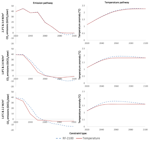
Figure 2. CO2 emission pathways (left) and corresponding global mean temperature increase (right) generated by GET-Climate for three radiative forcing targets (3.4 W m−2, 2.6 W m−2 & 2.2 W m−2) and their implied temperature stabilisation targets (2.3 °C, 1.8 °C, 1.6 °C).
Download figure:
Standard image High-resolution imageThe RF2100 targets of 2.2 W m−2, 2.6 W m−2, and 3.4 W m−2 are calculated to have a temperature increase of, respectively, 1.6 °C, 1.8 °C, and 2.3 °C above pre-industrial levels by the year 2100; these increases are then set as temperature ceiling targets. The temperature peaks during the 21st century and drops towards 2100 for the RF2100 targets, but not for the temperature ceiling targets. However, for the 3.4 W m−2 target, the temperature overshoot during the 21st century is negligible, and the transient difference in surface temperature change between the RF2100 case and the temperature ceiling case is very small.
The way the constraint is implemented (RF2100 or temperature ceiling) has a significant impact on the CO2 emission pathways (figure 2). The difference is greater the more stringent the target. For the 2.2 W m−2 RF2100 target, the cumulative net-negative CO2 emissions are 400 GtCO2 but only 170 GtCO2 for the corresponding 1.6 °C ceiling target, see table 1. For the 2.6 W m−2 RF2100 target, the cumulative net-negative CO2 emissions are 240 GtCO2 and only 80 GtCO2 for the 1.8 °C ceiling target. The cumulative net-negative CO2 emissions are 50 GtCO2 and 10 GtCO2 for the 3.4 W m−2 RF2100 target and the 2.3 °C ceiling target, respectively.
Table 1. Cumulative net emissions, positive emissions, and negative emissions over the period 2020–2100 generated in the IAM GET-Climate for different implementations of climate stabilization constraints. Three radiative forcing targets (3.4 W m−2, 2.6 W m−2, and 2.2 W m−2) are analysed, along with the three corresponding temperature ceilings (2.3 °C, 1.8 °C, and 1.6 °C).
| Pathway name | Cumulative net CO2 emissions 2020–2100 (GtCO2) | Cumulative net-negative CO2 emissions 2020–2100 (GtCO2) | Cumulative positive CO2 emissions 2020–2100 (GtCO2) | Cumulative negative CO2 emissions 2020–2100 (GtCO2) |
|---|---|---|---|---|
| 2.2 W m−2 in 2100 | 420 | 400 | 1430 | 1010 |
| 1.6 °C ceiling target | 450 | 170 | 1430 | 980 |
| Difference | 30 | −230 | 0 | −30 |
| 2.6 W m−2 in 2100 | 800 | 240 | 1600 | 810 |
| 1.8 °C ceiling target | 860 | 80 | 1660 | 800 |
| Difference | 60 | −160 | 60 | −10 |
| 3.4 W m−2 in 2100 | 1670 | 50 | 2200 | 530 |
| 2.3 °C ceiling target | 1700 | 10 | 2190 | 490 |
| Difference | 30 | −40 | −10 | −40 |
The difference in CO2 emission pathways is in part due to abatement costs being discounted. In the model, discounting provides an incentive to postpone abatement. Since the ceiling target implies a more stringent constraint in the near term (and all the way up to the year 2100), abatement will initially be larger with a temperature ceiling constraint than with a RF2100 constraint. The costs and shadow prices for the different targets are discussed in section 3.3.2 and SM 9, 10 & 11, and section SM6 discusses in more detail how the discount rate affects the optimal path under the two types of target formulations.
A second, but much smaller, reason for the difference in CO2 emission pathways is the inertia in the climate system. A pulse emission of CO2 yields an approximately stepwise temperature response (Azar and Johansson 2012, Ricke and Caldeira 2014), leading to the close-to-linear relationship between temperature and cumulative CO2 emissions. However, the maximum RF impact from a CO2 emission pulse occurs at the same time as the emission pulse and decays thereafter. For present concentration levels, roughly 40% of the initial impact remains after 100 years (Azar and Johansson 2012, Joos et al 2013). Hence, the temperature response is dampened relative to the RF response since there is an initial large ocean heat uptake, which subsequently diminishes over time (Solomon et al 2010). Because of this, emitting 1 tonne of CO2 now requires removing 1 tonne CO2 later to get close to zero net temperature change impact; it is basically a one-to-one relationship. However, emitting 1 tonne CO2 now requires removing only about 0.4 tonne CO2 in 2100 to get a close to net zero radiative forcing impact, since the RF response decays over time. This gives an additional incentive to postpone emissions reductions in the RF2100 case.
A third mechanism behind the difference in emission paths has to do with the trade-off between CO2 and non-CO2 greenhouse gas emissions. Given that a pulse emission of CO2 yields an approximately stepwise temperature response (Azar & Johanssn, 2012, Ricke and Caldeira 2014), one may conclude that once global CO2 emissions have reached zero, temperatures will stabilise (in a decade or so) and then remain roughly constant (Matthews and Caldeira 2008, Jones, 2019). It might thus be surprising that our results in figure 2 show net-negative emissions for the temperature ceiling case. The reason is that the net-negative emissions offset the warming effect of a flat or increasing non-CO2 GHG forcing trajectory (SM 5). Hence, the net-negative emissions are the result of a trade-off between abatement of non-CO2 GHG and net-negative CO2 emissions, suggesting that more net-negative CO2 emissions allow for higher CH4 and N2O emissions (cf Peters 2018).
The net CO2 emission pathways generated by GET-Climate are further analyzed for other discount rates and maximum annual bioenergy supply in SM 6 and SM7, respectively. Largely, the difference in net CO2 emission pathways between the two target types increases with increasing discount rate and with increasing bioenergy availability.
3.1.2. Positive and negative CO2 emission pathways
The previous section discussed annual net emissions compatible with a specific climate target. We find that the cumulative net CO2 emissions over the period 2020–2100 are approximately the same for each target pair (see table 1). This is in line with Tokarska et al (2019) who found that the cumulative emissions for a specific temperature anomaly in 2100 are independent of whether the pathway includes overshoot or not. However, as discussed in the previous section, the cumulative net-negative emissions differ depending on the way the climate constraint is implemented (table 1). Despite this, we also find that the cumulative positive emissions and negative emissions (carbon dioxide removal) over the period 2020–2100 are all relatively similar for a given target pair (table 1).
Even though the positive and negative cumulative emissions are similar (table 1), they are distributed differently over time depending on the climate target formulation (figure 3). The more stringent the target, the earlier negative emissions (through BECCS) are generated by GET-Climate, regardless of whether the target is implemented as an RF target or a temperature ceiling target (figure 3). The timing of the positive emissions differs within each target pair, with positive emissions reduced more rapidly in the initial decades with a temperature ceiling, but with higher positive emissions in the second half of the century, resulting in similar cumulative positive emissions for the target pairs. Consequently, in GET-Climate, the temperature ceiling achieves its more limited net-negative emissions by having higher positive emissions, not less negative emissions.

Figure 3. Positive, negative, and net CO2 emission pathways generated in the IAM GET-Climate for the three radiative forcing targets (3.4 W m−2, 2.6 W m−2, and 2.1 W m−2 by the year 2100) and the three corresponding temperature ceilings (2.3 °C, 1.8 °C, and 1.6 °C).
Download figure:
Standard image High-resolution imageAdditional results on primary energy supply in GET-Climate are available in SM 3, and disaggregated results on biomass use can be found in SM 4.
3.2. DICE-REV
3.2.1. Global net CO2 emission pathways
We now present results with the DICE-REV model. The RF2100 targets of 3.4 W m−2, 2.6 W m−2 and 2.2 W m−2 generate temperature pathways that peak during the 21st century and then drop towards 2.1 °C, 1.7 °C and 1.5 °C, respectively, in 2100 (figure 4). The temperature levels in 2100 obtained with DICE-REV are lower than those obtained with GET-Climate (about 0.13 °C), while the temperatures in 2020 are slightly higher (about 0.15 °C). The reasons for these differences are described in section SM 5. By construction, a peak and decline in temperature is not allowed with the temperature ceilings.

Figure 4. CO2 emission pathways and corresponding global mean temperature impacts generated in the IAM DICE-REV for different implementations of climate stabilization constraints. Three radiative forcing targets (3.4 W m−2, 2.6 W m−2, and 2.2 W m−2) are analysed, along with the three corresponding temperature ceilings (2.1 °C, 1.7 °C, and 1.5 °C).
Download figure:
Standard image High-resolution imageSimilar to GET-Climate, the way the climate target is implemented in DICE-REV has a significant impact on the CO2 emission pathway and the amount of net-negative emissions during the second half of the 21st century (figure 4). That there are less net-negative emissions with a temperature ceiling than with the corresponding RF target is even more pronounced in DICE-REV, which only generates very small amounts of net-negative emissions with the temperature ceilings. The models differ because of the interplay between CO2 and non-CO2 GHG emissions (see the discussion in the final paragraph in section 3.1.1), with DICE-REV having lower non-CO2 RF in 2100.
Further, net-negative CO2 emissions are obtained for all three RF overshoot cases. The difference in cumulative net-negative CO2 emissions between the two climate constraint implementations (i.e. RF2100 vs temperature ceiling) increases with increasing constraint stringency. It is not possible to separate the positive and negative emissions in DICE-REV, as only net emissions are modelled.
3.3. Further assessment of pathways in GET-Climate and DICE-REV
3.3.1. Cumulative emissions
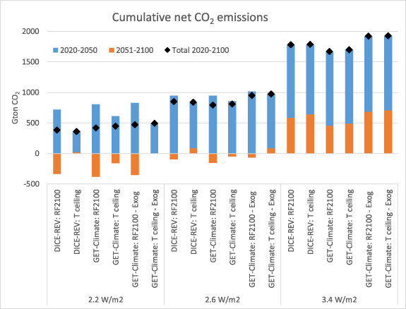
The net CO2 emission pathways generated by GET-Climate and DICE-REV share many features. If we define near-term to be the period 2020–2050 and long-term to be the period 2051–2100, we can readily observe that for the two most stringent pairs of targets, and for both models, the cumulative net CO2 emissions in the near-term are significantly higher and cumulative net CO2 emissions in the long-term are significantly lower (or in some cases more negative) when implementing the target as an RF2100 target as compared to a temperature ceiling (figure 5). Further, the cumulative net CO2 emissions over the whole period 2020–2100 are roughly similar for each target pair, each model, and each assumption on the non-CO2 RF pathway. However, there are some differences between the models and the different assumptions on the non-CO2 RF pathway.
Figure 5. Cumulative net CO2 emissions in GET-Climate and DICE-REV during the time periods, 2020–2050, 2051–2100, and 2020–2100 for the different climate constraint implementations. The term 'Exog' refers to exogenous CH4 and N2O emissions.
Download figure:
Standard image High-resolution image
To further elucidate the differences between the results obtained with the two models, we ran GET-Climate with the same non-CO2 forcing assumption as in DICE-REV (i.e. in this experiment, all forcing agents except CO2 are exogenous in GET-Climate as well). This exogenous RF trajectory is lower than the forcing obtained in the endogenous cases except for a transition period in the 1.6 K temperature ceiling case (see SM 5). The lower non-CO2 RF implies that annual CO2 emissions become slightly higher in all cases except for a few decades for the most stringent temperature ceiling case (see figure SM 12 and table SM 1).
Two main observations are worth mentioning. First, we observe (figure 5) that DICE-REV has smaller cumulative emissions over the period 2020–2100 than what GET-Climate has with the exogenous non-CO2 forcing assumption. This is due to some differences in the way the carbon cycle is implemented in the two models. All else equal, the net uptake of carbon in the biosphere and in the oceans is smaller in the carbon cycle used in DICE-REV than in GET-Climate. Second, under the assumption of the (lower) exogenous forcing for non-CO2 emissions, the amount of net-negative emissions drops to almost negligible levels in GET-Climate as well (see figure SM 12 right panel, table SM 1, and also figure 5).
The output from GET-Climate with endogenous non-CO2 forcing and DICE-REV is further compared in section SM 5. Also, to corroborate the validity of the climate modules in GET-Climate and DICE-REV, the emission pathways generated by the models are analyzed in MAGICC 6.0 (Meinshausen et al 2011), see SM 12.
3.3.2. Abatement costs
The abatement costs to meet the different climate targets are shown in table 2. We find that abatement costs are higher with temperature ceilings than with the RF2100 constraints. The reason for the higher cost is that more near-term abatement is required in the temperature ceiling cases, and this dominates the smaller abatement during subsequent periods given the discount rates used (5% per year in GET climate and around 5% per year in DICE-REV). Annual abatement costs are presented in SM 11, and shadow prices on emissions in SM 7 and 8.
Table 2. Net Present Value (NPV) of future abatement cost in per cent of NPV future GDP.
| Target level | Target approach | GET-Climate | DICE-REV |
|---|---|---|---|
| 2.2 W m−2 in 2100 | RF2100 | 1.54% | 2.11% |
| Temperature ceiling | 1.64% | 2.83% | |
| 2.6 W m−2 in 2100 | RF2100 | 0.88% | 1.43% |
| Temperature ceiling | 1.06% | 1.68% | |
| 3.4 W m−2 in 2100 | RF2100 | 0.45% | 0.68% |
| Temperature ceiling | 0.57% | 0.70% |
However, note that the transient temperature response during the 21st century is higher in the RF2100 target cases because of the peak and decline in temperature (see figures 2 and 4) and that the costs of the associated climate damages have not been included in these calculations.
4. Discussion
Most scenarios with stringent climate targets result in large net-negative CO2 emissions towards the end of the century (Azar et al 2006, Andersson & Peters, 2017, van Vuuren et al 2017, Bauer et al 2018, Rogelj et al 2018a). This has spurred discussions about the role of carbon removal technologies, particularly BECCS. In this paper, we show that the amount of net-negative emissions strongly depends on how the climate constraint is implemented in the model. We run two different IAMs, GET-Climate and a revised version of DICE, here called DICE-REV, with the climate constraint implemented either as an RF target reached by the year 2100 or as a temperature ceiling over the 21st century.
We find that pathways generated under an RF2100 target have higher CO2 emissions in the near term and greater net-negative CO2 emissions towards the end of the century compared to pathways obtained under a temperature ceiling. This holds in both models. The difference in emission pathways for the two implementations increases with increasing stringency of the climate constraint.
When running GET-Climate with endogenous abatement of CH4 and N2O, some net-negative emissions remain towards the end of the century even with a temperature ceiling. In a hypothetical case, where there are no non-CO2 greenhouse gases involved, this result should not be expected, as net-zero CO2 emissions lead to a roughly constant temperature, and hence net-negative CO2 emissions would lead to a decrease in temperature. However, with other GHGs involved and a temperature ceiling, net-negative CO2 emissions result from an economic trade-off between non-CO2 GHG emissions and negative emissions in GET-Climate. The model essentially finds it more cost effective to allow for higher emissions of CH4 and N2O and compensate for this by letting global emissions of CO2 drop to below zero. Thus, the interplay with non-CO2 GHG emissions could play an important role in determining the amount of (net) negative emissions achieved in a model run. When running DICE-REV and GET-Climate with the same exogenous non-CO2 RF assumptions, there are, with a temperature ceiling, hardly any net-negative emissions (figure 4, figure SM 8 and table SM 1). This is in line with expectations of no or only little temperature change with net-zero CO2 emissions.
Our results imply that the climate target formulation has significant impacts on both near-term and long-term emission pathways towards the target and on the perceived need for net-negative emissions. variety of target implementations when running IAMs against a given climate target to avoid presenting a biased message on the role of net-negative CO2 emissions for stringent climate targets. Further, non-CO2 GHG emissions may also play an important role when it comes to determining the level of net-negative CO2 emissions, and this requires further investigation across a range of models.
Although we find limited use of net-negative emissions in meeting temperature ceiling targets, we nonetheless find that large amounts of negative emissions are cost-effective in all our GET-Climate runs. In these scenarios, negative emissions are used to compensate for emissions (including non-CO2 emissions) in sectors where 100% mitigation is difficult or costly (see also Luderer et al 2018). Interestingly, the amount of cumulative negative emissions (i.e. cumulative gross CO2 removals) are about the same regardless of the type of climate target formulation (table 1). In the sensitivity analysis, we find this result to hold in most other runs, but in a case with a 50% higher supply of biomass, negative emissions tend to be somewhat higher in the RF2100 case than in the temperature ceiling case towards the end of the century.
The results presented here show the outcome of two IAMs that assume full cooperation among nations to reduce emissions of greenhouse gases at the lowest possible cost. The pathways should thus be seen as illustrative of how the target formulations affect IAM-generated emission trajectories as well as the scale of net-negative emissions towards the end of the century, but not necessarily as politically achievable or desirable emission pathways to stabilise climate.
In the real world, meeting the 1.5 °C or 2 °C target is extremely challenging (Jewell and Cherp 2020). If we fail to rapidly reduce emissions of CO2 and other GHGs in the near term, an overshoot above the long-term targeted temperature stabilisation level is likely to be unavoidable. Net-negative CO2 emissions are then necessary in order to reduce the global mean surface temperature if society is to meet stringent stabilisation levels consistent with the Paris Agreement (Azar et al 2013).
4.1. Comparison with recent literature
In a recent paper, Rogelj et al (2019) presented an alternative approach to constructing emission scenarios using IAMs. Our motivation here is similar to theirs. Their approach is based on cumulative emissions targets up to the time of net-zero emissions and then exogenously set annual emissions targets in 2100 to generate a stable or declining temperature. Such a scenario construction could avoid (large) temperature overshoots that often result when optimizing towards RF targets in 2100.
One possible concern with the approach suggested by Rogelj et al (2019) is that it leads to emission pathways that are largely determined exogenously and ex ante instead of optimised over time for a given climate target level. They require specifying three parameters to constrain the temperature (peak temperature, peak year, and annual net-negative emissions), as opposed to just applying a temperature target. The strong ex-ante assumptions on timing would limit the usefulness of intertemporal optimization models, since they are in large part designed to study optimal pathways and trade-offs over time.
This challenge spills over onto how to deal with non-CO2 emissions. Rogelj et al (2019) suggest an iterative approach where shadow prices of CO2 are first estimated in an optimisation with constraints on cumulative emissions followed by annual emissions. Abatement of non-CO2 GHG emissions are estimated ex post using those shadow prices on CO2 and the GWP to weight different GHGs.
Both the approach analysed by Rogelj et al (2019) and the one analysed in this study have strengths and weaknesses. Optimizing towards a temperature target is relatively convenient, while the approach suggested in Rogelj et al (2019) would involve several model iterations if a specific temperature level were to be achieved. On the other hand, our inclusion of a hard-linked climate model increases model solution times and makes the optimization problem harder due to (additional) non-linearities. Optimizing towards a temperature target is consistent with an approach where the temporal dynamics of the different GHGs are considered in the optimization (Manne and Richels 2001, Johansson et al 2006, Johansson 2012), while the approach suggested by Rogelj et al (2019) fits better if one wants to use a certain metric such as GWP. Hence, our different approaches could be seen as complementary and will generate relatively consistent results if they are set to meet (close to) equivalent targets (e.g. temperature ceilings).
5. Conclusion
We have analysed the role of gross and net-negative CO2 emissions in scenarios towards stringent climate constraints. In most previous studies, significant amounts of net-negative emissions at the global scale feature prominently. Here we have shown that this is to a large extent the result of how the climate target is implemented in the IAMs.
We use two different types of climate targets with each of two different IAMs: a temperature ceiling (implemented as a ceiling over the 21st century and beyond) and an RF target by the year 2100 and beyond (as this is the climate target assessed by most IAMs). We find that the net-negative CO2 emissions tend to be significantly lower (or non-existent) when running the models with a temperature ceiling than with a RF target in 2100. This also implies that temperature ceilings result in emission pathways in the near term that are significantly lower than for the corresponding RF overshoot targets. We analyse temperature ceilings as low as about 1.6 °C above the pre-industrial level. However, more stringent targets than that are likely to require, even from a purely technical perspective, a temporary overshoot in the temperature given the proximity to the target.
Further, we also find using GET-Climate that cumulative net CO2 emissions, cumulative positive CO2 emissions, and cumulative negative CO2 emissions (cumulative gross CO2 removals) are all about the same for each target pair for our base case assumptions. Even though the amount of net-negative emissions strongly depends on the type of climate target formulation, this does not necessarily hold for the overall use of negative emissions. Largely, this is because negative emissions through BECCS are likely to be a relatively low-cost abatement option for deep CO2 emission cuts if constraints on biomass are not a key issue. Furthermore, a temperature ceiling, which involves more rapid emission reductions, generates a larger NPV abatement cost than a comparable RF target in 2100.
Finally, we argue that to avoid presenting a biased message on emission pathways and the role of net-negative CO2 emissions, it is important to use a diversity of climate target formulations when generating emission pathways in IAMs, as each method has its drawbacks, and consequently to soften the prevailing focus on RF levels in 2100.
Acknowledgments
We thank Sabine Fuss for valuable comments and Paulina Essunger for proofreading. Christian Azar was supported by the Carl Bennet AB Foundation, Daniel Johansson was supported by Mistra through the project Mistra Carbon Exit, while Glen Peters was supported by the European Commission Horizon 2020 project Paris Reinforce (Grant No. 820846).
Data availability statement
The data that support the findings of this study are available upon reasonable request from the authors.