


Abstract
Global flood models (GFMs) and earth observation (EO) play a crucial role in characterising flooding, especially in data-sparse, under-resourced regions of the world. However, validation studies are often limited to a handful of historic events and do not directly assess the ability of these products to simulate flood hazard—the probability that flooding will occur in a given location. As a result, it is difficult for stakeholders to decipher the ability of either models or observations to identify flood hazard and make decisions to mitigate for flooding. Here, we leverage flood observations from 20 years of MODIS data to compare the recorded flooding with what would be expected given the hazard simulated by a GFM. We devise an approach, Flood Expectation Per Pixel, and apply it across four large basins in Africa—Congo, Niger, Nile and Volta representing a variety of biomes. We estimate the uncertainty of EO to capture flood events due to burned areas, cloud cover and vegetation, incorporating uncertainty estimates when comparing to modelled hazard. We found that at lower return periods (RPs) (<20 years), the EO data records less flooding than the GFM, suggesting GFMs overpredict frequent flooding. For RPs between 50 and 100 years, GFM and EO data show greater consistency given the uncertainties we consider. For large RPs (100 years) the EO observations show more flooding than expected given the GFM data, potentially due to data errors and non-fluvial flooding, however there are too few observations to draw significant conclusions at these RPs. The EO record indicates that the GFM can differentiate between flood RPs. We find EO and GFM complement each other and thus should be used in tandem to inform strategies to mitigate floods across the hazard spectrum from frequent to extreme flood events.
Export citation and abstract BibTeX RIS

Original content from this work may be used under the terms of the Creative Commons Attribution 4.0 license. Any further distribution of this work must maintain attribution to the author(s) and the title of the work, journal citation and DOI.
1. Introduction
Flooding is the most frequent and deadliest natural hazard, causing billions of dollars in annual damages globally (Berz et al 2001, MUNICHRE 2020). Estimating where flooding might occur is of crucial importance to making informed risk management decisions to prevent fatalities and reduce loss of assets. Fatalities from flooding are disproportionally high in developing countries (Jongman et al 2012), where data regarding flood risk is the most inadequate. Flood impacts are expected to increase due to expanding populations in floodplains (Changnon et al 2000, Winsemius et al 2016, Wing et al 2018), climatic changes (Alfieri et al 2017, Ward et al 2014, Arnell and Gosling 2016), and increased risk from compound events (Zscheischler et al 2018). Hydrodynamic models and Earth Observations (EOs) can and are increasingly used to characterise past, present and future flooding. Yet the validation of flood models are often limited to single events and individual case studies, making it difficult for decision-makers to decipher the ability of either models or remotely sensed flood data to inform decisions. Here we compare how hydrodynamic models and EO products charactise flood hazard, to provide guidance for stakeholders to use these tools appropriately to increase flood resilience and reduce flood risk.
Hydrodynamic models take information about discharge, topography and river geometry to simulate inundation. These models usually produce hazard estimates, which map the probability of flooding exceeding a particular depth or extent in terms of annual exceedance probability (AEP) or its inverse a return period (RP). Global Flood Models (GFMs) can provide this hazard information globally (Yamazaki et al 2011, Pappenberger et al 2012, Sampson et al 2015, Dottori et al 2016) and are increasingly being used in disaster management (Ward et al 2014, the WRI Aqueduct model, based on Winsemius et al (2013)) and to assess flood risks under changing climates (Hirabayashi et al 2013, Winsemius et al 2016).
Despite the scientific rigour and expense dedicated to developing global hazard products, there are surprisingly few validation studies and model evaluations relevant to this scale of modelling. GFM intercomparison studies at large scales have revealed substantial disagreement among models (Sampson et al 2015, Trigg et al 2016, Wing et al 2017, Aerts et al 2020). Moreover, studies that compare modelled flooded area to observations are much more common at the reach scale and usually take simulations of a single (often large) flood event and compare this to independent observations from EO (Horritt and Bates 2002, Bates et al 2006, Schumann et al 2013, Dottori et al 2016) wrack marks/water level (Neal et al 2009, Lhomme et al 2010), reports of fatalities and/or financial losses (Zischg et al 2018) or another hydrodynamic model (Hoch et al 2017, Wing et al 2017, Fleischmann et al 2019). These event-based approaches remain popular due to inadequate validation data with large spatial and temporal coverage (Molinari et al 2019). However, the event-based studies and model intercomparison undertaken to date have yet to effectively evaluate or validate GFM skill to identify flood hazard across a spectrum of frequencies.
The proliferation of EO data and significant advances in cloud computing over the last decade have made inundation mapping possible over increasingly larger scales. Algorithms to produce flood maps of inundation extent from satellites are now commonly produced by universities, space agencies, and companies for disaster recovery and response (Policelli et al 2016, Alfieri et al 2018, Schumann et al 2018, Shen et al 2019, Bonafilia et al 2020, Devries et al 2020). Historically, flood maps have been generated for discrete events, however increased computing power, length of the satellite record, and type of satellite sensors has enabled global scale continuous observations of surface water at daily and monthly time steps at various resolutions (Klein et al 2015, Pekel et al 2016, Ji et al 2018). Stakeholders have begun to use flood frequency observations to identify refugee camps at risk at relocate them (Zajic 2019). However, similar to the validation challenges faced by GFMs, no studies, to our knowledge, exist to evaluate the skill of EO to identify flood frequency.
This study provides a novel contribution by comparing flooding observed by satellites with hazard estimates from hydrodynamic models. The objective of this paper is to ascertain consistency (and conversely inconsistency) between hydrodynamic modeling and remotely sensed observation to inform flood hazard. Thus, we intercompare how models and EO observations represent flood hazard across multiple RPs, from frequent (5 year RP) to rarer events (100 year RP). We develop an approach called flood expectation per pixel (FEPP) to meet this objective and compare the full 20-year record of MODIS observations to a widely employed GFM over four large river basins in Africa. Our approach aims to help users of flood hazards and EO products to better understand how and when to use GFMs and EOs of flood hazards to inform decision making to increase flood resilience and mitigate risk.
2. Materials and methods
Here we outline the study sites, GFM and EO data set and introduce our novel method, FEPP, used to intercompare flood hazard estimates.
2.1. Study sites
We focus our analysis in Sub-Saharan Africa, a region of the world where flood risk is expected to increase in the future, yet where arguably the largest gaps in understanding flood risk remain (Tschakert et al 2010). Recent flood events such as cyclones Idai and Kenneth in south-east Africa (Spring 2019), flooding in DR Congo and Republic of Congo (Nov 2019), and South Sudan (July 2019), have highlighted the devastating impact flooding can have on vulnerable populations in Africa and elsewhere. Future percentage increase in population exposed (2010–2050 compared to 1970–2010) to flooding is predicted to be highest globally in North and sub-Saharan Africa (Jongman et al 2012), compounded by intensive and unplanned development into flood-prone zones (Di Baldassarre et al 2010) and an increasingly unpredictable and variable climate (Ficchì and Stephens 2019). Bespoke commercial flood models are often too costly for decision-makers in this region, and calibrating open-source flood models is difficult due to inadequate river-gauge spatio-temporal coverage (Hannah et al 2011, Gleason and Hamdan 2017) or poor topographic data (Shastry et al 2020). Thus, GFMs and satellite information are the most accessible options to inform flood risk decisions. To apply our methodology, we select four hydro-climatologically diverse basins—the Congo; Niger; Nile and Volta basins. These river basins have a combined area of ∼8.2 million km2, or ∼28% of Africa's total land area. The basins also represent a number of known challenges to both EO and GFMs. For instance, the Congo Basin is densely vegetated and has a low number of clear-view (i.e. cloud free) days, which presents a challenge for remotely sensed record (Syvitski et al 2012, Schumann and Moller 2015). Additionally, the Nile Basin is heavily managed for water use (e.g. dams and irrigation), and includes a large delta area, making it difficult to model flood hazard in this basin accurately (Johnston and Smakhtin 2014). These basins also represent a wide range of ecology and biomes, spanning tropical forest to deserts that may have diverse responses to flood hazard models and remote sensing of floods.
2.2. Hydrodynamic model
We use the Fathom GFM (Sampson et al 2015), which simulates riverine flooding globally in 2D at a 3 arc second (∼90 m) resolution for all river basins with an upstream catchment area >50 km2. The modelling framework utilises a sub-grid channel hydrodynamic model within LISFLOOD-FP (Neal et al 2012) to explicitly represent river channels. Boundary conditions for the model are taken from a regionalised flood frequency analysis conducted at a global scale (Smith et al 2015), which links river discharge and rainfall measurements in gauged catchments to ungauged catchments by upstream catchment characteristics and climatological indicators. The version of the GFM used in this study differs from the Sampson et al (2015) version in so far as topography information stems from the MERIT DEM (Yamazaki et al 2017) and the river network from MERIT-Hydro (Yamazaki et al 2019). Thus, the GFM used here may be considered the latest state-of-the-art GFM. Simulations were conducted by RP, with 10 RPs available (5, 10, 20, 50, 75, 100, 200, 250, 500, 1000 years).
2.3. MODIS flood observations
We used the Cloud to Street Flood Recurrence data product, which uses twice-daily MODIS (Moderate Resolution Imaging Spectroradiometer) surface reflectance images to detect surface water fluctuations and recurrence from 2000 to 2019. MODIS provides two daily images of the entire globe from 250-m to 1-km resolution, and is commonly used for flood monitoring including NASA's Near Real Time Global Flood Mapping effort (Xiao et al 2006, Islam et al 2010, Feng et al 2012, Boschetti et al 2014, Klein et al 2015, Ji et al 2018). We apply a modified version of the Brakenridge and Anderson (2006) algorithm (see Tellman et al 2021 for details, summarized here) to map inundation with MODIS using Google Earth Engine (GEE). MODIS Terra (MOD09GA/GQ) and Aqua (MYD09GA/GQ) provide visible, near-infrared (NIR), and short-wave infrared bands (SWIR) important for surface water monitoring. We harmonized the resolution of all bands to 250-m by downscaling the SWIR band from 500-m using corrected reflectance pan-sharpening (Gumley et al 2010). Pixels are then flagged as water or non-water by applying thresholds to three bands: red (b1), SWIR (b7) and a ratio of NIR-red (b2b1ratio). Threshold values are based on Brakenridge and Anderson (2006) who determined values for each band by regressing MODIS reflectance on discharge data. Finally, we use a 3-d composite where a pixel must be classified as water in 4 out of the 6 (i.e. 66%) available images to remain classified to account for cloud and cloud shadow misclassifications. As clouds and cloud shadows move throughout the 3-d composite, overlapping misclassifications of cloud shadows do not occur frequently enough to provide a significantly large number of false positive observations.
Based on this water detection algorithm, annual flood frequency is estimated following the method described in Tellman et al (2021). The daily water detections are combined into annual composites, representing a total maximum annual flood extent and number of per pixel flood detections in each year. To estimate the annual inundation frequency at each pixel, we then divided the number of years a pixel was detected as water by the length of the EO record (i.e. 20 years in the case of MODIS). We refer to this product throughout as observed recurrence. Using an optical sensor for flood monitoring, however, can yield uncertainty of which we have identified three main sources—clouds, fires and vegetation. Floods cannot be detected by satellite when they occur under thick clouds or dense canopies, which could cause false negative in satellite imagery. Fires can reduce reflectance and mimic the low reflectance of water features, causing false positives of flood detection. See supplementary materials (https://stacks.iop.org/ERL/15/124032/mmedia) for further details on these sources of uncertainty.
2.4. Method
To intercompare how the GFM and EO data characterise flood hazard, we developed a novel comparison method that we refer to as FEPP (figure 1). In simple terms, the aim of this method is to convert the hazard simulated by the GFM into the expected number of flooded years that the EO data will see for each pixel. Since many of the RPs simulated by the GFM are longer than the observed record length the expected number of flood observations is often below 1, thus the modelled hazard is comparable to the observed recurrence in the method outlined below only over a very large number of pixels and events from different locations and under the assumption that events are independent.
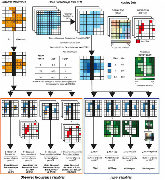
Figure 1. Flood Expectation Per Pixel (FEPP) method overview.
Download figure:
Standard image High-resolution imageFirst the GFM flood hazard maps (all 10 RPs available at ∼90 m resolution) are resampled to the resolution of the observed recurrence data (∼250 m) using bilinear interpolation. We retain only the shortest RP in each pixel resulting in a single raster of RP for the GFM. RP in each pixel is then converted to AEP:
Thus, AEP is the probability of a pixel being flooded in any year according to the GFM. The AEP was then converted to FEPP by multiplying AEP by the length of the observed recurrence record (equation (2))

For completeness, the observed recurrence (number of observed flood years) can also be divided by the length of the record to give annual recurrence (AR), which is directly comparable to the AEP:
Thus, the analysis could be done in terms of AEP or expected number of floods. Here we present in terms of expected number of floods.
The observed recurrence data used in this study has a record length of 20 years. Therefore, for the 5-year RP (AEP = 0.2), we would expect to record a flood 4 times per pixel over a 20-year period (FEPP = 4), or in other words the observed recurrence would on average have a value of four for pixels where AEP = 0.2 if the model is an unbiased reflection of the observed recurrence. For the 20-year RP we would expect to record the flood on average once per pixel in the observed recurrence data. It is unlikely the largest RP used in the is study (100 year) would be detected in the observed recurrence data, and as such the FEPP would be small at a value of 0.2 (AEP of 0.01 × 20 years). See the table in figure 1 for example conversions. Although, it is unlikely to record rare floods in the 20 year EO record used in this study, it is possible. For example, Samimi et al (2012) estimate the 2007 Sahel floods had, in places, RPs of up to 200 years in the Niger and 1200 years in the Upper Volta. Consequently, by converting the AEP from the flood hazard to FEPP we can compare flood hazard at relatively long RPs (in this case up to 1000 years in supplementary materials) with a comparatively short observation record (20 years) provided we have observations from enough distinct flood events from which to calculate an average, which we estimate in section 2.5. (e.g. we are limited to looking at very large catchments or groups of catchments).
It should be noted that in our approach we are comparing two datasets that exhibit different spatial dependence characteristics. Pixels in the observed recurrence data are spatially dependent as observations are based on detecting real flood events in the past 20 years. Pixels in the GFM are spatially independent as river discharge estimates used to force the model are NOT event-based but instead based on a statistical regional flood frequency analysis approach. In other words, the RP of discharge is assumed to be the same (or univariate) across the entire basin in the GFM. Intuitively, we know that real floods are spatially dependent (Keef et al 2012, Quinn et al 2019, Metin et al 2020), especially over large areas. Spatial dependence is affected by spatial-temporal patterns of rainfall (i.e. how large a storm is), land-use and runoff properties, network typology and channel-floodplain hydraulics (Quinn et al 2019). To add spatial dependence to GFM predictions, one could either (1) run a hydrological-hydrodynamic simulation, (2) force the GFM with gauge observations (Schumann et al 2016) or (3) produce a stochastic event set based on gauge observations (Quinn et al 2019). All approaches are computationally expensive and thus impractical at the scale analysed in this paper. While our method compares two different types of data, we justify our approach based on the fact that both datasets are now made readily available to users globally, yet their relative performance for decisions has remained untested.
To focus on flooding we masked out permanent water from both data sets using the G3WBN Version 1.3 water mask (Yamazaki et al 2015). We calculated nine output variables that account for factors we know will influence the detection of flooding—five from observed recurrence and four from the GFM FEPP data.
The observed recurrence variables are: Mean Observed Recurrence per AEP (MOR); Mean Observed Recurrence Burnt per AEP (MORB); Mean Observed Recurrence Burnt Wetland per AEP (MORBW); Mean Observed Recurrence with Clump Sieve per AEP (MORCS) and Mean Observed Recurrence Burnt with Clump Sieve per AEP (MORBCS). To calculate Mean Observed Recurrence per AEP (MOR), we sum the MODIS recurrence pixel values (1–20) for all pixels within a particular GFM AEP and then divide by the total number of pixels in that GFM AEP zone. This gives us average observed recurrence per AEP (or RP) zone, which is comparable with FEPP due to analysing a large number of pixels and events at many locations. Mean Observed Recurrence Burnt per AEP (MORB) is similar but burned areas are masked from the observed recurrence data on a year-by-year basis prior to calculating the average recurrence per AEP. MORBW is similar to MORB, but additionally has wetland pixels (>10 floods in 20 years) removed from the observed recurrence record. We created the MORBW variable as the GFM does not model wetlands, and removing wetlands allows for a more congruent comparison between EO and GFM. MORCS additionally removes isolated pixels from the observed recurrence data, which range in size from a single pixel to blocks of 4 × 4 pixels (∼1 km × ∼1 km). Removal of these small clumps of pixels were designed to remove noise from the observed recurrence data, but as this might also remove small real events all filter sizes are retained to give a range of outputs. MORBCS is similar but has the isolated pixel removal applied to MORB.
We used two resampled auxiliary data sets to condition FEPP based on cloud and vegetation coverage. MODIS is less likely to record flooding when canopy closure is high and we take two approaches to accounting for these unobserved floods. The first considers the inverse of the canopy closure (i.e. 0 = 100% canopy closure; 1 = 0% canopy closure) by multiplying FEPP in each pixel by the inversed fraction vegetation layer for that pixel to calculate the expectation of sensing floods under varying levels of vegetation (FEPPveg). A second method (FEPPveg60) is similar to FEPPveg, but has a binary threshold applied to the vegetation layer where canopy closure ≥60% has a value of 0 and <60% has a value of 1. The threshold of 60% was based upon a histogram of recurrence values against canopy cover for the Congo basin (available in supplementary materials). We further adjust FEPP by considering cloud cover and vegetation in the FEPPvegcloud variable. FEPP will be lower for a short event (often on smaller catchments) and for locations with fewer cloud free observation after large precipitation events because MODIS is less likely to record a flood. Therefore, to calculate FEPPvegcloud, we multiply FEPPveg by the % clear observation value for each day in the 10-d clear day record (outlined in 2.2.1). Finally, the sum of FEPP values for all pixels within each GFM AEP are divided by the total number of pixels within that GFM AEP to get an average for comparison to the observed recurrence averages.
2.5. Detecting the number of flood events
The EO record is relatively short (<20 years), yet the most damaging flood hazards are rare and may not observed in a single basin over that period. We thus trade space for time, by analysing a large area and estimate the likelihood of rare events have indeed occurred over the study regions. We estimate the number of flood events for each basin at each given AEP because we can only expect the FEPP from the GFM and EO record to be comparable when many events have been observed at many locations. On an individual pixel basis, the comparison of FEPP and the EO record makes little sense because the expectation is to see less than one event at pixels where the GFM simulates RPs beyond the record length. Furthermore, if we observe few events in the basin, we will also not expect the EO record and FEPP to be comparable and would need to extend the analysis over a greater number of locations. Flood events are commonly defined using river gauges (Ouarda et al 2006, Bezak et al 2014) or observations of precipitation (Haberlandt et al 2008) in combination with hydrological models (Wu et al 2012). However, given the sparsity of reliable river and rain gauges in our basins, and the unreliability of satellite precipitation products in the region (Cattani et al 2016, Camberlin et al 2019), we chose to use the EO record itself to characterise the number of flood events. To our knowledge there have been no studies in defining flood events using EO flood recurrence data, so here we present a simple method to do so with further details in supplementary materials.
For clarity we briefly outline the five-step method (figure 2). First, each basin was divided into sub-basins. Then the number of flooded pixels detected in the EO data were calculated per sub-basin for event window sizes of 14 and 28 d. Second, in each sub-basin flood peaks were defined from the number of flooded pixels in each event window. Third, we used two clustering algorithms (Hierarchical clustering (HCLUST) and Hierarchical Density-based spatial clustering of applications with noise (HDBSCAN)) to spatially group flooded sub-basins, varying parameters to create 20 estimates of the number of events. Fourth, we summed the total number of events over the EO record and calculated the probability of the number of events for each AEP. Finally, we selected the most probable number of events for each AEP for all 20 clustering variations and present the mean number of flood events we are most likely to have observed in each basin for each AEP assuming the magnitude of each event is independent (figures 3(b)–(e)).
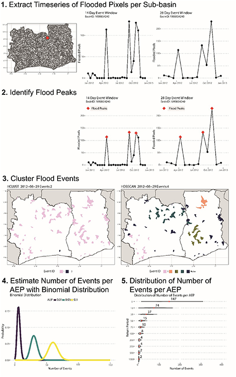
Figure 2. Schematic of the method to estimate the number of flood events seen in the EO record.
Download figure:
Standard image High-resolution image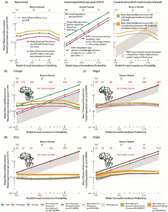
Figure 3. Flood Expectation per pixel (FEPP) for 4 basins (Congo, Niger, Nile and Volta) based on MODIS Annual Recurrence and Fathom Global Flood Model. The y-axis gives the Mean Observed Recurrence/FEPP and the x-axis the Annual Exceedance Probability (AEP) of the GFM (i.e. AEP = 0.01 is a 1 in 100 year return period). (a) Provides a guide how to read the data. b-e are the plots for each basin. The lines show FEPP, FEPPveg60, FEPPveg, Mean Observed Recurrence (MOR), Mean Observed Recurrence with burned areas removed (MORB) and Mean Observed Recurrence with burned areas and wetlands removed (MORBW). The orange shading gives the bounds of Mean Observed Recurrence sums when clumps of 1 pixel to 16 pixels (4 × 4 pixels or 1 km2) are removed (MORCS), while the green shading gives the equivalent for mean observed recurrence with burned areas removed (MORBCS). The grey shading gives FEPPvegcloud which is FEPPveg plus %clear days from 1 to 10 d after the precipitation event. The red numbers are the mean estimated number of events for each AEP.
Download figure:
Standard image High-resolution image3. Results
The nine Recurrence and FEPP variables are plotted in figure 3. Perfect consistency between the GFM and EO data would result in the recurrence lines (pink/green/yellow) matching the FEPP line (turquoise), which, not unsurprisingly, does not occur for any of the basins. Note the mean observed recurrence/FEPP values (y-axis) are on a log scale. Here we present results up to the 100 year flood event, with more extreme events up to the 1000 year flood available in supplementary material. We justify this choice given the high uncertainty in observing the most extreme flood events >0.01 AEP from the 20 year recurrence record. The EO data and the GFM tend to most agree around the 100-year RP, but diverge for both more frequent and less frequent RPs. The EO data observes less flooding than the flood model expects below 20 years, while the EO data tend to identify more flooding than expected on floodplains predicted by the model as being above 250-year RP (see Supplementary materials for AEP > 0.01). At the most frequent (0.2 AEP) and rarest (0.001 AEP) there is approximately an order of magnitude difference between observed recurrence variables and FEPP. The mean estimated number of events for each AEP are given in red in figure 3, with the size of the basin correlating to the estimated number of events (i.e. smallest basin has the fewest events). We can be less confident in our assertions for rarer events, especially for RPs greater than 250 years. The best agreement between GFM and EO data is approximately between 50 and 100 year RP, where we estimate between 12 and 169 events having occurred so can be fairly confident in our results. This agreement may also suggest that a 50–100 year flood event has occurred in the past 20 years. Discrepancies between the FEPP, FEPPveg and FEPPveg60 lines indicate results are affected by vegetation. As would be expected, the Congo basin has the largest discrepancies between the FEPP and FEPP vegetation variations owing to the dense vegetation of the Congo rainforest. The Volta basin also has some discrepancies, while the more arid Nile and Niger basins have very similar FEPP, FEPPveg and FEPPveg60 lines. The grey band (FEPPvegcloud) in figure 3 incorporates cloud cover with FEPPveg. A thicker grey band indicates fewer clear days after a precipitation event, and thus MODIS is less likely to detect flooding. Again, as expected, the Congo has the thickest grey band (so the fewest clear days), while the other three basins have a similar thickness to the grey band so cloud coverage is approximately similar. The orange band is the observed recurrence values where small clumps of pixels are removed, whereas the green band is the same but for observed recurrence with burned areas removed. These clumps range from a single pixel, to blocks of 4 × 4 pixels (∼1 km2). The Volta has a thicker orange and green bands at higher RPs, whilst the other sites have a barely noticeable orange/pink band, indicating the Volta has more instances of isolated flooded pixels in the recurrence record, which could be an indicator of noise in the MODIS data or the presence of many smaller floodplains. Including wetlands in the MORBW variable reduces the Mean Observed recurrence/FEPP value, with the greatest reduction for the larger RP in the Niger which corroborates with the wetland area we find in the EO data that has a large RP in the GFM (figures 5(i) and (j)).
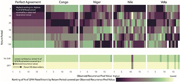
Figure 4. Ranking of % of GFM Flood extent by Return Period covered per Observed Recurrence Pixel Value for each basin. The left hand heatmap indicates an idealised perfect agreement scenario. White indicates no observations. No skill describes the whole basin and Off-Floodplain describes the areas NOT in the GFM flood extents.
Download figure:
Standard image High-resolution imageThe distribution of observed recurrence values for each GFM AEP is graphically represented in the heatmaps of figure 4 by displaying the ranking of % of GFM flood extent by AEP/RP covered per observed recurrence pixel value. If the delineation of the floodplain by RP has skill then more floods per unit area should have been observed for the shorter RP. If each zone of increasing RP floods less often this would result in a dark purple to yellow scale from top to bottom as indicated by the Perfect Agreement heatmap. We also include observed recurrence values that are not in the GFM flood hazard zones in what is called off-the-floodplain (OFP), and a 'no-skill' category which describes recurrence values across all pixels per study site.
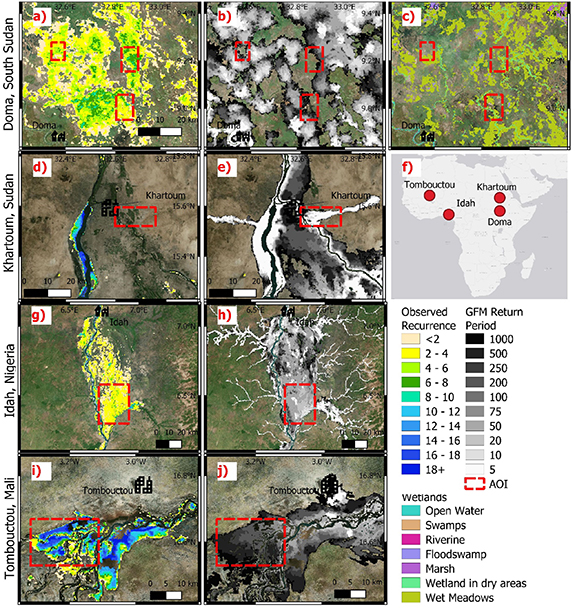
Figure 5. Maps of observed recurrence (a),(d),(g),(i), GFM flood extent by return period (b),(e),(h),(j), Wetlands (c) and a location map (f) for Doma, South Sudan; Khartoum, Sudan; Idah, Nigeria and Tombouctou, Mali.
Download figure:
Standard image High-resolution image
If the models have skill at delineating floodplain from non-floodplain these categories should have the lowest ranked recurrence. The purpose of figure 4 is to determine whether the GFM and EO record taken together can differentiate between flood hazard severity (i.e. RPs). We can be more confident of making conclusions based on the smaller recurrence values as there are more observations, and thus the x-axis in figure 4 is analogous to confidence levels. We find that, despite the challenges of vegetation, the GFM in Congo has the closest agreement to the perfect agreement scenario, although the 5 year RP has a low ranking. In the Niger, the GFM is effective at differentiating RPs at lower observed recurrence values, but >10 observed recurrence there is a higher ranking for the larger RPs (darker purple). Further investigation identified a regularly flooded wetland area to the west of Tombouktou, Mali (figures 5(i) and (j)) which is only flooded for the most severe RPs in the GFM but almost annually for the EO record, and can thus explain the heatmap pattern. Similarly, in the Nile basin, a wetland meadow area as identified by the Global Wetlands V3 database (Gumbricht et al 2017) near Doma, South Sudan (figures 5(a)–(c)) floods every 2–4 years in the observed recurrence record but is in a high RP flood hazard zone in the GFM. The Volta also deviates from the perfect agreement template for the higher recurrence values, but this is likely to be due to the very small amount of observed recurrence pixels as indicated by the white patches in the heatmap (i.e. no recurrence pixel). For all cases, the ranking is lowest for the off-floodplain and no-skill situation.
In figure 5 we map areas of interest. Figures 5(d) and (e) highlights the lack of accurate flood defence representation/human interaction around Khartoum, Sudan as the EO record detects no flooding on the banks of the Blue Nile while the GFM predicts widespread flooding. We also show an example of good agreement between the GFM and remotely sensed record for Idah, Nigeria, a result consistent with a previous study comparing a large flood event to flood hazard model predictions (agreement in south of basin but GFM overprediction in NE (Bernhofen et al (2018))).
4. Discussion
In this paper, the objective was to intercompare flood hazard maps obtained from GFMs and EO records. Traditionally, flood models and their uncertainty have been evaluated with remotely sensed observations of flood inundation primarily at the river reach scale for historical events (Horritt and Bates 2002, Bates et al 2006). Recent advances in both modeling and EO mapping efforts at the global level, owing to computational advances and open-access satellite image archives with multi-decade records, allow for global comparisons beyond events and across RPs. As a result, we can now begin to answer important questions such as 'How good are GFMs in mapping flood hazard?' or 'What is the skill contained in EO flood maps over large scales for hazard mapping?' These questions must be answered for scientific products from models and EO to gain salience and appropriately inform decision-making processes, increase flood resilience, or assist with flood disaster response.
In a first attempt to begin to answer those questions, we used flood hazard RP maps from a well-known and tested GFM and a 20-year MODIS-based flood recurrence product. This comparison required a method to compare outputs from inundation modelling and satellite recurrence maps at different spatial resolutions, time scales and RPs. In an effort to assess congruence across fundamentally different datasets, we propose a methodology based on a FEPP metric that measures the bias between the two data sets. We applied this to large basins in Africa of different hydro-climatological characteristics to have a good representation for other basins worldwide that would allow us to generalize our findings. In our procedure, we also accounted for uncertainties due to frequent cloud cover during floods, tall and relatively dense vegetation cover, and burned areas, three serious limitations in EO of floods.
For shorter RPs under 50 years (>0.02 AEP), the EO record detect flooding less often than expected given the modelled hazard. GFMs are known to struggle to model frequent flood events for two reasons—difficulty capturing anthropogenic change and their greater sensitivity to discharge, channel conveyance and topography errors for smaller flood events (Quinn et al 2019). The GFM used here does not account for anthropogenic influences on river discharge (e.g. dams) or flood defences, which are expected to reduce frequent flooding, because reliable data on these are difficult to obtain at large scale. Thus, the EO data has substantial value for defining more frequent flooding.
Conversely, for long RPs above 100 years (<0.01 AEP), the EO record detects flooding more often than we would expect given the modelled hazard. Unfortunately, we cannot draw conclusions from this regarding model performance because these events are rarely observed in the 20 year MODIS record, as suggested by our number of flood event estimation (figure 3), and any errors in the flood detection (noise) will be large relative to the number of floods to observe. However, we do see clear evidence of wetlands being picked up in the EO data that are not being simulated by the GFM, as demonstrated by the MORBW variable and EO detected wetlands in Tombouctou, Mali and Doma, South Sudan that are not properly detected in the GFM. This means EO data has substantial value in detecting wetland areas and non-fluvial inundation that are underrepresented in the GFM.
Perhaps reassuringly the EO record and the GFM are most consistent between 50 and 100 year RP at all sites, with a reasonable number of events to give us confidence in our results. Comparing FEPP and EO recurrence is a more relaxed measure of agreement between the data sets than the traditional event-based metric that use binary pattern matching. Binary-based matching skills scores are inconsistent (Stephens et al 2014), and EO flooded pixels quite often are covered by many that have not flooded. Nevertheless, the GFM hazard estimates around 50–100-year RPs were unbiased with respect to the EO data, suggesting model predictions are most accurate at this policy relevant RP. EO predictions are most useful at shorter RPs (>0.05 AEP, <20 years) because there has been more chance of observing these events.
An important outcome of our analysis is that GFM and EO flood maps show most skill in different levels of flood severity, implying that for decision contexts requiring identification of frequent flooding (below the 10 year RP) the EO data are more useful than the GFM data. To differentiate across RPs (e.g. 5–100 years), EO data are useful in combination with the GFM hazard zones. Decision contexts requiring preliminary estimation of frequent flood hazard areas includes, for example, agricultural planning, relocation of structures, or for some insurance policies. On the other hand, identification of potential infrequent and large hazards above 100 years are not seen often enough in the EO record to assess the skill of the GFM data. However, the EO data were able to identify areas of frequent flooding, such as wetlands, not captured by the GFM. Decision contexts where flood hazard models that these RPs are most useful include insurance for extreme events and identifying critical infrastructure that might be vulnerable to never before seen floods.
By estimating the number of flood events seen in the EO record, we give an indication of the confidence in our analysis. However, the definition of events from time series of EO data has received considerably less attention that the study of events and spatial dependence given flow observations from gauging stations. Thus, we expect other methods for event definition to emerge that will refine the type of analysis undertaken here. While we have addressed the three main sources of uncertainty from the EO record, we have not explored the uncertainty in the GFM. At the scale of GFMs, quantifying uncertainty is computationally infeasible and outside the scope of this study, and thus we recognise that as a limitation.
5. Conclusion
These findings shed light on important questions related to how much skill EO maps and GFM simulations of flood hazard contain and demonstrate complementarity between GFMs and EO flood maps. This analysis also identifies where both satellites and models each require further development to improve respective outputs. For example, flood models require better methods to model wetlands areas and incorporate potential flood mitigation structures that prevent floods in lower RPs. Remote sensing of flood frequency could incorporate radar sensors to identify flooded areas under clouds, vegetation, or differentiate false positives in burned areas. Further work is needed to integrate spatial dependence in the GFM predictions, possibly by developing a spatial model from the EO record to inform GFM predictions. There is also a need to advance the work in flood event estimation by utilising the EO record which we have initially attempted in this analysis. Most importantly however, these results identify complementarity between datasets for flood resilience decision making. To improve communication from scientists to stakeholders regarding the ability to assess flood hazard, combined hazard products from EO and GFM data should be considered. Identifying where each type of flood mitigation activity should be targeted requires understanding the flood hazard spectrum- from frequent to rare events. As demonstrated in this paper, the use of models and observations in tandem clearly maximizes information content and minimizes the risk of misrepresenting flood hazard in some or indeed most RPs.
Acknowledgments
LH, JN and were supported by UK Natural Environment Research Council grant NE/S006079/1. We would like to thank Tyler Anderson, Emmalina Glinskis, Upmanu Lall and Venkat Lakshmi for their comments in developing this manuscript.
Supplementary Material
Supplementary material for this article is available online
Data availability statement
The data that support the findings of this study will be openly available following an embargo at the following URL: https://data.bris.ac.uk/data/ or until then by contacting the main author.