

Abstract
Most studies of irrigation as an anthropogenic climate forcing focus on its cooling effects. However, irrigation also increases humidity, and so may not ameliorate humid heat and its extremes. We analyzed global climate model results over hot locations and seasons at high temporal resolution to estimate the impact of irrigation on humid heat extremes, quantified as different percentiles of wet-bulb temperature ( ), under contemporary conditions. We found that although irrigation reduced temperature, the median and higher percentiles of
  on average did not decrease. Increases in
  percentile values and increases in frequency of dangerous
  of several days per year due to irrigation were found in some densely populated regions, including the central United States and the Middle East, while the Ganges basin saw reduced
  . Changes in
  were partly associated with the differential regional impacts of irrigation on moisture transport. These results underline the importance of considering impacts of climate forcings on humidity as well as temperature in evaluating associated effects on heat extremes.
Export citation and abstract BibTeX RIS

Original content from this work may be used under the terms of the Creative Commons Attribution 4.0 license. Any further distribution of this work must maintain attribution to the author(s) and the title of the work, journal citation and DOI.
1. Introduction
Irrigation has been receiving increased attention as an important anthropogenic climate forcing. Numerical model experiments, supported by analyses of observations, show that irrigation cools global average surface air temperatures over land and dampens regional warming trends in many warm regions and seasons, including much of North America, the Middle East, and Asia. Irrigation impacts surface temperature directly by changing the partitioning of surface heat fluxes from sensible to latent heating. Indirect effects can be mediated by changes in cloudiness, water vapor greenhouse effect, precipitation, and surface albedo, and can result in climate changes far from irrigated areas, though these are typically smaller in magnitude than those over irrigated areas [1–5].
Global modeling suggests that irrigation mitigates temperature extremes, exerting a particularly strong cooling effect on the hottest day of the year [6]. In fact, irrigation has regionally cancelled or even reversed the effects of global warming on the temperature of the hottest days, benefiting around one billion people [7]. This cooling has been considered to be a climate-regulation service provided by irrigated agroecosystems [8]. However, it is becoming recognized that analysis of heat waves needs to consider humidity as well as temperature, as high humidity hampers humans and other animals from dissipating heat by sweating [9–12].
One measure of humid heat is wet-bulb temperature  , which gives the lowest temperature that can be attained by sweating. As
  increases, physical exertion becomes decreasingly possible due to inability to dissipate heat, and impaired health or death may ensue [13, 14]. Large-scale
  currently peaks at about 31 °C during heat waves in densely populated areas such as northern India and around the Persian Gulf, with slightly higher levels reached in some localities [15]. Ambient
  of 35 °C, which could become widespread under greenhouse warming from continued high rates of fossil fuel burning, makes lethal overheating inevitable even at rest [16]. Studies have quantified the potential for present and future
  extremes for regions including Southwest Asia [17, 18], the Ganges and Indus river basins in South Asia [19], and the North China Plain [20].
Few studies have quantified the impact of irrigation on humid heat extremes. Lobell et al [21] studied heat extremes in California and Nebraska using regional climate modeling, finding that mean heat index, which combines temperature and humidity, decreased less in irrigated areas than mean temperature, and that the peak heat index value, unlike peak temperature, did not decrease under irrigation. Im et al [19] suggested that irrigation elevates  in the Ganges and Indus valleys because of modifications in the surface energy balance. Kang and Eltahir [20] conducted a regional climate model study over eastern China, finding that irrigation increases summer precipitation and also
  over the North China Plain. The increased
  due to irrigation was modeled to be smaller for extreme percentiles than for the average, while
  was modeled to increase more due to irrigation under future (2070-2100) climate conditions than under historical (1975-2005) climate. Valmassoi et al [22] found that in a regional climate model simulation of a dry summer with heatwaves, irrigation in the Po valley, Italy, decreased the peak daytime discomfort index (defined as the average of air temperature and
  ) but increased nighttime values.
Here, we study the impact of irrigation on median and extreme  over hot areas using a global climate model run. Compared to regional study, this permits impacts in different regions to be readily compared and generalized, at the cost of lower spatial resolution within each region.
2. Methods
2.1. Climate model simulations
We conducted two simulations using the latest version (v2.1) of the Goddard Institute for Space Studies (GISS) climate model, ModelE [23]. In our control simulation ('No-irrig'), natural (e.g. solar) and anthropogenic (e.g. greenhouse gas, land cover, aerosol) forcings were set at year 2000 values, while the seasonal cycles of sea surface temperatures and sea ice were prescribed at average values from 1996-2005 (using the dataset of Rayner et al [24]). Boundary conditions for our irrigated simulation ('Irrigated') were identical, except for the addition of a seasonal cycle of irrigation forcing, equivalent to rates for year 2000.
The irrigated areas and water demand in ModelE are prescribed according to independently estimated year-2000 rates from an updated version of the calculated irrigation water demand (IWD) dataset [25], which includes provisioning for paddy production and inefficiencies [26]. This IWD dataset was generated by combining the University of Frankfurt/FAO Global Maps of Irrigated Areas [27], an offline terrestrial water balance model [28, 29], and crop-specific calendars, growing season lengths, and water demand coefficients that account for regional cropping practices [30]. The approach for generating this IWD dataset [26] is considered to be state-of-the-art, providing some of the best empirically constrained global estimates of irrigation applications currently available, and is also being used to contribute to ongoing efforts to use the latest techniques to constrain water resource use globally and regionally [31]. Importantly, irrigation is not solely constrained by crop water demand, but is also influenced by decision making in response to management practices, market prices, power supply, leakage and abstraction efficiencies, farmer behavior, and many other factors [32, 33]. These can be more influential than climatic water demand in modulating irrigation levels, especially those that rely on groundwater and use it to an unsustainable extent [34–36]. The IWD estimates in ModelE account for some of these non-biophysical influences on applied irrigation water by using empirical datasets of irrigated areas and crop calendars to constrain the seasonal timing and trends in irrigation intensity and extent, thus representing irrigation as an anthropogenic forcing that is not constrained by crop water demand alone.
To satisfy the imputed IWD, ModelE first takes water from surface reservoirs (lakes and rivers) within the irrigated grid cell. If this water cannot satisfy the demand, additional water is applied from outside the model hydrologic cycle (representing, conceptually, fossil groundwater). More details on irrigation and its effect on simulated climate in ModelE can be found in Puma and Cook [37] and Cook et al [38].
The No-irrig and Irrigated simulations were each run for 31 years, maintaining the forcings and boundary conditions at the values from circa 2000. All analyses are based on comparisons of the last 30 years of simulation between No-irrig and Irrigated, allowing for spin-up of the atmosphere and land surface in the first year. (Examination of time series of differences between the two runs in variables such as annual mean temperature and precipitation showed no time trends, suggesting that the simulations quickly stabilized.)
2.2. Computation of wet bulb temperature
The thermodynamic wet bulb temperature  is defined as the final temperature of an air parcel after water of that temperature evaporates into it adiabatically and at constant pressure until saturation [39]. Taking as the unit for this process one mole of dry air, energy balance gives

where the left-hand side is the enthalpy of the saturated air parcel at the wet bulb temperature, the first term in the right-hand side is the original enthalpy of the air parcel, and the second term is the enthalpy of the liquid water evaporated into the parcel, with r and  denoting the original and saturated molar mixing ratio of water vapor. Treating moist air as a perfect gas, we can express this balance as

where  is the molar latent heat of evaporation at the wet-bulb temperature, Cp,a is the molar specific heat of dry air at constant pressure, and Cp,v is the specific heat of water vapor. If the specific heats are assumed to depend on temperature, the right hand side of equation (2) can be written more generally as an integral
Again assuming that air is a perfect gas, the saturated molar mixing ratio of water vapor can be expressed in terms of the saturated vapor pressure
where P is the total air pressure.
Solving for  requires expressions for
  and
and  which in general are functions of temperature. For consistency with the climate model simulations, we used the forms of these expressions coded within ModelE, which neglect the specific heat of water vapor and hence the temperature dependence of the latent heat of evaporation:


Given these expressions,  was found numerically for each T, P, r combination by solving equation (2) using 20 iterations of bisection with the dew point and air temperature as starting points. For example, at sea-level pressure (P = 1.013 25 × 105 Pa), T = 45° C and r = 0.008, representing fairly dry desert conditions, implies
  C, while T = 33° C and r = 0.036, representing humid coastal or rainforest conditions, yields
  C.
C.
Since our interest was in the impact of irrigation on humid heat, we considered only climatologically hot locations and months. Hot locations and months were defined as ones where the 90th percentile of daily maximum  is at least 27° C, the approximate threshold for dangerously hot conditions in the US National Weather Service classification based on heat index;
  ≈ 30° C is considered extremely dangerous [20].
The distribution of hot months, thus defined, in the ModelE Irrigation run was checked for realism against that based on applying the same definition to fifth-generation European Centre for Medium-Range Weather Forecasts (ECMWF) Reanalysis (ERA5) [40] outputs for 1996-2005. ERA5 assimilates large amounts of station and satellite data in order to provide a dynamically consistent representation of weather and climate [41]. The available spatial and temporal resolutions for ERA5 were higher than those for ModelE (0.25° latitude and longitude and 1 h). Hourly  for ERA5 was computed from output 2-meter air temperature, 2-meter dew point, and surface pressure using the formulas given by Sadeghi et al [42].
For the locations and months identified as hot in either of the two ModelE runs, we computed changes between the two runs in median (50th percentile) daily maximum  as well as in its 90th and 99th percentile. The 90th percentile was chosen as that commonly used for indices of moderate heat extremes based on daily temperatures, such as those recommended by the World Meteorological Organization Expert Team on Climate Change Detection and Indices [43–45], while the 99th percentile represents more extreme conditions that would typically recur on a given month every few years. The same quantiles were computed for air temperature T and dew point
  . Other key variables representing components and influences of the energy and water budgets were saved as monthly averages and also compared between the two runs. These included precipitation, evapotranspiration, applied irrigation, runoff, and surface net solar radiation.
Changes between the No-irrig and Irrigation months were mapped over the locations (model grid cells) with hot months, and also averaged over all hot land locations and months and separately for irrigated and non-irrigated hot land locations. Averages were also computed for hot land locations and months within specific regions of interest, approximately corresponding to the Mississippi Valley in central North America (30°–44° N, 80°–100° W), Arabia in Southwest Asia (10°–30° N, 35°–60° E), the Ganges Basin (20°–30° N, 77.5°–92.5° E), the Indus Basin (20°–34° N, 67.5°–77.5° E), the North China Plain (34°–42° N, 112.5°–122.5° E), and the Amazon Basin (32°S–6° N, 45°–75° W).
To get a different perspective on the effect of irrigation on humid heat extremes, we also considered the frequency of exceedances, expressed as the mean number of days per year (out of 365) with above-threshold T , averaged over hot locations (i.e. those with at least one hot month per year). These frequencies were calculated for dangerous conditions, with T
 27 °C, and extremely dangerous conditions, with T
 30 °C.
To quantify which differences between the Irrigation and No-irrig runs were statistically significant, we conducted resampling of the model output fields to generate synthetic realizations compatible with a null hypothesis of no systematic difference in output fields between the two runs. These realizations were generated by repeatedly shuffling the simulated years between the two runs, which under the null hypothesis of no difference in climate between the two runs (and neglecting year-to-year autocorrelation within each run, which appeared to be very small for the climate variables considered) should not change the statistics of the difference between them. For significance at the 5% confidence level, the difference between the runs needed to be larger than that between runs in 19 synthetic realizations [46].
3. Results
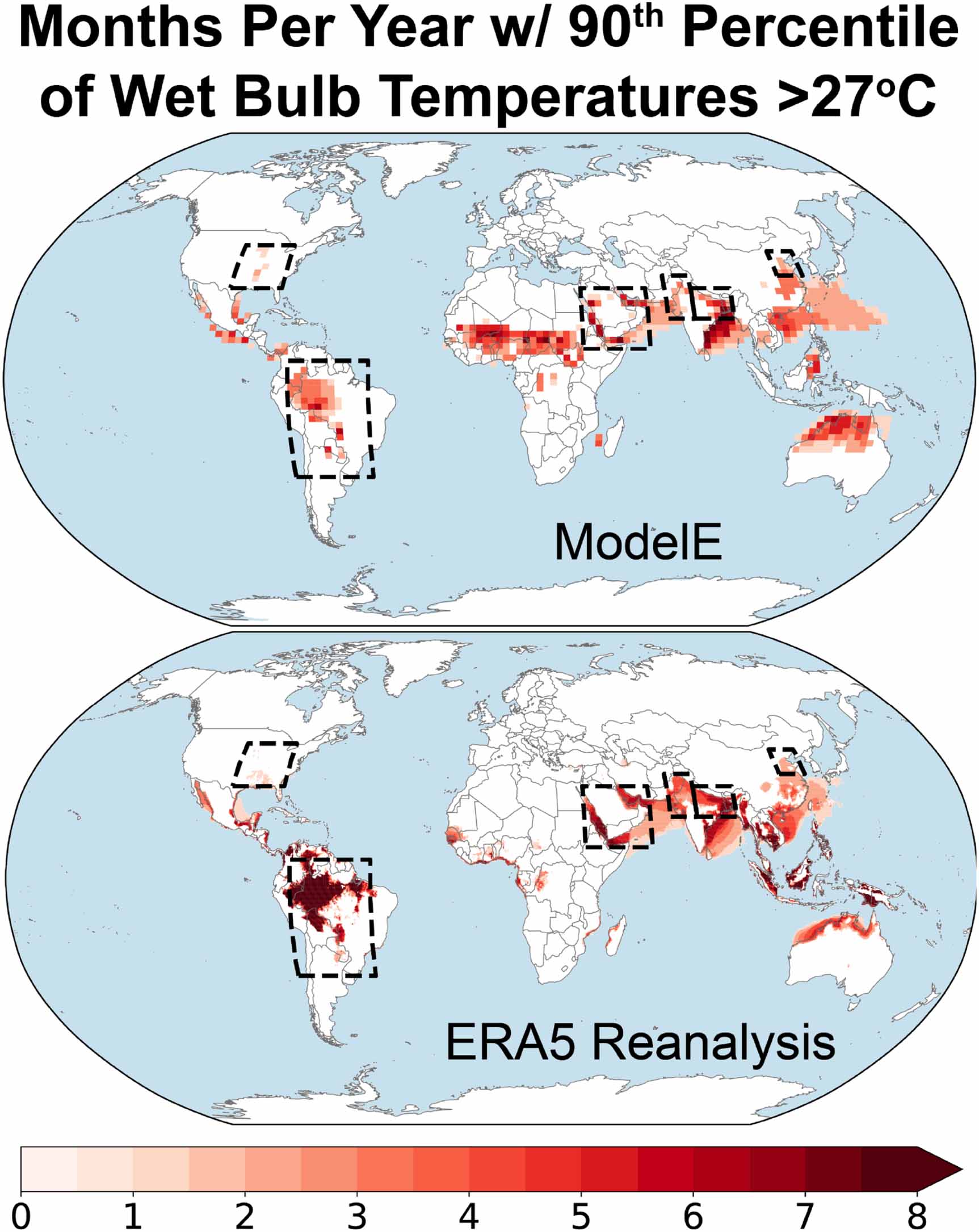
The distribution of hot locations in the ModelE Irrigation run, defined as the 90th percentile of maximum daily  reaching 27 °C at least one month per year (figure 1), included central North America around the Mississippi valley; the Amazon basin; the Sahel; parts of the Arabian peninsula; the northern and eastern Indian subcontinent; much of Southeast Asia and eastern China; and northern Australia. It also included extensive warm ocean regions, including the Red Sea, Persian Gulf, Bay of Bengal, both coasts of Central America, and the subtropical north western Pacific (figure 1). Global and regional averages here were taken over land areas, however. In general, this distribution agreed with that computed from ERA5 reanalysis fields (figure 1), and also with available weather station data [15, 47], although there were differences in detail, such as ERA5 showing more hot areas in Indonesia and fewer in Africa. Many of the differences are likely attributable to the higher resolution of ERA5 better representing topography and smaller-scale circulation patterns, as seen for example in its more complex pattern of hot locations over South and Southeast Asia. Also, the GISS ModelE run used idealized climatological forcings and sea surface temperatures, whereas interannual variability in ERA5 corresponded more closely with actual conditions.
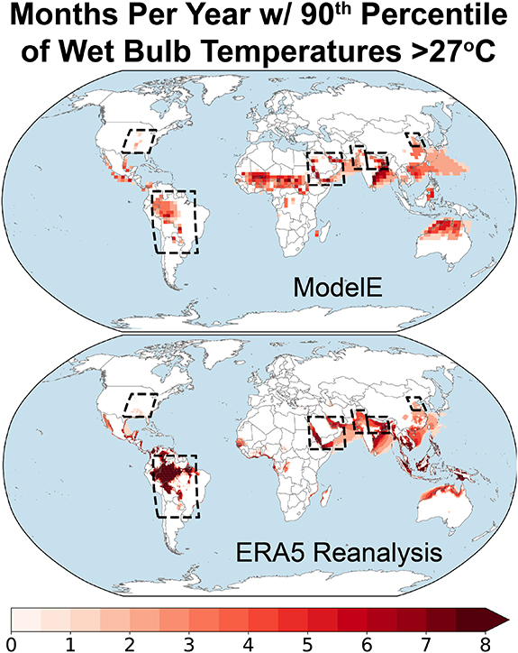
Figure 1. Months per year with the 90th percentile of daily maximum wet bulb temperature at least 27 °C, as derived from GISS ModelE (with irrigation) and the ERA5 reanalysis. Regions over which results are averaged are boxed.
Download figure:
Standard image High-resolution imageThe No-irrig run showed a very similar distribution of hot areas as the Irrigation run, though with some difference in detail, such as having fewer hot pixels in North America and Arabia (Supplementary figure S1 (stacks.iop.org/ERL/15/094010/mmedia)). To avoid any potential bias in averaging differences across the two ModelE runs, the hot locations and months analyzed below were defined as those that were hot in either of the two runs.
Many of the hot locations are densely populated agricultural areas. Particularly China and the Indian subcontinent have extensive application of irrigation during their hottest months (where hottest is defined based on 90th percentile of daily maximum wet bulb temperature; figure 2).
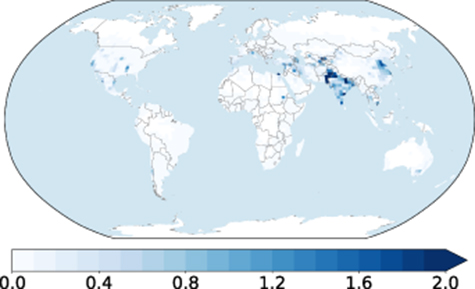
Figure 2. GISS ModelE irrigation rate for hottest month, mm d−1.
Download figure:
Standard image High-resolution imageFor hot months in land areas overall, irrigation results in a decrease of ∼ 0.1 °C in median daily maximum temperature (T50, figure 3) and an increase in humidity corresponding to a rise of ∼ 0.1 °C in median maximum dew point (T , figure 3). The cooling and higher humidity combine to yield a slight increase of ∼ 0.03°C in median wet-bulb temperature (T
 ), but no significant change in the 90th or 99th percentiles (figure 3). These changes are of the same sign in both irrigated and non-irrigated hot land areas, albeit the magnitudes of the cooling and humidifying are larger in the irrigated areas (figure 3).
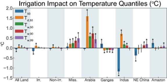
Figure 3. Impact of irrigation on temperature and humidity quantiles, averaged over hot land areas and months. T = surface air temperature; Td = dew point;  wet-bulb temperature. Subscript numbers refer to percentiles of daily maximums, computed for each grid cell and month and then averaged spatially. Starred Irrigation − No-irrig differences are significantly different from zero at the 0.05 level (two-tailed). The error bars show 95% confidence intervals.
Download figure:
Standard image High-resolution imageThe response to irrigation is not uniform across hot land regions (figure 3). Central North America's Mississippi valley, some of which is irrigated, shows no change in median temperature and an increase in dew point, and significant increases of 0.3–0.5 °C in 50th, 90th, and 99th percetile wet bulb temperatures. Arabia, mostly non-irrigated, shows no change in temperature and a large fractional increase in humidity, leading to an increase of 0.6 °C in median wet-bulb temperature and similar increases in extreme values. The adjacent, and heavily irrigated, Indus and Ganges valley areas show a contrast in responses. In the Ganges valley, temperature increases and dew point decreases, and wet-bulb temperatures decrease 0.1 °C. In the Indus valley, temperature decreases and humidity increases, leading to an increase of 0.1 °C in the median and 90th percentile wet bulb but no significant change in its 99th percentile. The irrigated North China Plain shows a decrease in median temperature and no change in median dew point; median wet-bulb temperature shows no significant change, but the 90th and 99th percentiles increase 0.1-0.2 °C. The non-irrigated Amazon basin shows a significant increase in temperature, presumably due to shifts in circulation patterns induced by irrigation, and no change in humidity, leading to a ∼ 0.1 °C increase in the 99th percentiles of wet bulb temperature.
Figure 4 shows the effect of irrigation on  across quantiles, averaged across all hot land areas and months. Quantiles of
  between about the 50th and 90th percentiles show significant warming due to irrigation. The lowest
  quantiles, corresponding to the coolest and least humid conditions in the hot areas and months, show cooling, primarily over non-irrigated areas such as the Amazon; this might be because a given fractional increase in relative humidity, such as might result from irrigation, elevates
  less when temperatures are cooler. The highest percentiles show no significant change, though for extreme quantiles the uncertainty due to finite sampling duration is greater (figure 4). The effects by quantile for individual regions vary, although the increases in
  due to irrigation in central North America, Arabia, and North China, as well as the decrease in the Ganges basin, are consistent across most quantiles (Supplementary figure S2).
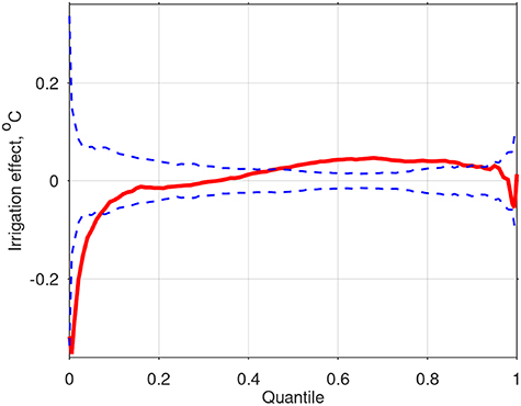
Figure 4. Mean effect of irrigation on quantiles of wet-bulb temperature over hot land areas. The dashed blue lines show the 95% confidence interval under the null hypothesis of zero effect.
Download figure:
Standard image High-resolution imageMapping the change in humid heat measures reveals more geographic detail. For example,  significantly increases with irrigation for most hot grid cells in central North America and Arabia (figure 5). In the Indian subcontinent, there is a decrease in
  over the Ganges valley and an increase in the upper Indus valley.
  tends to increase under irrigation in northeast China and decrease in southeast China. Some grid cells in the Sahel, northern Australia, and the Amazon basin, also show significant impacts of irrigation, despite little irrgation taking place nearby, and there are also significant impacts over some ocean areas, such as the East China Sea. These could be due either to direct impacts of irrigation (for example, if advected air from agricultural areas is moister due to irrigation, this could increase
  in a non-agricultural region) or to more indirect effects (such as changes in circulation pattern that more frequently advect air that is, for example, hot or moist to a given location). The typical magnitude of irrigation effects on
  is on the order of 0.4 °C (figure 5).
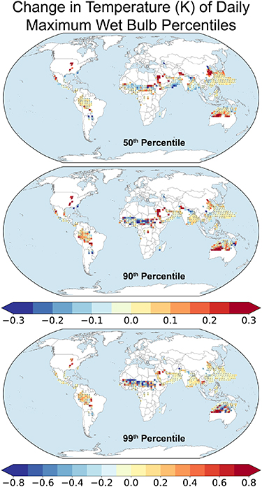
Figure 5. Mean effect of irrigation on the 50th, 90th, and 99th percentiles of daily-maximum wet-bulb temperature over hot months. Hatching shows where effects are not significant (that is, the effect size is consistent at the 95% confidence level with the null hypothesis of zero effect).
Download figure:
Standard image High-resolution imageChanges in the median wet-bulb temperature show mostly similar geographic patterns to changes in the 90th percentile, with somewhat smaller amplitude (figure 5). The more extreme 99th percentile of  shows larger amplitudes but fewer grid cells with significant differences (figure 5).
 is a function of temperature and humidity, which relate to the coupled water and energy balances. Precipitation changes between the No-irrig and Irrigation runs were not generally statistically significant, as differences due to irrigation were small compared to year-to-year variability (table 1). Under the Irrigation run, evapotranspiration and runoff, particularly underground runoff, increased over hot areas, particularly those with large amounts of irrigation (e.g. India and China; table 1). Surface sensible heat flux increased (became less negative) as a result of the surface cooling induced by the higher evaporation rate. Relative humidity also increased in irrigated areas. The Ganges valley region was an exception, with irrigation causing a weakening of summer monsoon flow such that surface solar flux increased, cloudiness decreased, and humidity did not significantly increase. Other hot regions showed mixed patterns that may reflect non-local influences of irrigation mediated by atmospheric circulation, with Arabia experiencing increased humidity and cloudiness, the Amazon experiencing reduced relative humidity, and the Mississippi basin showing little change (table 1). These regional climate changes due to irrigation could in some cases be associated with effects on
  (figure 3): for example, increased humidity in the Irrigation run over Arabia, the Indus, and China was associated with higher
  even though T decreased, while decreased cloudiness over the Ganges was associated with lower
  .
.
Table 1. Impact of irrigation on selected climate measures, averaged over hot land areas and months.
| All land | Irrigated | Non-irrigated | Mississippi | Arabia | Ganges | Indus | NE China | Amazon | |
|---|---|---|---|---|---|---|---|---|---|
| Precipitation (mm d−1) | −0.061 | −0.260 | −0.018 | −0.086 | 0.037 | −0.658 | −0.028 | −0.188 | −0.172 |
| Irrigation (mm d−1) | 0.166* | 0.932* | 0.004* | 0.558* | 0.024* | 0.810* | 2.532* | 1.023* | 0.000* |
| Evapotranspiration (mm d−1) | 0.076* | 0.330* | 0.022* | 0.140* | 0.017 | 0.182* | 1.374* | 0.299* | −0.036 |
| Surface runoff (mm d−1) | 0.001 | 0.068 | −0.013 | 0.023 | −0.000 | −0.063 | 0.424* | 0.025 | −0.017 |
| Underground runoff (mm d−1) | 0.041* | 0.177* | 0.012* | 0.099* | 0.000* | 0.140 | 0.228* | 0.204* | 0.000 |
| Surface net solar flux (W m−2) | 0.040 | 0.183 | 0.009 | 0.201 | −2.622* | 3.572* | −2.005 | −1.673 | 2.408* |
| Surface sensible heat flux (W m−2) | 1.459* | 6.782* | 0.336 | 2.562 | 0.507 | 1.547 | 29.800* | 7.216* | −2.268 |
| Relative humidity (%) | 0.410* | 1.801* | 0.117 | 0.773 | 1.476* | −0.071 | 8.595* | 1.552 | −1.267* |
| Cloud fraction (%) | 0.233 | −0.013 | 0.286 | −0.495 | 1.607* | −1.798* | 0.703 | 1.055 | −0.925 |
Starred Irrigation − No-irrig differences are significantly different from zero at the 0.05 level (two-tailed).
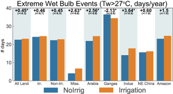
Dangerous conditions with T 27 °C slightly increased in frequency overall in hot areas due to irrigation, by a half day per year (going from 22.6 to 23.1 days) or 2% (figure 6). However, changes due to irrigation were pronounced over certain regions, with incidence almost doubling over hot locations in the Mississippi Valley region (from 4 to 7 days per year) and also increasing by 10-20% in Arabia and the Indus Basin, while decreasing some 6% over the Ganges Basin. Extremely dangerous conditions with T
 30 °C (not shown; 2.6 days per year overall in hot regions) showed no significant change in frequency due to irrigation overall, but increased significantly over Arabia (from 3.5 to 4.2 days per year), while decreasing significantly in the Indus basin (0.2 to 0.1 days per year).
Figure 6. Impact of irrigation on wet-bulb temperature exceedance frequencies (days per year), averaged over hot land areas.  = wet-bulb temperature. Starred Irrigation − No-irrig differences are significantly different from zero at the 0.05 level (two-tailed). The given uncertainties are 95% confidence intervals.
Download figure:
Standard image High-resolution image
4. Discussion and conclusions
The present work confirms the suggestions of some previous regional-scale research [19, 20, 48] that irrigation can increase wet-bulb temperature in hot months and days even while alleviating air temperature maxima. In fact, in the simulations presented here, irrigation on average significantly increased median daily maximum  over hot land regions and months, reflecting the combination of increasing humidity (Td) and decreasing temperature (T; table 3). While the mean increase in median
  due to irrigation was only ∼ 0.03°C, there was regional variation, with some hot regions, such as Arabia, experiencing much larger increases, while others, such as the Ganges basin, experienced decreases. The frequency of days with dangerously high
  similarly increased due to irrigation on average over hot regions, with some regions, such as the Mississippi Valley and northeast China, experiencing substantially greater likelihood of these high
  values.
The results here support a more nuanced approach to assessing the impact of irrigation and of land management in general on the potential for damaging heat. With few exceptions, previous studies of irrigation climate impacts have generally focused on its local and nonlocal cooling effects as alleviating heat waves, even while irrigation has been acknowledged to increase humidity [5, 49–53]. Also, many studies of the worsening potential for heat extremes use measures of heat based only on temperature, although projections of  increases under global warming are more robust than those for either temperature or humidity separately [10, 54].
  is a measure of humid heat that can be regarded as setting an ultimate limit on human adaptability [16, 55] and the impacts on it of irrigation as well as of greenhouse gas emissions and other climate forcings need to be understood in more detail. The impact of irrigation on other indices based on temperature and humidity that may better assess heat stress in particular contexts, such as wet bulb globe temperature (WBGT) [13, 56], should also be studied; WBGT is in fact often approximated as a weighted average of T and
  [11, 53].
One limitation of the studied model configuration is that SSTs were held fixed. Previous research has shown that compared with a fixed-SST configuration, feedbacks involving the oceans do not greatly modify simulated climate effects in irrigated areas, but do substantially modify and make more widespread climate effects of irrigation away from irrigated areas, in particular inducing wavelike spatial change patterns in high latitudes and in the Southern Hemisphere [3, 57]. Other limitations, which could also be addressed in future work, include using only one climate model, albeit one that has already been employed in several published analyses of irrigation climate impacts, and not considering the evolution with time of irrigated area extent as well as other climate forcings [2, 37]. For example, irrigation extent could decline in the future due to depletion of groundwater and surface water sources [58], or expand due to increased demand for food [59]. Additionally, although a global perspective such as the one taken here is of value, the higher spatial resolution of regional studies may well be able to more accurately represent heat extremes that are somewhat attenuated in a coarse-resolution global model, particularly in places like California where topographic variation is large [60, 61]. The differences found in some regions in the response to irrigation between different percentiles of  , for example in the North China Plain where irrigation did not significantly increase median
  but did worsen its extremes (figure 3), also deserves further investigation.
To summarize, in our climate model simulation, contemporary irrigation practices were found to overall reduce surface air temperature in hot regions and months but slightly increase the number of days with dangerously hot wet-bulb temperature, due to their effect on humidity. This underscores the need to consider humidity as well as temperature in assessing the impacts of irrigation and other climate forcings on the increasing likelihood of intense heat.
Acknowledgments
NYK gratefully acknowledge support from NOAA under grants NA16SEC4810008 and NA15OAR4310080 and by the United States Agency for International Development (USAID) under the U.S.-Pakistan Centers for Advanced Studies in Water. BIC and MJP were supported for this work by the NASA Modeling, Analysis, and Prediction program (NASA #80NSSC17K0265). Resources supporting this work were provided by the NASA High-End Computing (HEC) Program through the NASA Center for Climate Simulation (NCCS) at Goddard Space Flight Center. This is a Lamont Contribution. We also thank two anonymous reviewers for helpful comments that greatly improved our manuscript. All statements made are the views of the authors and not the opinions of the funding agency or the U.S. government.
Data availability statement
The data that support the findings of this study are available upon reasonable request from the authors.