

Abstract
Warming in the Arctic has resulted in a lengthening of the growing season and changes to the distribution and composition of tundra vegetation including increased biomass quantities in the Low Arctic. Biomass has commonly been estimated using broad-band greenness indices such as NDVI; however, vegetation changes in the Arctic are occurring at spatial scales within a few meters. The aim of this paper is to assess the ability of hyperspectral remote sensing data to estimate biomass quantities among different plant tissue type categories at the North Slope site of Ivotuk, Alaska. Hand-held hyperspectral data and harvested biomass measurements were collected during the 1999 growing season. A subset of the data was used as a training set, and was regressed against the hyperspectral bands using LASSO. LASSO is a modification of SPLS and is a variable selection technique that is useful in studies with high collinearity among predictor variables such as hyperspectral remote sensing. The resulting equations were then used to predict biomass quantities for the remaining Ivotuk data. The majority of significant biomass-spectra relationships (65%) were for shrubs categories during all times of the growing season and bands in the blue, green, and red edge wavelength regions of the spectrum. The ability to identify unique biomass-spectra relationships per community is decreased at the height of the growing season when shrubs obscure lower-lying vegetation such as mosses. The results of this study support previous research arguing that shrubs are dominant controls over spectral reflectance in Low Arctic communities and that this dominance results in an increased ability to estimate shrub component biomass over other plant functional types.
Export citation and abstract BibTeX RIS

Original content from this work may be used under the terms of the Creative Commons Attribution 3.0 licence. Any further distribution of this work must maintain attribution to the author(s) and the title of the work, journal citation and DOI.
1. Introduction
The Arctic has warmed at a greater rate than the rest of the globe through a process known as polar amplification (Serreze and Francis 2006, Walker et al 2012, Winton 2006). Global change in temperature from 1981–2012 is estimated to be 0.17 °C per decade (Hansen et al 2010), while warming in the Arctic (>66°N) has been approximately 0.60 ± 0.07 °C per decade (Comiso and Hall 2014) over the past century. Remotely sensed land surface temperature (LST) data from 1982–2008 indicate warming to be greater in the North American Arctic (+30%) than in the Eurasian Arctic (+16%) based on the Summer Warmth Index (SWI), which is the sum of average monthly surface temperatures above freezing (Bhatt et al 2010). Temperature increases have had probable effects on tundra ecosystems, such as a lengthening of the growing season (Huemmrich et al 2010, Zeng et al 2011), and associated increases in vegetation biomass, with Alaskan arctic tundra biomass increasing an average of 7.8% since the early 1980s (Epstein et al 2012).
Vascular and non-vascular (i.e. mosses and lichens) vegetation may respond differently to climate change (Huemmrich et al 2013). Mosses and lichens are often abundant in tundra ecosystems, though warming trends have led to atypical increases in vascular plant cover (Huemmrich et al 2013) and decreases in non-vascular cover (Walker et al 2006). This trend is not evident in all regions of the Arctic, and the High Arctic and alpine tundra have not experienced the same increases in vascular plant coverage (Cornelissen et al 2001). The observed increases in shrub abundance throughout the Low Arctic tundra (Myers-Smith et al 2011) may be due to their ability to outcompete other vegetation types, potentially through shading of non-vascular species (Chapin et al 1995, Cornelissen et al 2001, Sturm et al 2001).
Remote sensing has allowed scientists to monitor changes occurring in arctic vegetation at a variety of spatial and temporal scales (Stow et al 2004). Past studies have mapped changes in vegetation using aerial photography (Sturm et al 2005), coarse-scale satellite imagery such as that from the Advanced Very High Resolution Radiometer (AVHRR) (Walker 1999), and moderate-scale satellite imagery such as that from Landsat platforms (Muller et al 1999, Silapaswan et al 2001). Though vegetation change in the Arctic occurs on fine spatial scales with changes occurring at the species level, the use of high-resolution and hyperspectral imagery remains scarce (however, see Buchhorn et al 2013, Forbes et al 2010, Huemmrich et al 2013). Hyperspectral remote sensing allows for the use of information contained in more refined regions of the spectrum that might be obscured with broad-band data. This may be useful for identifying otherwise unobservable differences in vegetation structure and biochemical composition among plant tissue types in the Arctic.
Past studies have developed estimates of arctic tundra biomass using relationships with environmental factors (including other vegetation variables), such as SWI, gross primary productivity (GPP), and leaf area index (LAI) using simple regression (Epstein et al 2008, Riedel et al 2005a, 2005b, van der Wal and Stien 2014, Walker et al 2012) and multiple regression analyses (Ueyama et al 2013). Multiple studies have developed relationships between arctic tundra biomass and the remotely sensed broad-band Normalized Difference Vegetation Index (NDVI)—(e.g. Hope et al 1993, Raynolds et al 2012, Riedel et al 2005b, Stow et al 2004, Walker 2003). Shrubs contribute substantially to NDVI in the most southern areas of the arctic tundra, whereas bryophytes contribute relatively more to NDVI in the more northern subzones, where shrub cover is sparse (Raynolds et al 2012). Shrubs may become a more important component of tundra plant community biomass, as their cover and abundance increase with warmer temperatures (Riedel et al 2005b, Walker et al 1995).
Establishing relationships between plant tissue type biomass and hyperspectral information may be useful for tracking changes in arctic biomass occurring with increasing temperatures. Different regions of the visible and near infrared spectra can be used to identify functional and structural properties of vegetation communities and individual plant tissue types (Curran 1989, Ustin and Gamon 2010). Hyperspectral remote sensing (also known as imaging spectroscopy) has been useful in differentiating among vascular and non-vascular vegetation (Huemmrich et al 2013) and functionally distinct vegetation types in the Arctic (Buchhorn et al 2013). Moss and vascular plant spectra have similar reflectances in the green and near infrared (NIR) wavelength regions, whereas lichens have higher reflectance in the visible, and greater variability in species-specific reflectances (Huemmrich et al 2013). Dead biomass in the Arctic also influences the reflectivity spectra, particularly as shrubs begin to dominate these systems, and their leaf litter covers more low-lying plants (DeMarco et al 2014, Xu et al 2014).
Narrow-band NDVI combinations as well as other hyperspectral two-band vegetation indices (HTBVI) based on normalized difference between the bands have been used to describe biomass-spectra relationships, and show slightly better correlations with biomass than broad-band NDVI measurements (Buchhorn et al 2013). However, to date, hyperspectral data have not been evaluated for their utility in improving remotely sensed estimates of tundra biomass. The goal of this research was therefore to establish relationships between tundra biomass components and hyperspectral data from a Low Arctic site in Alaska using handheld hyperspectral remote sensing. Our specific objective is to develop relationships between a hierarchy of tundra vegetation biomass components (i.e. at landscape, plant community, plant functional type, and tissue type levels) and hyperspectral reflectance data. Analyses of these relationships across the various scales will inform the degree to which we can generalize relationships between tundra biomass and hyperspectral information.
2. Methods
2.1. Study area
Ivotuk, Alaska (68.49°N, 155.74°W) is located on the North Slope of the Brooks Mountain Range (Epstein et al 2004, Riedel et al 2005a, 2005b), and was one of seven sites established as part of the Arctic Transitions in the Land-Atmosphere System (ATLAS) project (McGuire 2003, Walker 2003, Walker et al 2003). Ivotuk is part of the Western Alaska Transect that starts in the north at Barrow and goes south through Atqasuk and Oumalik to Ivotuk (Epstein et al 2008, Jia et al 2002, McGuire 2003, Walker 2003).
Ivotuk is located in bioclimatic subzone E, which includes the Arctic Foothills and non-forested areas of the Seward Peninsula (Walker et al 2003). The Circumpolar Arctic Vegetation Map (CAVM) identifies five bioclimatic subzones (A-E) based on differences in climate, vegetation, topography, substrate biogeochemistry, and NDVI (CAVM 2003, Raynolds et al 2006, Walker et al 2005). Subzone E is the southernmost and warmest of the five tundra subzones. Ivotuk is largely a tussock tundra ecosystem also dominated by deciduous shrubs (Walker et al 2003). It is located at an elevation of approximately 550m (Epstein et al 2004). From 1991–2001 (a time period that encompasses the sampling that will be used for this research), the site received an annual average of 202 mm precipitation, had a July maximum temperature of approximately 12 °C, an annual temperature of −10.9 °C, and a 110-day growing season (Jia et al 2002, Riedel et al 2005a, 2005b).
The site of Ivotuk is comprised of the four plant communities: moist acidic tundra (MAT), moist nonacidic tundra (MNT), mossy tussock tundra (MT) and shrub tundra (ST). MAT and MNT are differentiated by soil acidity, with MAT occurring on soils with pH < 5.0–5.5, and MNT occurring on soils with pH ≥ 5.0–5.5 (Walker et al 2003, Walker et al 1994). MAT, also referred to as tussock-graminoid tundra, is dominated by dwarf erect shrub species such as Betula nana, and the tussock sedge Eriophorum vaginatum (Walker et al 1994). Betula nana is absent in MNT due to low soil acidity. Mosses, graminoids, non-tussock sedges, and prostrate dwarf shrubs such as Dryas integrifolia dominate in MNT communities (Jia et al 2004, Walker et al 1994). MT contributes greatly to biomass quantities in tundra systems, and is typified as an acidic tussock tundra with abundant Sphagnum mosses (Tenhunen et al 1992). ST is dominated by shrubs such as Salix alaxensis, Betula nana, and Alnus crispa (Muller et al 1999), and is interspersed with graminoids, forbs, lichens, and mosses.
2.2. Data collection and processing
One 100 m × 100 m grid was established in each of the four vegetation communities (Epstein et al 2008, Riedel et al 2005a, 2005b, Walker 2003, Walker et al 2003). Spectroscopy data were collected during the 1999 growing season at biweekly intervals from 5 June–26 August and grouped according to early and peak growing season (table 1). Spectral measurements were made using an Analytical Spectral Devices FieldSpec spectro-radiometer with a spectral resolution of 1.42 nm and a spectral range of 330.79–1061.78 nm (Riedel et al 2005a, 2005b). Spectral measurements were collected from ten random grid points established in each of the four vegetation grids. The same 10 points were used for spectral data collection for the duration of the growing season. Biomass data were collected biweekly from ten 20 × 50 cm plots adjacent to these spectral gridpoints (Epstein et al 2004, 2008, Riedel et al 2005a, 2005b, Walker et al 2003). Both biomass and spectral measurements were collected from an additional ten gridpoints for one collection week during peak growing season (Riedel et al 2005a, 2005b).
Table 1. Biomass sampling dates and observation count per vegetation community during the 1999 growing season, where n is the number of observations.
| Growing season | MAT | MNT | MT | ST |
|---|---|---|---|---|
| Early | 5 June–3 July (n = 22) | 8 June–10 July (n = 20) | 10 June–9 July (n = 20) | 6 June–11 July (n = 20) |
| Peak | 13 July–14 August (n = 28) | 25 July–22 August (n = 33) | 16 July–24 August (n = 24) | 26 July–23 August (n = 20) |
Vascular plants were clipped at the top of the moss surface, and mosses were clipped at the base of the green layer (Epstein et al 2004, Riedel et al 2005a, 2005b, Walker et al 2003). Biomass samples were sorted into seven functional categories including evergreen and deciduous shrubs, graminoids, horsetails, other forbs (hereafter simply 'forbs'), bryophytes, and lichens (Riedel et al 2005a, 2005b, Walker et al 2003). Samples were oven-dried at 55 °C for 48 h before being taken back to the University of Virginia for further processing (Epstein et al 2004). Graminoids were divided into live and dead materials (Riedel et al 2005a, 2005b). Evergreen and deciduous shrubs were divided into woody, foliar live, and foliar dead materials (Epstein et al 2004, Riedel et al 2005a, 2005b).
2.3. Species composition
Species data were collected using the Braun-Blanquet method (Westhoff and van der Meel 1973). Mosses were one of the most abundant plant functional types in all four communities (table 2). Hylocomium splendens (51%–75%) was the most common in MAT and ST, where the deciduous shrub Rubus chamaemorus also dominates species composition (51%–75%). The moss Tomentypnum nitens, the evergreen shrub Dryas integrifolia, and the graminoid Carex bigelowii all occurred with a frequency of (26%–50%) in MNT. Graminoids were the most abundant PFT in MT, with the largest contributor as the species Eriophorum vaginatum (51%–75%).
Table 2. Dominant plant species at Ivotuk, Alaska per plant vegetation community and plant functional type. Species are presented along with their Braun-Blanquet percentages. Most abundant species are shown in gray.
| Plant Functional Type | Vegetation Community | |||
|---|---|---|---|---|
| MAT | MNT | MT | ST | |
| Deciduous shrub | Betula nana ssp. exilis (26%–50%) | Salix reticulata (6%–25%) | Rubus chamaemorus (6%–25%) | Rubus chamaemorus (51%–75%) |
| Evergreen shrub | Rhododendron tomentosum subsp. decumbens (26%–50%) | Dryas integrifolia (26%–50%) | Rhododendron tomentosum subsp. decumbens (6%–25%) | Pyrola grandiflora (1%–5%) |
| Forb | Petasites frigidus (6%–25%) | Geum glaciale (6%–25%) | — | Petasites frigidus (26%–50%) |
| Graminoid | Eriophorum vaginatum (26%–50%) | Carex bigelowii (26%–50%) | Eriophorum vaginatum (51%–75%) | Eriophorum angustifolia (26%–50%) |
| Lichen | Baeomyces carneus, & Peltigera aphthosa (1%–5%) | Thamnolia vermicularis s. subuliformis (6%–25%) | Cladonia amaurocraea, C. arbuscula, C. stygia, Dactylina arctica, Flavocetraria cucullata, Peltigera rufescens, and Thamnolia vermicularis var. subuliformis (0.5%) | Peltigera leucophlebia (1%–5%) |
| Moss | Hylocomium splendens (51%–75%) | Tomentypnum nitens (26%–50%) | Sphagnum lenense (26%–50%) | Hylocomium splendens (51%–75%) |
2.4. Spectral processing
Original field spectroscopy data from Ivotuk were resampled to 5 nm wide hyperspectral narrowbands (HNBs) ranging from 400–1000 nm. Aggregating to 5 nm bands increases the signal-to-noise ratio (SNR), reduces wavelength redundancy issues, and potentially makes results more transferable to other sites and data that may have been collected with different instruments. As a quality assurance step, reflectance spectra from Ivotuk were examined visually for irregularities. Irregular spectra were removed before analysis in an effort to overcome the heterogeneous nature of vegetation at Ivotuk and develop a more diagnostic spectral signature.
2.5. Data analysis
Regularization methods such as the least absolute shrinkage and selection operator (LASSO) are valuable tools for addressing many of the analytical problems affecting hyperspectral remote sensing such as high collinearity. LASSO is a modified form of partial least squares regression that reduces model complexity using a regularization parameter and is unaffected by the order of variable entry into a model (Tibshirani 1996). The regularization parameter works by shrinking variable coefficients toward zero, and eliminating variables from the model when their coefficients reach zero. As such, LASSO is an effective variable selection and dimensionality reduction technique.
Data were first analyzed without separation by vegetation community, meaning that all biomass data from either early or peak season was used for analysis. This was then repeated with separation by MAT, MNT, MT, or ST community in order to establish relationships between biomass categories and spectral variables specific to a vegetation community. Sample size per vegetation community ranged from 20–22 during early growing season and from 20–33 during peak growing season (table 1). A simple random sample of one-half of the Ivotuk data was used to create the training set. The remaining one-half was used to create the test set. Plant tissue type biomass quantities were then regressed against spectra using LASSO regression from the 'glmnet' package in R (Friedman et al 2010).
3. Results
3.1. Total vegetation biomass
3.1.1. Biomass quantities
Total biomass across all four vegetation communities during early growing season was 768.9 g m−2. The greatest contributor to live biomass was moss (306.9 g m−2), followed by deciduous shrub (183.6 g m−2), evergreen shrub (61.9 g m−2), graminoid (37.1 g m−2), lichen (22.2 g m−2), and forb (8.7 g m−2) (figure 1).
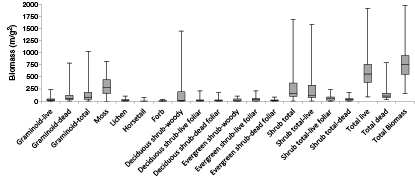
Figure 1 Boxplot of biomass quantities per plant tissue type during early growing season at Ivotuk, Alaska without separation by vegetation community.
Download figure:
Standard image High-resolution imageTotal biomass for all four vegetation communities during peak growing season was 851.2 g m−2. The greatest contributor to live biomass was moss (333.2 g m−2), followed by deciduous shrubs (155.0 g m−2), evergreen shrubs (89.0 g m−2), graminoid (58.8 g m−2), lichen (32.2 g m−2), and forb (10.8 g m−2) (figure 2).

Figure 2 Boxplot of biomass quantity per plant tissue type biomass component during peak growing season at Ivotuk, Alaska.
Download figure:
Standard image High-resolution image3.1.2. Optimal HNBs
The majority of hyperspectral narrow bands (HNBs) present in the biomass-spectra relationships for early growing season and without separation by community type were in the NIR wavelength region (725–1 000 nm) (figure 3). The next most common wavelength region was the blue (450–495 nm) followed by the NIR and green (495–570 nm), the red edge (680–725 nm) and yellow (570–590 nm). The least common wavelength region was red (620–680). No relationships used bands in the orange wavelength region (590–620 nm) of the spectrum. While the majority of HNBs used in significant biomass-spectra relationships were located in the NIR, those in the blue and green wavelength regions load more highly, and therefore more significantly affect the biomass-spectra relationships. Those in the yellow, orange, and red also load more highly than those in the NIR. The best relationships between plant tissue type and spectral reflectances were for deciduous shrub-live foliar and shrub total-live (adjusted r2 = 0.44) (figure 4, table 3).

Figure 3 Mean reflectance for all vegetation communities during early growing season along with the normalized coefficients for the optimal HNBs associated with the plant tissue type categories for total biomass.
Download figure:
Standard image High-resolution image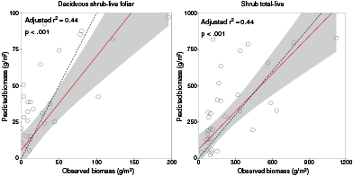
Figure 4 Best fit relationships between plant tissue type biomass components during early growing season without separation by vegetation community. The best-fit line is shown in red along with 95% confidence intervals shaded in gray. The dashed line is the 1:1 line.
Download figure:
Standard image High-resolution imageTable 3. Significant relationships during early growing season without separation by vegetation community.
| Plant Tissue Type | Predictor Bands | Adjusted r-square | p |
|---|---|---|---|
| Deciduous shrub-live foliar | 435, 440, 450, 520, 560, 565, 665, 860, 990, 995 | 0.44 | <.001 |
| Shrub total-live | 405, 450, 570, 665, 680, 710, 845, 850, 855, 990 | 0.44 | <.001 |
| Evergreen shrub-woody | 400, 440, 555, 560, 730, 765, 1000 | 0.43 | <.001 |
| Deciduous shrub-woody | 405, 450, 570, 660, 665, 855, 870, 990 | 0.40 | <.001 |
| Shrub total | 405, 445, 450, 570, 665, 680, 710, 845, 850, 855, 990 | 0.39 | <.001 |
| Deciduous shrub-dead foliar | 405, 475, 495, 540, 545, 570, 665, 685, 690, 695, 720, 850, 865, 880, 895, 965, 970, 990 | 0.33 | <.001 |
| Total-live | 445, 885, 890 | 0.31 | <.001 |
The majority of HNBs present in the biomass-spectra relationships for peak growing season and without separation by community type were in the near infrared wavelength and green wavelength regions (figure 5). The next most common was the red edge, followed by the NIR, blue and red, and finally orange wavelength region. In addition to being one of the dominant spectral regions, green wavelengths load more highly than most other segments. Blue also loads very highly, but is not one of the most common spectral regions in these relationships. Bands in the yellow, orange, red, and lower wavelengths of the NIR also load more highly than longer wavelengths. The best relationship during peak growing season without separation by vegetation community type was for shrub total-live (adjusted r2 = 0.65) (figure 6, table 4).

Figure 5 Mean reflectance for all vegetation communities during peak growing season along with the normalized coefficients for the optimal HNBs associated with the plant tissue type categories for total biomass.
Download figure:
Standard image High-resolution image
Figure 6 Best fit relationships between plant tissue type biomass components during peak growing season without separation by vegetation community. The best-fit line is shown in red along with 95% confidence intervals shaded in gray. The dashed line is the 1:1 line.
Download figure:
Standard image High-resolution imageTable 4. Significant relationships for plant tissue types during peak growing season without separation by vegetation community.
| Plant Tissue Type | Predictor Bands | Adjusted r-square | p |
|---|---|---|---|
| Shrub total-live | 400, 485, 490, 530, 590, 595, 690, 695, 715, 765, 985, 995, 1000 | 0.65 | <.001 |
| Deciduous shrub-woody | 400, 485, 490, 535, 600, 605, 695, 715, 825, 855, 860, 940 | 0.64 | <.001 |
| Shrub total | 400, 485, 490, 695, 715, 800, 805, 810, 825, 840, 845, 985 | 0.63 | <.001 |
| Deciduous shrub-live foliar | 490, 670, 940 | 0.39 | <.001 |
| Deciduous shrub-dead foliar | 485 | 0.32 | <.001 |
3.2. Biomass with separation by vegetation community
3.2.1. Biomass quantities
Shrub tundra had the greatest total biomass during early growing season (1063.3 g m−2), followed by MAT (683.5 g m−2), MT (679.6 g m−2), and MNT (657.9 g m−2) (figure 7). The plant tissue type that contributed the most biomass to MAT was graminoid-dead (173.6 g m−2). Moss was the greatest contributor in both MNT (462.5 g m−2) and MT (288.4 g m−2). Deciduous shrub-woody was the greatest contributor in ST (542.7 g m−2).
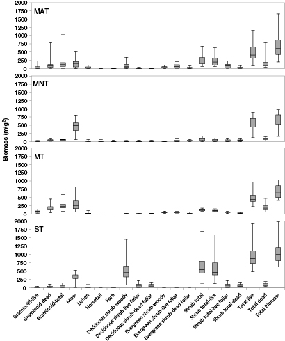
Figure 7 Boxplot of biomass quantity per plant tissue type biomass component during early growing season for vegetation communities of MAT (a), MNT (b), MT (c), ST (d) at Ivotuk, Alaska.
Download figure:
Standard image High-resolution imageST had the greatest total quantity of biomass during peak growing season (1129.1 g m−2), followed by MAT (842.2 g m−2), MT (815.2 g m−2), and MNT (724.8 g m−2) (figure 8). The largest plant tissue type biomass contributor was moss in all communities except ST at 201.5 g m−2 in MAT, 445.8 g m−2 in MNT, and 349.7 g m−2 in MT. Deciduous shrub-woody was the greatest contributor in ST at 498.3 g m−2.

Figure 8 Boxplot of biomass quantity per plant tissue type biomass component during peak growing season for the four vegetation communities of MAT (a), MNT (b), MT (c), ST (d) at Ivotuk, Alaska.
Download figure:
Standard image High-resolution image3.2.2. Optimal HNBs
The majority of HNBs for early growing season with separation by vegetation community type were located in the red edge wavelength region (figure 9). The next most common region of the spectrum was the green, followed by red, then blue, yellow, the NIR, and orange. Bands in the red edge wavelength region were dominant in MAT and MNT, while bands in the green wavelengths were dominant in ST. Bands in the red and red edge loaded highly in MAT, with bands in the blue and green loading highly for the relationship between MAT spectra and evergreen shrub-live foliar only. Bands in the red edge and the blue loaded highly for MNT, and bands in the green and red loaded highly in ST. The best relationship between biomass and spectral reflectances in MAT and ST was for evergreen shrub-live foliar (figure 10, table 5). MNT had two significant relationships with shrub total-live foliar and shrub total-live (adjusted r2 = 0.33).
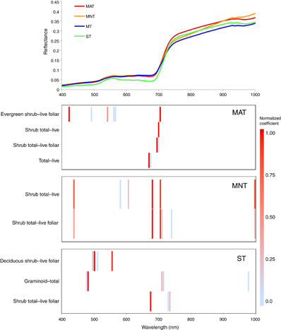
Figure 9 Mean reflectance for all vegetation communities during early growing season along with the normalized coefficients for the optimal HNBs associated with the plant tissue type categories for biomass per vegetation communities. There were no significant relationships for MT.
Download figure:
Standard image High-resolution image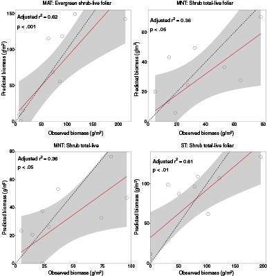
Figure 10 Best fit relationships between plant tissue type biomass components during early growing season for four vegetation communities at Ivotuk, Alaska. The best-fit line is shown in red along with 95% confidence intervals shaded in gray. The dashed line is the 1:1 line.
Download figure:
Standard image High-resolution imageTable 5. Significant relationships during early growing season for four vegetation communities at Ivotuk, Alaska.
| Community | Plant Tissue Type | Predictor Bands | Adjusted r-square | p |
|---|---|---|---|---|
| MAT | Evergreen shrub-live foliar | 420, 490, 540, 560, 565, 705 | 0.62 | <.001 |
| MAT | Shrub total-live foliar | 695, 700 | 0.56 | <.01 |
| MAT | Shrub total-live | 700 | 0.33 | <.05 |
| MAT | Total-live | 670, 675, | 0.33 | <.05 |
| MNT | Shrub total-live foliar | 435, 680, 705, 710, 740, 1000 | 0.36 | <.05 |
| MNT | Shrub total-live | 435, 580, 605, 680, 705, 1000 | 0.36 | <.05 |
| ST | Shrub total-live foliar | 675, 730, 735 | 0.61 | <.01 |
| ST | Graminoid-total | 475, 480, 710, 715, 980 | 0.59 | <.01 |
| ST | Deciduous shrub-live foliar | 495, 500, 510, 555 | 0.46 | <.05 |
The majority of HNBs for peak growing season with separation by vegetation community type were located in the red edge and blue wavelength regions (figure 11). The next most common region was the NIR, followed by yellow and green. No bands in the orange or red wavelength regions were used. Bands in the green and red edge were dominant in MNT, while bands in the red edge were dominant in MT. Bands in the blue and NIR were equally dominant in ST. Bands in the blue, red edge, and green load most highly in MNT. Bands in the blue load most highly in MT, and bands in the blue load more highly than those in the NIR in ST. MNT and ST both had significant relationships to shrub biomass tissue type, while MAT had no significant relationships, and MAT had relationships to total biomass and moss (figure 12, table 6).
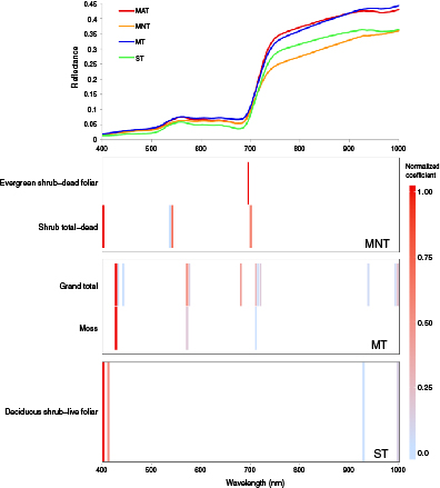
Figure 11 Mean reflectance for all vegetation communities during peak growing season along with the normalized coefficients for the optimal HNBs associated with the plant tissue type categories for biomass per vegetation communities.
Download figure:
Standard image High-resolution image
Figure 12 Best fit relationships between plant tissue type biomass components for vegetation communities during peak growing season. The best-fit line is shown in red along with 95% confidence intervals shaded in gray. The dashed line is the 1:1 line.
Download figure:
Standard image High-resolution image
Table 6. Significant relationships during peak growing season for four vegetation communities at Ivotuk, Alaska.
| Community | Plant Tissue Type | Predictor Bands | Adjusted r-square | p |
|---|---|---|---|---|
| MNT | Evergreen shrub-dead foliar | 695 | 0.48 | <.01 |
| MNT | Shrub total-dead | 400, 535, 540, 700 | 0.45 | <.01 |
| MT | Grand total | 425, 430, 440, 570, 575, 680, 710, 715, 720, 940, 995, 1000 | 0.42 | <.05 |
| MT | Moss | 425, 570, 710 | 0.36 | <.05 |
| ST | Deciduous shrub-live foliar | 400, 410, 930, 1000 | 0.44 | <.05 |
4. Discussion
This study uses LASSO regression to identify relationships between biomass categories and significant wavelengths in hyperspectral ground-based data in four vegetation communities at Ivotuk, Alaska. Biomass-spectra relationships were established both with and without separation by vegetation community type. Our results support the Riedel et al (2005b) findings that shrubs are dominant controls over spectral reflectances at Ivotuk, as 65% of significant biomass-spectra relationships were for shrub or shrub component parts. However, our findings suggest that areas of the spectra outside the typical range of broad-band NDVI (red: 620–680 nm; NIR: 725–1 000 nm) may be more useful for creating biomass-spectra relationships as bands in the blue (450–495 nm), green (495–570 nm), and red edge (680–725 nm) wavelength regions loaded very highly for the majority of biomass-spectra relationships. These findings support results by Bratsch et al (2016) indicating that bands outside typical NDVI ranges may be more useful for discriminating among vegetation community types than simply NDVI itself.
While mosses contributed the greatest quantities of biomass in vegetation communities at Ivotuk Alaska, the majority of significant relationships were for shrub vegetation at all times of the growing season, an aspect potentially due to shading by overlying shrub vegetation. Past research has highlighted the importance of live foliar shrub materials as dominant controls over spectral reflectance in MAT and ST, but has noted that graminoids and bryophytes tend to dominate in MNT and MT (Riedel et al 2005b). This research suggests that MAT, MNT, and MT all have spectral reflectances associated with shrub biomass while the peak MT spectral signature is closely associated with moss biomass, and is the only example of significant moss-spectra relationship in this study. Therefore, although mosses comprise large quantities of vegetation biomass, we may not be able to accurately estimate this biomass component due to shading from overlying vegetation.
There were twenty-six total significant relationships between plant tissue type biomass components and spectra at Ivotuk, Alaska (see tables 3–6). Seventeen significant relationships were for shrub or shrub component parts, six were for lower-lying plant tissue types such as dead biomass, graminoid, and moss; and three were for total categories. There were sixteen significant biomass-spectra relationships during early growing season but only ten during peak growing season. Stratification of vegetation by plant community type improved the relationships between spectral reflectance values and biomass only during the early growing season. During the peak of the growing season, these relationships worked well across all four vegetation types analyzed. If the vegetation type-specific relationships were to be used, these communities can be discriminated among each other, also using hyperspectral data (Bratsch et al 2016).
Differences in composition of vascular and non-vascular vegetation determine many of the spectral differences among vegetation communities in the Alaskan Arctic (Huemmrich et al 2013). Biomass-spectra relationships per individual community are stronger during early growing season, which may be attributable to less shrub coverage, and more contribution from non-vascular plant species to spectral signatures. These results suggest that differences in biomass-spectra relationships are more apparent during early growing season, and decrease during peak growing season, resulting in a decreased ability to develop significant relationships between biomass and spectra during peak growing season at the individual community level. The problem with establishing biomass-spectra relationships for individual communities during peak growing season may be attributable to increased shrub cover during peak growing season, shading of non-vascular vegetation, similarities in species composition, and shrubs obscuring spectral information from underlying vegetation. These results suggest that community separation may be a better method for establishing biomass-hyperspectral relationships during early growing season, while analyses without community separation may be a better method during peak growing season.
Overall, hyperspectral bands associated with pigments (400–700 nm) loaded highest when establishing biomass-spectra relationships without separation by vegetation community type during both early and peak growing season. Bands in the NIR that are associated with plant structure were only significant for four relationships during early growing season with separation by vegetation community type. These relationships were for live and live foliar shrub components. Unlike (Bratsch et al 2016) where vegetation structure becomes more important for community discrimination during peak growing season and reliance on NIR bands increases, in this study, the high loading of wavelengths in the green and blue remains consistent during all times of the growing season. This indicates a strong reliance on hyperspectral wavelengths associated with chlorophyll absorption during all parts of the growing season. Bands associated with chlorophyll in general, some of these outside the typical range of broad-band NDVI, are the most significant for determining biomass quantities at Ivotuk, Alaska.
5. Conclusion
Arctic vegetation communities vary in plant species and plant functional type composition and biomass quantities. Along with physiological features in plant species, these differences result in spectral variations that are identifiable through hyperspectral remote sensing, and allow for the creation of biomass-spectra relationships. This study presents an example of the use of hyperspectral information for establishing these biomass-spectra relationships. This allows us to create remote ways of tracking increases in biomass quantities with climate change without incurring the large monetary and time cost traditionally associated with arctic research. The above research presents a method for developing biomass-spectral relationships using handheld hyperspectral data that can then be used to identify bands on upcoming satellite missions such as the NASA Hyperspectral Infrared Imager (HyspIRI) and the German Environmental Mapping and Analysis Program (EnMAP) that would be useful for tracking changes in vegetation biomass. Establishing these relationships at the ground level allows for the potential use of these methods to monitor changes to biomass occurring with increasing temperatures in the Arctic at much larger spatial and longer temporal extents.