


Abstract
There is an active debate regarding the influence that climate has on the risk of armed conflict, which stems from challenges in assembling unbiased datasets, competing hypotheses on the mechanisms of climate influence, and the difficulty of disentangling direct and indirect climate effects. We use gridded historical non-state conflict records, satellite data, and land surface models in a structural equation modeling approach to uncover the direct and indirect effects of climate on violent conflicts in Africa and the Middle East (ME). We show that climate–conflict linkages in these regions are more complex than previously suggested, with multiple mechanisms at work. Warm temperatures and low rainfall direct effects on conflict risk were stronger than indirect effects through food and water supplies. Warming increases the risk of violence in Africa but unexpectedly decreases this risk in the ME. Furthermore, at the country level, warming decreases the risk of violence in most West African countries. Overall, we find a non-linear response of conflict to warming across countries that depends on the local temperature conditions. We further show that magnitude and sign of the effects largely depend on the scale of analysis and geographical context. These results imply that extreme caution should be exerted when attempting to explain or project local climate–conflict relationships based on a single, generalized theory.
Export citation and abstract BibTeX RIS

Original content from this work may be used under the terms of the Creative Commons Attribution 4.0 license. Any further distribution of this work must maintain attribution to the author(s) and the title of the work, journal citation and DOI.
1. Introduction
Although there is a suggested linkage between violent conflict and climate, the underlying mechanisms of the link are still under debate [1, 2]. One commonly suggested mechanism is of a climate–conflict link through economic disruption [3, 4]. Though plausible, there is currently no robust evidence for such a direct climate–economy–conflict nexus [5]. Instead, many studies suggest that climate-driven depressions may lead to conflict through a combination of socioeconomic and political failures, particularly in agricultural-dependent regions where people depend directly on such resources [4]. That is, climate influences economy, which influences social and political systems relevant to conflict.
It is also possible that the climate–conflict connection is less direct, operating through the influence that climate-induced changes in economy, food security, or group interactions cascade to influence the probability of inter-group violent conflicts. This indirect influence is relevant to theories like the 'engagement' hypothesis, which claims that when climate crisis reduces economic productivity people become more likely to engage in conflicts than in economic activities [6, 7], or the 'inequality' hypothesis, which argues that conflict may upsurge when climate crisis increases economic inequality because of increasing efforts to redistribute assets [8], and the 'state weakness' hypothesis that suggests a weakening of governmental institutions and their ability to suppress violence due to decline in economic productivity following climate crisis [9]. All these, suggest that climate has an indirect rather than a direct effect on violent conflicts [10].
While these hypotheses were first studied in the context of civil wars and other state-engaged conflicts, research in the past decade on communal, non-state violence has also emphasized the mediated pathways through which climate can influence conflict. This includes the potential for harmful climate anomalies like drought to drive conflicts in times of scarcity due to resource competition, lowered opportunity cost, or other mechanisms [11, 12]. But it also includes the potential for beneficial climate anomalies to increase conflict due to rent seeking or available resources to support violent activities during times of abundance [13, 14]. Studies have also found that climate variability in either direction can lead to increased conflict, due to the presence of multiple mechanisms driving conflict or to the presence of qualitatively different categories of conflict [15, 16].
The direct influence of climate on individual tendency toward violence may also play a role. Warming, for example, has been shown to enhance violence through a direct psychological mechanism [the General Aggression Model—GAM] by making people uncomfortable and irritated [17]. Alternatively, warming may enhance violence in cooler environments because warm, more favorable weather conditions lead to increased activity and interaction between people [Routine Activity Theory—RAT], which may lead to more opportunities for conflict [18].
To assess climate impacts on violence and uncover whether the underlying mechanisms are direct, indirect, or a combination of both, 'non-climatic' effects must be isolated. Some studies do this by pooling data across locations and applying statistical models that control for non-climatic factors explicitly. The climate influence is then examined through its partial effect on violence [19, 20]. Other researchers argue that controlling for non-climatic factors explicitly can absorb most of the climatic impact and, therefore, may result in an underestimation of the climate effect [21]. For this reason, it is argued, pooling analysis across sites is misleading, and climate effects should be studied by comparing each place with itself in time rather than with other places. Studies using this site self-comparison approach have reached more conclusive results regarding climate impacts on violence than cross-sectional studies using explicit controls [21, 22]. The problem with this self-comparison approach, however, is that it cannot identify underlying 'universal' mechanisms because the analysis is conducted location-by-location rather than across locations [23].
To some extent, the contrasting results published in the literature are a reflection of that disagreement [24], with this inconsistency leading to criticism of climate–conflict research. Some researchers have claimed that the link between climate and conflict is unsupported by the evidence [25]. Furthermore, researchers have been accused of bias in their approach to the problem [26, 27]. Yet, most experts do believe that climate has a significant effect on human conflicts [28], though the generality of the links and the underlying mechanisms are yet to be established.
Here we use a powerful assemblage of disaggregated data (table S1 (available online at stacks.iop.org/ERL/15/104017/mmedia)), which includes the Uppsala Conflict Data Program (UCDP) conflict dataset [29] as well as climatic [temperature and rainfall anomalies] and non-climatic [anomalies in water availability, infant mortality rates, agricultural yield, and economic welfare] datasets derived from satellites and land surface models to test generalizability of climate–conflict relationships from national to continental scale. To leverage the strengths of the two approaches—the site self-comparison and the use of explicit controls in a cross-sectional analysis—and explore general mechanisms, we make use of structural equation modeling [SEM] [30] in which non-climatic factors are explicitly controlled while direct and indirect effects of climate—through the non-climatic factors—are quantified in order to uncover the underlying mechanisms.
We choose to focus on non-state conflicts rather than civil wars because small-scale conflicts are likely to be more sensitive to environmental and climatic changes [19, 28]. Also, we focus on Africa and the Middle East [ME] because these two regions experienced a large number of armed conflicts in the last three decades. Finally, we hypothesize that comparing these two ethnically and culturally distinct, but yet geographically close regions may reveal contrasting mechanisms.
2. Data and methods
2.1. Armed conflict dataset
2.1.1. The UCDP geolocated violent conflict dataset
We used the most updated Georeferenced Event Dataset [GED] Global version 18.1 (2017) of the UCDP [29] for location-specific information on armed conflicts in Africa and the ME. The GED.v18.1 is UCDP's most disaggregated data set, covering individual events of organized violence as phenomena of lethal violence occurring at a given time and place. Events are sufficiently fine-grained to be geo-coded down to the level of individual villages, with temporal durations disaggregated to single, individual days [31]. Conflicts used here are 'non-state' conflicts, defined by UCDP as 'the use of armed force between two organized armed groups, neither of which is the government of a state, which results in at least 25 battle-related deaths in a year' [31]. Information on specific conflict is freely available at [www.ucdp.uu.se], and questions regarding the definitions used by UCDP as well as the content of the dataset can be directed to that site. In the GED dataset, each conflict has a unique identifier [conflict ID], while the start date is recorded as precisely as possible with the level of precision for day, month and year indicated alongside ['Startprec' variable in GED.v18.1].
For our analysis we used conflicts indicated with a 'Startprec' level of at least five meaning that 'Day and month are assigned, year is precisely coded; day and month are set as precisely as possible'. A violent event was defined as a coded event, which is unique in terms of starting and ends dates, and is not a continuation or part of a previous event. All events were first binned at a spatial resolution of 0.5 × 0.5
× 0.5 for African and ME regions by summing the total number of events per grid per year. Events were assigned to a specific year by indicated starting date. A layer of violent events by 0.5
 per year was produced alongside another layer with the sum of events for the entire period of 1990–2017 . Because we look for effects on the risk of violent conflict outbreak, each layer was converted into a binary layer in which each grid was assign a value of 1 for grids that experienced violence during this year, or 0 for grids that did not experience violence. Although we had information on violence for 1990–2017, we used only layers for years 1992–2012 in the SEM analysis because this was the period in which we had a complete data set of climate and non-climate variables (see below). We included Syria in our analysis, but excluded the years after 2010 because of the poor information on violent events during the period of the Syrian civil war [31, 32].
2.2. Climate data
We used temperature and rainfall data sets, described below, to seek direct and indirect effects of temperature and rainfall anomalies on non-state conflicts. Direct effects of climate could be only at the time of occurrence, so relationships were analyzed for the same year (present-year violence). However, indirect effects—through food, water, and economic welfare—may occur at a certain time-lag. Because linking climate anomalies indirectly to conflicts at too long time-lag periods may be problematic (because of the uncertainty that such climatic changes are really related to conflicts many years after), we looked only for links with a one-year time lag (next-year violence).
2.2.1. Temperature anomaly
We used monthly maximum temperatures from the newly derived Climate Hazards center InfraRed Temperature with Stations [CHIRTS] dataset [33]. CHIRTS provides monthly 2 m maximum air temperatures at a high spatial resolution of 0.05° and a quasi-global coverage [60°S–70°N] from 1983 to 2016. Temperature estimates are derived using a combination of thermal imagery from a constellation of geostationary satellites, a high-resolution climatology from the Climate Hazards Center's Tmax climatology, and in situ monthly 2 m Tmax air temperature observations obtained from the Berkeley Earth and Global Telecommunication System [GTS]. We used the temperature estimates from CHIRTS because these were shown to be suitable for monitoring temperature anomalies and extremes in data-sparse regions like Africa and the ME [33]. The high spatial resolution temperature estimates were averaged over 0.5° × 0.5° for the period of the analysis [1992–2012], and the yearly anomaly was calculated per grid as z-score [the long-term mean annual temperature was subtracted from the specific year mean temperature and divided by the standard deviation].
2.2.2. Rainfall anomaly
For rainfall anomaly, we used the Climate Hazards center Infrared Precipitation with Stations [CHIRPS] dataset, available at a high spatial resolution of 0.05° [34]. This product is a quasi-global precipitation product with daily to seasonal time scales and a 1981 to near real-time period of record. CHIRPS uses three main types of information: (1) global 0.05° rainfall climatologies, (2) time-varying grids of satellite-based rainfall estimates, and (3) in situ rainfall observations. CHIRPS is built on 'smart' interpolation techniques and high resolution, long period of record estimates based on infrared cold cloud duration [CCD] observations as well as on satellite information, used to represent ungauged locations. CHIRPS is quite reliable in regions like Africa and the ME where most rainfall products fail to accurately represent the high temporal and spatial variability in rainfall [35] due to the sparse gauge network in this region [36].
We used CHIRPS monthly rainfall sums [from January to December] to assess the annual rainfall anomaly for 1992–2012, calculated as z-scores [the long-term mean annual rainfall subtracted from specific year rainfall sum, divided by the standard deviation]. Each year a z-score map was produced while pixels were aggregated to the spatial resolution of the analysis [0.5° × 0.5°]. Annual rainfall is not a comprehensive proxy for conflict-relevant rainfall variability, but it offers a practical, objective measure that can be applied consistently across our diverse study domain.
2.3. Non-climate data
2.3.1. Infant mortality rate
As a proxy of socioeconomic development, we used information on infant mortality rate [IMR] from the Global Subnational Infant Mortality Rates, Version 1 [GSIMR.v1] [37]. The GSIMR.v1 dataset is produced by the Columbia University Center for International Earth Science Information Network [CIESIN] at a high spatial resolution of 5 km and is freely available for download as a raster data layer from [http://www.ciesin.columbia.edu/povmap]. The GSIMR.v1 consists of IMR estimates for the year 2000, which was collected from vital registration data, surveys and models or estimated using reported live births and infant deaths data. Though our analysis spans the period of 1992–2012, we assume that the 2000 GSIMR.v1 is, in average, representative of the entire period following previous studies [38]. The IMR is calculated as the number of deaths of infants of less than one year old divided by the number of live births and multiplied by 1000. We preferred using the IMR as a proxy of poverty and socioeconomic status instead of using other variables because measures like gross domestic product [GDP] or population living on less than one U.S. dollar per day, are difficult to obtain at sub-national levels, particularly for the regions of this study. Moreover, using IMR has several advantages over other socioeconomic metrics. For example, IMR is a highly standardized measure compared to other measures, which means that it can be used to compare between countries with different economic systems better than GDP, for example [38]. Also, IMR is less likely to be influenced by skewed wealth distribution. And, information on IMR is available for 90% or more of the population in medium- and low-income countries. The original 5 km IMR data layer was binned at the spatial resolution of 0.5° × 0.5°, which is the resolution of the analysis and used as a static map layer.
2.3.2. Distance to border
Distance from/to political borders was assessed using a geographical information system and a shapefile layer of the political borders of African and the ME countries. The minimal distance from each grid cell to the nearest border was recorded and used in the SEM analysis. Because this information is static [i.e. it does not change during the period of analysis] the same value was used in all years.
2.3.3. Agricultural dependence
To assess agricultural dependence as share of cropland area in a 0.5° grid cell, we used the Climate Change Initiative [CCI] of the European Space Agency [ESA] Land Cover product. The ESA CCI product is an annual global land cover time series from 1992 to 2015 [now available also for 2016 to 2018], available at an unprecedent high spatial resolution of 300 m (https://www.esa-landcover-cci.org/?q=node/175). This unique dataset was produced by reprocessing and interpretation of daily surface reflectance of five different satellite missions. It uses the full archive of the MEdium-spectral Resolution Imaging Spectrometer (MERIS) [2003–2012], with 15 spectral bands and 300 m spatial resolution and the 1 km time series from AVHRR [1992–1999], SPOT-VGT [1999–2013] and PROBA-V [2014 and 2015]. The baseline was established through MERIS data and use of machine learning and unsupervised algorithms [39].
The advantage of this product over other products that are derived from several observation systems is that it maintains a good consistency over time. This is done by confirming changes observed in earlier and later MERIS era satellites via back- and forward-checking through the 10 year MERIS base-line Land Cover (LC) maps. The ESA CCI LC product was evaluated with a global independent validation dataset according to international standards, testing the accuracy of both LC classes and LC change in time [39]. It was also found accurate through a comparison using country-level information provided by the Food and Agriculture Organization of the United Nations [FAO-STAT] in several countries [40].
We used the 1992–2012 ESA CCI LC maps to classify pixels into agricultural versus non-agricultural classes. More specifically, LC classes #10, 20, 30, and 40, which include also mosaics of croplands and natural vegetation, were designated as agricultural pixels while others were assigned as non-agricultural pixels. We then aggregated the 300 m pixels into the coarser resolution of 0.5° [resolution of analysis] and calculated the total share of agricultural area in each 0.5° grid cell [as the percentage of total area]. These estimates were used to examine influence of agricultural dependence [larger crop share of area equals higher agricultural dependency [38]] on violence risk as well as to derive yearly change in agricultural yield production [see next sub-section].
2.3.4. Yield production
To quantify changes in agricultural yield production, we used NASA's VIPPHEN EVI2 satellite product [41]. The VIPPHEN EVI2 data product is provided globally at 0.05° [5600 m] spatial resolution and contains 26 Science Datasets [SDS], including phenological metrics such as the start, peak, and end of season as well as the maximum, average, and background calculated EVI2 (https://lpdaac.usgs.gov/products/vipphen_evi2v004/). It is currently the longest and most consistent satellite-based global vegetation phenology product available. VIPPHEN SDS are based on the daily VIP product series and are calculated using a 3 year moving window average to eliminate noise.
The modified 2-band enhanced vegetation index [EVI2] is highly correlated with the commonly-used EVI [42], which was found to be useful for tracking changes related to vegetation dynamics [43] as well as gross primary productivity [44]. EVI2 differs from the traditional EVI by its use of two bands, the red and near infrared, instead of the use of three bands, which also includes the blue band in the index calculation. The integral over the growing season of EVI2 [EVIGSI; figure S1] was used here as a proxy of agricultural yield production. Growing season integrals of vegetation indices are usually well correlated with biomass of green tissues, particularly in annual vegetation systems [45–47], and as such may serve as a good proxy of crop yield production [48]. EVIGSI was derived per year for agricultural pixels with > 50% of agricultural area cover [estimated from the ESA CCI LC 300 m product]. Pixels with < 50% of agricultural area cover were discarded from the analysis in order to remove influences of non-agricultural vegetation systems on EVIGSI.
Because agricultural fields differ in crop type and different crop types may have similar EVIGSI values, we used the relative anomaly of EVIGSI as a proxy of relative anomaly in local yield production instead of the absolute EVIGSI value. In order to assess the validity of this approach, we compared yearly anomalies of national yield production, derived from the food and agriculture data provided by the Food and Agriculture Organization of the United Nations [FAO-STAT [49]], with country-level EVIGSI anomalies (z-scores) for the period of analysis [1990–2012; see supplementary material and figures S2 to S5]. Yield is provided in FAO-STAT as hectograms per hectare [hg/ha] for cereals, citrus fruit, coarse grain, fibre crops, oil-crops, pulses, roots and tubers, treenuts, vegetables and fruits (www.fao.org/faostat/en/#data/QC). The total annual yield and the long-term mean annual yield [1990–2012] from FAO-STAT were calculated to derive the relative anomaly in percentages of the long-term average yield [%]. The same procedure was applied for the calculation of the EVIGSI annual anomaly [as percentages of the mean EVIGSI].
2.3.5. Satellite night-time lights as a proxy of economic welfare
We used night-time lights intensity from the Defense Meteorological Satellite Program [DMSP [50]] to estimate grid-based economic welfare status and dynamics in Africa and the ME. This night-time light product dates back to 1992 and is considered to be well correlated with GDP, built-up area, energy consumption, poverty, and other socioeconomic welfare variables [51–54]. We used the DMSP yearly average stable night-time lights intensity product at a spatial resolution of 30 arcsec [1 km] for 1992–2012 to calculate the percentage area of light per pixel [LitArea]. Method was followed by that described in [55]. In short, light intensity in DSMP is given as a digital number [DN] from 0 to 100 for each pixel. A DN threshold value is then used to assign each pixel with a binary 1/0 for presence/absence of light. The threshold of DN > 31 was used following [55]. The total LitArea per 0.5° grid—i.e. the sum of the squared kilometers of light in a 0.5° grid cell—was derived by aggregating pixels with values to the spatial resolution of the analysis. The total number of square kilometers was then converted into square meters and divided by the population density in the same grid cell to derive the relative LitArea [R-LitArea].
We divided the LitArea by the population density because places with denser populations are expected to have higher LitArea, which will not necessarily indicate a higher economic welfare status but may just reflect a larger build-up area. By dividing the LitArea by the population density, we thus normalize for such an effect, remaining with a relative measure of economic welfare. We used the WorldPop dataset [www.worldpop.org.uk] for grid-based information on population density. This dataset uses an ensemble learning method for classification, combining 30 m Landsat Enhanced Thematic Mapper (ETM) satellite imagery for high-resolution mapping of settlements and gazetteer population numbers to produce gridded population density maps at high spatial resolutions [56]. Yearly population maps for Africa and the ME are available from 2000 to date [downloaded from: https://www.worldpop.org/project/categories?id=3] at the same resolution of the DMSP dataset [1 km × 1 km]. We used simple linear interpolation to derive population density for 1992–1999, and aggregated the original resolution to the coarse spatial resolution of the analysis [0.5° × 0.5°]. R-LitArea was derived per 0.5° grid cell as the ratio between LitArea and population density. Finally, R-LitArea z-score was calculated to get yearly economic welfare anomaly.
2.3.6. Grid-based water resources information from land surface models
Gridded estimates of soil moisture and hydrological fluxes, along with river network estimates of streamflow, were generated using the NASA Land Information System [LIS] [57] software frameworks. In this implementation, LIS was implemented using the Noah-MultiParameterization [Noah-MP] [58] Land Surface Model and the Hydrological Modeling and Analysis Platform [HyMAP] [59] river routers. All simulations were performed using meteorological forcing data drawn from the NASA Modern Era Reanalysis for Research and Applications, v2 [MERRA-2] [60], with the exception of precipitation, which came from the Climate Hazards InfraRed Precipitation with Stations, v2 [CHIRPSv2] [34] dataset. Simulations were performed at 0.1 horizontal resolution with a timestep of 30 min. A 30 year spin-up was performed to equilibrate model soil moisture states, and the simulation was then run from 1990–2018. In this application, Noah-MP was used with four soil moisture layers [thicknesses of 0.1, 0.3, 0.6 and 1.0 m, descending from the surface] and a simple unconfined aquifer. Soil moisture and surface runoff were aggregated to the spatial resolution of the analysis and the z-score of each 0.5° grid cell was calculated to derive the inter-annual anomaly.
3. Assessing direct and indirect causal effects
The SEM approach was used because it allows one to evaluate direct and indirect effects of climate and non-climate factors on violence risk, as well as to quantify relationships among factors. In that sense, SEM has an advantage over univariate regression approaches, such as general additive models (GAM) and general linear models (GLM), because it can be used to evaluate direct effects while controlling for joint effects. For example, it provides a way to evaluate the direct effect of yield on conflict risk while controlling for the joint effects of climate variables on yield and conflict. The ability of SEM to quantify direct and indirect relationships makes it particularly suited for confirming causal relationships based on a priori hypotheses.
Our SEM was developed based on a conceptual model designed to test a priori hypothesis that relates climate to food and water security, economic welfare and—directly and indirectly—to conflict risk [6–9]. It was then applied on a 0.5° grid basis in a time-for-space model design for 1992–2012 (see supplementary material). The SEM model was applied for Africa, the ME, and both regions together, as well as for each country separately. To enable comparison between datasets with different normal distributions, we used the relative anomaly—quantified as a standard score [z-score]—instead of the absolute values of the climate and non-climate factors. The control variables [IMR, agricultural dependence and distance to border], on the other hand, were maintained with their absolute values in order to quantify the absolute influence of these factors on the climate-conflict relationships. The conflict data were converted to a binary dataset, with 0 for non-conflict and 1 for conflict years/grids. The results of the SEM are presented as standardized effects indicating the magnitude and sign of effect.
4. Results and discussion
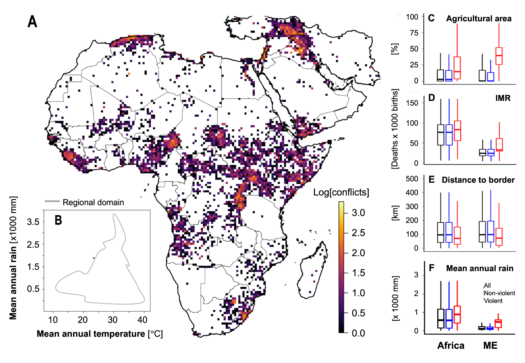
Non-state armed conflicts in the last three decades were not restricted to certain climatic conditions in Africa and the ME but rather occupied the entire climatic domain (figure 1(A) to(B)). Consistent with previous studies, violent conflicts are mostly found in agriculture-dependent areas [38], low socioeconomic areas [61], and close to political borders [19] in both regions (figures 1(C) to (E)).
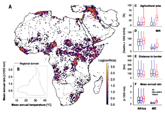
Figure 1. Armed conflicts in Africa and the Middle East, and associated factors. (A) Log number of armed conflicts by 0.5° grids for 1990–2017. (B) Mean annual rainfall and temperature binned by log number of conflicts. Gray line in (B) marks the region's climatic domain (95th quantile of all grids). Boxplots show median, 1st and 3rd quantiles of (C) relative agricultural area, (D) infant mortality rate (IMR), (E) distance to border, and (F) mean annual rainfall for violent (red), non-violent (blue) and all (violent + non-violent) grids. Violent grids are significantly different from non-violent grids in (C) to (F) at P < 0.001.
Download figure:
Standard image High-resolution imageNon-state conflict grid cells also have higher than average rainfall (figure 1(F)) on account of the fact that population and agricultural activities are limited in arid regions. However, the association between violence and agricultural dependence was about four-fold greater in the ME (table 1), in spite of the larger average agricultural area in Africa [14% compared to 11% for the ME] (figure 1(C)), likely because of lower mean annual rainfall and therefore greater agricultural vulnerability to drought and water scarcity (figure 1(F)).
Table 1. Direct, indirect and total standardized effects of rain, temperature and yield anomalies on risk of violence, with and without explicit controls (marked in italic). High infant mortality rate (IMR) means low socioeconomic status. Positive (negative) relationships are shown in regular (bold) font.
| Without controls | With controls | |||||||
|---|---|---|---|---|---|---|---|---|
| Predictor | Direct | Indirect | Total | Direct | Indirect | Total | ||
| General model | Rain | n.s. | −0.003** | −0.006** | −0.009** | −0.003** | −0.012** | |
| Temperature | 0.011** | −0.003** | 0.008** | 0.011** | −0.004** | 0.008** | ||
| Yield | −0.009** | −0.003** | −0.013** | −0.013** | −0.003** | −0.016** | ||
| Agricultural area | – | – | – | 0.110** | – | – | ||
| IMR | – | – | – | 0.017** | – | – | ||
| Distance to border | – | – | – | −0.033** | – | – | ||
| Africa | Rain | n.s. | n.s. | n.s. | n.s. | −0.001* | n.s. | |
| Temperature | 0.020*** | n.s. | 0.020*** | 0.019** | n.s. | 0.019** | ||
| Yield | n.s. | −0.002*** | n.s. | n.s. | −0.002** | n.s. | ||
| Agricultural area | – | – | – | 0.073** | – | – | ||
| IMR | – | – | – | 0.023** | – | – | ||
| Distance to border | – | – | – | −0.030** | – | – | ||
| ME | Rain | −0.015** | −0.009*** | −0.025*** | −0.023** | −0.012** | −0.036** | |
| Temperature | −0.026*** | −0.011*** | −0.037*** | −0.015** | −0.014** | −0.028** | ||
| Yield | −0.048*** | n.s. | −0.047*** | −0.060** | n.s. | −0.058** | ||
| Agricultural area | – | – | – | 0.264** | – | – | ||
| IMR | – | – | – | 0.083** | – | – | ||
| Distance to border | – | – | – | n.s. | – | – | ||
n.s. not significant; * P < 0.05; ** P < 0.01; *** P < 0.001
4.1. Contrasting climate effects in Africa and the Middle East
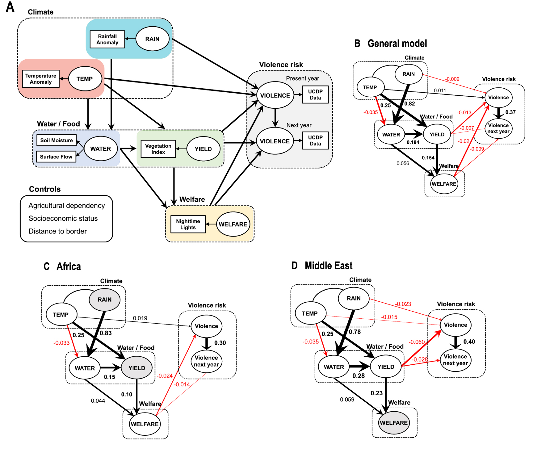
When applying the SEM to both regions together [general model] (figure 2(B)), yield and economic welfare had the strongest effect on present-year violence risk. Increases in yield and welfare reduced the chance of violence in both present and following year, while warming increased the risk and rain decreased this risk.
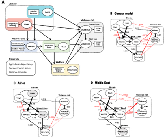
Figure 2. Structural equation models showing causal effects on conflict risk. (A) The conceptual model. Models were applied to (B) Africa and Middle East together (general model), and to (C) Africa and (D) Middle East separately. Factors not affecting present-year violence are colored gray. Numbers alongside arrows indicate the standardized direct effects, with the color of the arrow indicating its sign (black for positive; red for negative) and width indicating its importance in the model. Constructs in our SEM are indicated by ovals while indicators are shown as rectangles. Only significant effects at P < 0.05 are shown.
Download figure:
Standard image High-resolution imageWhile these results are in accordance to previously reported by others [19, 21, 38], unexpected complex climate-conflict links were revealed when SEMs were applied to each region separately (figures 2(C) and (D)). Warming increased the risk of violence in Africa (figure 2(C))—similar to the general model—but unexpectedly decreased this risk in the ME (figure 2(D)). There was no effect of rain and yield on conflict risk in Africa and no effect of welfare in the ME. But there was a weak, though significant (P < 0.05), indirect negative effect of rain on the risk of conflicts in Africa (table 1), which was, surprisingly, through the effect of water availability on welfare and not through yield (figure 2(C)). This may be in part because satellite-based estimates of yield have limited skill in some conflict-prone African regions (figures S3 and S4), but could also be due to a more complex link between rainfall, yield, and violence than that drawn by our model. In all models, the risk of violence was greater in places where conflict already occurred in the previous year (figures 2(B) to (D)), which likely indicates the roles of political instability and historic background on such conflicts.
4.2. A non-linear response of conflict to warming
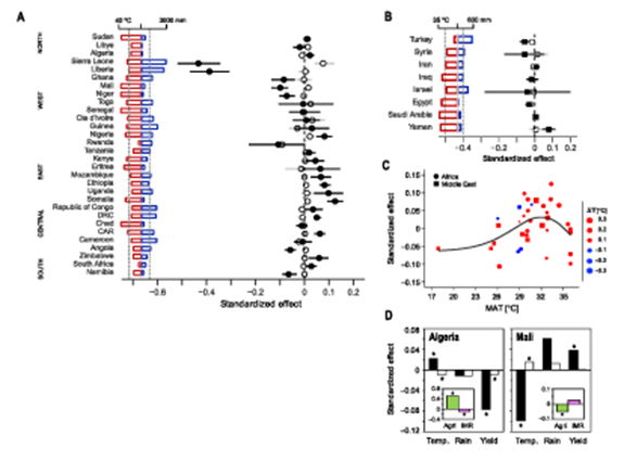
To examine the generality of the contrasting effects, we further applied the SEMs per country. After analyzing the countries with enough conflicts to produce a statistically significant model (table S4), we found that not only ME countries, but also some African countries—particularly West African—had a negative, direct temperature effect on violence risk (figure 3(A)). This negative direct temperature effect was in spite of the fact that some of these countries are warmer than those showing a positive effect [e.g. East African countries], which would theoretically make them more vulnerable to heat-induced violence [23]. In general, the country data show a non-linear relationship between the warming effect—i.e. the standardized direct effect of temperature anomaly on conflict risk—and the mean temperature conditions across countries, with a peak response at around 32 C (figure 3(C)). Countries with lower and higher mean annual temperatures (MAT) tend to exhibit lower effects of temperature anomalies on the risk of violence, with even negative effects in some cases.
Figure 3. Contrasting effects of temperatures on conflict risk. Direct (close symbols) and indirect (open symbols) standardized effects of temperature on the risk of conflict from SEMs in (A) African and (B) Middle Eastern countries. Mean annual temperature and rainfall over 1992–2012 are shown. Effects with bars not crossing the vertical line in (A) and (B) are considered significant at P< 0.05. (C) The standardized direct effect of temperature vs. local temperature conditions expressed as the mean annual temperature [MAT]. Each symbol in (C) is a single country (Sierra Leone and Liberia are excluded for clarity), with the size indicating the average temperature change [ΔT] for the period of analysis and the line in depicting the nonparametric regression with corresponding confidence interval. (D) The standardized direct (black) and indirect (white) effects of temperature, rain, and yield on conflict risk in Algeria and Mali. Inserts in (D) show the effects of agricultural dependence and infant mortality rate (IMR) in Algeria and Mali. Asterisks denote significant effects at P < 0.05.
Download figure:
Standard image High-resolution image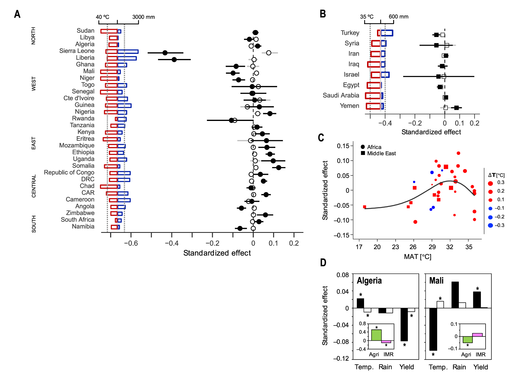
An example of the latter is Sierra Leone and Liberia, which had the strongest effects, with a standardized negative effect of −0.43 and −0.39, respectively (figure 3(A)). These two countries are characterized by extremely warm and humid conditions, with high temperatures and large amounts of rainfall year-round (3000 mm y−1). Contrary to the GAM, which suggests that uncomfortable environmental conditions increase violent perceptions [3], in this case uncomfortable extreme weather conditions [extra warming in already warm, humid countries] seemed to decrease the risk of violence.
Some experimental studies suggested that physical aggression may have a rather complex, curvilinear response to heat [62–64]. Aggression was shown to increase with temperature rise, but decrease at excessive heat in several experimental settings, particularly when other negative-affect-producing factors are present [64]. The explanation given for this is that it is the urgent 'need' to escape or minimize discomfort that overcomes tendencies to aggressive behavior [65]. Taking this to Sierra Leone and Liberia, a further increase in temperature resulting in extremely unpleasant conditions might have increased discomfort and reduced the level of engaging in violence through such 'escape' mechanism. In this context, the RAT—suggesting that people interact more under pleasant conditions, which lead to more opportunities for violence—may be another possible explanatory mechanism [18].
The positive and negative temperature effects in Yemen and Turkey (figure 3(B)) suggest that GAM might be the primary mechanism in the ME rather than the RAT. The contrasting sign effect may be explained by a relaxation mechanism in which a decrease in unpleasant conditions—being warming in a cold area [Turkey] or cooling in a warm area [Yemen]—reduces the chance of violence [66]. This does not necessarily contradict the abovementioned 'escape' theory because warm and humid conditions in both Turkey and Yemen are more tolerable than in Sierra Leone and Liberia (figures 3(A), (B)).
4.3. Climate effects in the context of geography and ethnicity
To further show how complex this climate–conflict link may be, we focus on two cases—Algeria and Mali. Algeria is the largest country in Africa, with an economy relying heavily on energy exports. Though Algeria's government has promoted agricultural development, yield is highly unstable due to climate variability [67]. This instability is likely to promote violence, particularly in agriculture-dependent areas as shown from our results (figure 3(D)). The contrasting indirect [negative] and direct [positive] effects of temperature in Algeria are likely due to a positive temperature effect on yield and a direct adverse influence of heat, which may be explained by the GAM. In contrast, the influence of yield on violence risk was positive and significantly smaller in Mali [50% smaller than in Algeria]. This is in spite of the fact that Mali's economy is more centered on agriculture than Algeria [68]. Moreover, the positive yield effect was limited to the northern part of Mali, which is less agricultural than its southern [and central] part (insert in figure 3(D)).
Putting this in context, we know that most conflicts in Mali during the period of analysis were intra-state conflicts between the government and the Tuareg nomadic inhabitants living in the northern part of the country. Because our analysis is limited to small-scale conflicts, the non-state, inter-group aspects of the Tuareg conflict, which occur primarily in the northern, less agricultural part of the country, is well noted (figure 1(A)) [68]. The Tuaregs are primarily pastoral and as such continuously compete for scarce resources between pastoral groups and with the few crop farmers and settled villagers in the north [68]. Tuareg conflict is believed to be an example of a resource conflict driven by climatic changes [69] and the positive effect of yield on violence risk in our SEM is likely a reflection of this struggle, with periods of increased yield in the northern region being a potential driver of ethnic tension and inter-group violence.
These contrasting complex links in Algeria and Mali imply that the climate–violence linkage should be investigated in the context of historical, geographical and ethnical backgrounds of each location rather than as a general cross-sectional analysis. Such an approach can shed light on contrasting effects of climate.
5. Concluding remarks
Our findings reveal previously unreported effects of climate on risk of conflict outbreak. More specifically, contrasting effects of temperature were detected at a regional scale and in numerous countries in Africa and the ME. Importantly, temperature and rainfall direct effects on conflict risk seem to be stronger than any indirect effect through resources such as water availability and agricultural production (figure 3 and table 1). This could mean one of three things: that climate affects violence mostly through psychological and/or interactive mechanisms [e.g. GAM and RAT [17, 18]]; that indirect effects depend on aspects of climate variability that we have not considered [70]; or that underlying mechanisms in which resource scarcity or conflict-relevant abundance patterns affect violence are more complex than those modeled by our SEMs.
As in previous studies [21], the use of explicit controls affected the strength of the climate effect in our SEMs [i.e. the difference between total and direct effects in table 1], in our case by up to 46%. This was important enough to expose indirect rain effects in Africa (table 1). It is important to note that the SEMs, although statistically significant (table S4), confirming the validity of the a priori hypothesis, had very little predictive power [with 1st and 3rd quantiles being 1.6% and 11%, respectively, across countries] (table S5). This means that although our SEMs did confirm impacts of climate on armed conflicts by effectively quantifying its direct and indirect effects, these effects were relatively small compared to unobserved factors like political, ethnic and likely other unaccounted socioeconomic factors. These were only partly considered in our analysis, due to the difficulty to account for such factors at a grid-cell level, in the form of next-year violence risk, which was shown to be greatly affected by present year violence (explaining between 10% and 16% of the variance, at the continental level; figures 2(B) to (D)).
Our results demonstrate that no single proposed climate–conflict mechanism can alone explain the empirical patterns that underlie the climate–conflict linkage across contrasting regions or countries, and that this linkage is more complex than some analyses have previously suggested [21]. We conclude that extreme caution should be exercised when attempting to explain or project local climate–violence relationships on the basis of a single, generalized theory. Large-scale cross-sectional studies can be useful for identifying general associations and trends, but an appropriately scaled and structured analysis is required to explain and, potentially, address climate–violence risk factors in geographic context.
Acknowledgments
Authors thank C Helman for helping to organize the data for the analyses, A Mussery for helping to organize the SEMs results in the SM, and two anonymous reviewers for insightful comments. D Helman was a USA-Israel Fulbright Post-Doctoral Fellow at Johns Hopkins University 2018/19. C Funk is supported by the U.S. Geological Survey Drivers of Drought program and the U.S. Agency for International Development's Famine Early Warning Systems Network.
Data availability statement
The data that support the findings of this study are available upon reasonable request from the authors.