Machine learning assisted hybrid models can improve streamflow simulation in diverse catchments across the conterminous US

Similar to Kratzert et al (2018), we also select 531 CAMELS-US catchments which have no discrepancies in basin characteristics and have better model performance to train and compare different ML models. These CAMELS-US catchments have long-term streamflow observations, are minimally impacted by human activities, and cover a wide range of hydroclimatic conditions across the Conterminous US. For each catchment, we obtained 1980–2010 observed daily precipitation, minimum and maximum daily temperature, solar radiation and vapor pressure as predictors for ML streamflow training and testing. These five meteorological predictors are spatially aggregated at each catchment from the 1 km resolution Daymet data set (Thornton et al 2017). The streamflow observations are obtained from US Geological Survey National Water Information System. In addition to the observed streamflow time series, we also obtained simulated SAC streamflow from Newman et al (2014) as the PB model output analyzed in this study. The SAC model was forced by the same catchment-averaged Daymet data for the period 1980–2010 and calibrated against 1980–1995 daily streamflow using the shuffled complex evolution global optimization routine. For further details on SAC model configuration and calibration, the readers are referred to Newman et al (2014).

To understand the relationship between model performance and catchment features, we obtained characteristics related to: (1) climate, (2) topography and soil, (3) hydrology, (4) geology, and (5) vegetation for the same 531 catchments from Addor et al (2017). These catchment characteristics were not used in the SAC model calibration, but provided as a complementary dataset to facilitate comprehensive multivariate catchment-scale assessments. The topographic characteristics (e.g. elevation and slope) were retrieved from Newman et al (2014). Climatic indices (e.g. aridity and frequency of dry days) and hydrological signatures (e.g. mean annual discharge and baseflow index) were computed using observations provided by Newman et al (2014). Additional soil (e.g. porosity and soil depth), vegetation (e.g. leaf area index and rooting depth), and geological (e.g. geologic class and subsurface porosity) characteristics were derived by Addor et al (2017). The complete list of selected catchment characteristics, as well as details on the methods and data used to compute them, is provided in Supplementary Table S1. The catchments characteristics are summarized in Table S2. Further details on the CAMELS-US catchment characteristics are provided in Addor et al (2017).

A LSTM network is a special type of RNN that can store and regulate information over time and thus particularly suitable for simulating memory effects of meteorological inputs on streamflow (Shen 2018). This is important in streamflow simulation because some catchment processes such as snow accumulation, soil water storage and groundwater contribute significantly to streamflow at long time scales (Tague et al 2008, Pellicciotti et al 2010, Carey et al 2013). The temporal memory effect is simulated by the combined use of cells and gates in LSTM (Hochreiter and Schmidhuber 1997), where the cells act as memory units and the gates control the information flow. Also, as opposed to the conventional RNN, LSTM does not have a problem with exploding and/or vanishing gradients, which allows it to efficiently map long-term dependencies between input and output sequences (Gers et al 2000).

Given an input sequence with T time steps, x = [x[1],...,x[T]], where x[t] is a vector containing input features at any time step t, the following equations describe the forward pass through the LSTM:

$$\begin{equation}i\left[ t \right] = \sigma \left( {{W_i}x\left[ t \right] + {U_i}h\left[ {t - 1} \right] + {b_i}} \right)\end{equation} \tag{ 1 }$$

$$\begin{equation}f\left[ t \right] = \sigma \left( {{W_f}x\left[ t \right] + {U_f}h\left[ {t - 1} \right] + {b_f}} \right)\end{equation} \tag{ 2 }$$

$$\begin{equation}o\left[ t \right] = \sigma \left( {{W_o}x\left[ t \right] + {U_o}h\left[ {t - 1} \right] + {b_o}} \right)\end{equation} \tag{ 3 }$$

$$\begin{equation}g\left[ t \right] = {\text{tan h}}\left( {{W_g}x\left[ t \right] + {U_g}h\left[ {t - 1} \right] + {b_g}} \right)\end{equation} \tag{ 4 }$$

$$\begin{equation}h\left[ t \right] = o\left[ t \right] \odot {\text{tan h}}\left( {c\left[ t \right]} \right)\end{equation} \tag{ 5 }$$

$$\begin{equation}c\left[ t \right] = f\left[ t \right] \odot c\left[ {t - 1} \right] + i\left[ t \right] \odot g\left[ t \right]\end{equation} \tag{ 6 }$$

where i[t], f[t] and o[t] are the input, forget, and output gates controlling the flow of memory, g[t] and h[t] are the cell update and recurrent inputs, c[t] represents the cell state, $\left( {{W_i},{\text{ }}{W_f},{\text{ }}{W_o},{W_g}} \right)$, $\left( {{U_i},{\text{ }}{U_f},{\text{ }}{U_o},{U_g}} \right)$ and $\left( {{b_i},{\text{ }}{b_f},{\text{ }}{b_o},{b_g}} \right){\text{ }}$are the input, recurrent and biases weights, σ(⋅) is the sigmoid function, tanh (⋅) is the hyperbolic tangent function, and ⊙ is element-wise multiplication. Based on the above formulation, the cell states (c[t]) characterize the memory of the system and can be modified by the forget gate (f[t]) to delete state memory, or by the input gate (i[t]) and cell update (g[t]) to add new information. In the latter case, the cell update is seen as the information that is added and the input gate controls which cells information is added. Finally, the output gate (o[t]) controls which information, stored in the cell states, is outputted. For a more detailed description, the readers are referred to Kratzert et al (2018).

In addition to the PB model output from Newman et al (2014), we trained and tested three models to simulate daily streamflow. First, a stand-alone LSTM that simulates streamflow based on time series of the five Daymet variables (i.e. precipitation, maximum and minimum daily temperature, solar radiation and vapor pressure). Second, a hybrid LSTM (Hybrid1) that simulates streamflow based on time series of the five Daymet variables and also the PB model output. Third, a hybrid LSTM (Hybrid2) that simulates the PB model residual (i.e. simulated SAC streamflow minus observed streamflow) based on time series of the five Daymet variables. The estimated residual is then added to the PB model output to generate the corrected streamflow.

Since the SAC model is calibrated using daily data from 1980–1995, we use the same time period to train all three ML models to maximize the Nash–Sutcliffe efficiency (NSE; Nash and Sutcliffe 1970). NSE can be computed as:

$$\begin{equation}NSE = 1 - \frac{{\mathop \sum \nolimits_{t = 1}^T \left( {Q_m^t - Q_o^t} \right)}}{{\mathop \sum \nolimits_{t = 1}^T \left( {Q_o^t - \overline {{Q_o}} } \right)}}\end{equation} \tag{ 7 }$$

where $\overline {{Q_o}}$ is mean of observed streamflow, $Q_m^t$ is the modeled streamflow, and $Q_o^t$ is the observed streamflow at time t. NSE varies from -∞ to 1 with 1 representing the perfect match and negative values representing worse results than the mean value. We tested the model performance using 2000–2010 observed daily streamflow. For these three models (i.e. LSTM, Hybrid1 and Hybrid2) we used the same network architecture with 20 hidden states, 0.1 dropout rate, and 365 d as an input sequence with a single fully connected LSTM layer. The determination of the network hyperparameters have a significant influence on simulation results. We set the input sequence length of 365 d in order to capture the hydrological dynamics of a full annual cycle. We used a single layer network with relatively small hidden states plus dropout in order to avoid overfitting and enable the network to have a robust feature learning. We determined the specific values of hidden states and dropout through a number of test runs across different US catchments. The architecture used in this study proved to work well for these catchments and was therefore chosen to be applied here without further tuning.

To study the catchment features associated with the enhanced (or deteriorated) performance of the ML model with respect to the original PB model, we compute the change of NSE (e.g. ΔNSE_ML-PB = NSE_ML—NSE_PB) during the validation period (2000–2010). We then perform a regression analysis of ΔNSE using the catchment characteristics as predictors through the Random Forest algorithm (Breiman 2001). By using the Random Forest algorithm, we can rank the non-linear and non-parametric importance of each covariate to identify the dominant catchment characteristics associated with PB model performance using the dropout loss approach (Strobl et al 2007, Grömping 2009). Dropout loss is the decrease in random forest algorithm accuracy when a single covariate value is randomly shuffled. This procedure breaks the relationship between covariate and classification target, thus the decrease in accuracy score is indicative of how much the model depends on the tested predictor (i.e. higher dropout for more important variable). In general, an important covariate has a response function that displays interpretable features such as tipping points, well defined minima/maxima, or a slope (Murdoch, 2019). In contrast, variables with flat response functions (i.e. no change in NSE over the range of target variable) are relatively unimportant (Breiman 2001, Schwalm et al 2017). Accumulated local effect (ALE; Apley 2016) plots based on the Random Forest algorithm can visualize this relationship between explanatory covariates and the probability of superior model performance. ALE gives the conditional effect of a covariate on the response variable and can get the isolated effect of each covariate even in the presence of correlation within covariates. Further details of dropout loss and ALE computations are provided in the supplementary information.

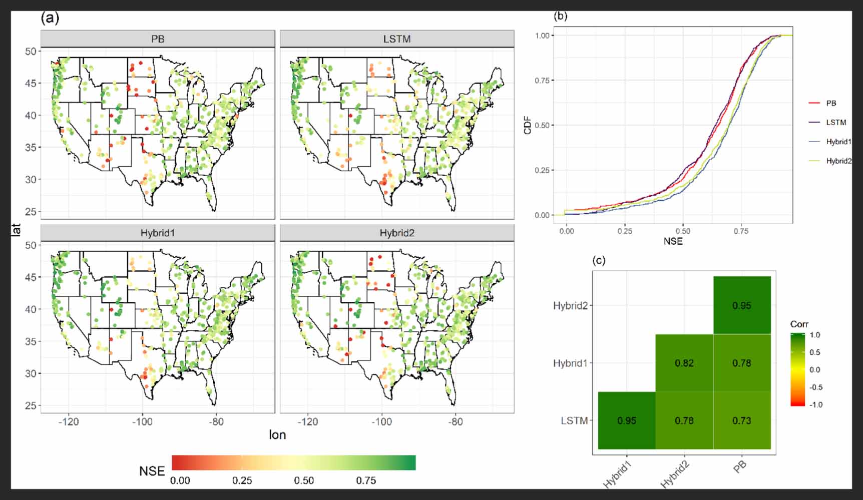
Figure 1 describes various aspects of model performance as determined by NSE of the four tested models (PB, LSTM, Hybrid1 and Hybrid2). The spatial patterns of NSE across the four models are broadly similar. Weaker model performance is found across the Great Plains (in and around the states of South Dakota and Nebraska) and in the arid catchments in Texas and Arizona, where both LSTM and Hybrid1 models show comparatively higher NSE than PB and Hybrid2. On the other hand, all four models show stronger performance in the eastern and western US (figure 1(a)). The cumulative distribution functions (CDFs) of NSE values in figure 1(b) indicate that both hybrid models (Hybrid1 and Hybrid2) exhibit higher NSE values than the stand-alone PB and LSTM models, suggesting the overall enhanced performance through PB-ML hybrid modeling. Also, Hybrid1 is more correlated to LSTM (figure 1(c)), while Hybrid2 is more correlated to PB. The relatively higher correlation between LSTM and Hybrid1 (PB and Hybrid2) might be due to similar performance in the Great Plains and the arid catchments in Texas and Arizona.

Zoom In Zoom Out Reset image size

We further explore the ΔNSE of ML-assisted models (LSTM, Hybrid1 and Hybrid2) in figure 2. In figure 2(a), we classified all catchments by the original PB performance into four categories (NSE_PB ≤ 0, 0 < NSE_PB < 0.5, 0.5 ≤ NSE_PB ≤ 0.75 and NSE_PB > 0.75) and analyzed the spread of ΔNSE_LSTM-PB, ΔNSE_Hybrid1-PB, ΔNSE_Hybrid2-PB through boxplots. Overall, the standalone LSTM performs better for catchments with poorer PB performance (NSE_PB ≤ 0.5), but cannot outperform PB if the PB performance is already high (NSE_PB > 0.5). Both hybrid models can provide overall improvement but with different patterns. Hybrid1 that uses the PB simulated streamflow as the LSTM input behaves more similar to the standalone LSTM, while Hybrid2 that uses the PB model residual as the LSTM input show more uniform but smaller enhancement across all catchments. It is worth mentioning that all ML-assisted models show highest improvement where the PB model has failed (i.e. catchments where NSE_PB < 0). However, as the PB model performance becomes better, even though there is a positive improvement in ML models, the magnitude of ΔNSE decreases. Among the ML models, Hybrid1 provides the highest median improvement over a wide variety of catchments across all four categories. Whereas, the standalone LSTM model has better performance than Hybrid2 when NSE_PB ≤ 0.5, and vice versa.

Zoom In Zoom Out Reset image size

The probability density functions (PDFs) of ΔNSE values are shown in figure 2(b), which indicate that the performance of Hybrid1 and Hybrid2 are overall higher than PB. It is interesting to see that there are fewer number of catchments with ΔNSE < 0 in Hybrid2 (comparing to the higher number of catchments with ΔNSE < 0 in LSTM and Hybrid1). This can also be observed in the spatial map in supplementary figure S1, which can be found online at https://stacks.iop.org/ERL/15/104022/mmedia, where Hybrid2 has a relatively smaller number of catchments with ΔNSE < 0. This suggests the different effects of these two hybrid modeling approaches. While Hybrid1 may provide greater improvement, it may also lead to undesired deterioration in some catchments. Whereas, Hybrid2 can provide very consistent but weaker improvement. Based on the results, it seems that the most beneficial applications of PB-ML enhancement are for catchments with poorer PB performance (NSE_PB ≤ 0.5) through the Hybrid1 approach. In such cases, both standalone LSTM and Hyrbird1 can largely improve the performance of streamflow simulation, suggesting the possibility of missing model processes captured by ML. Although both hybrid approaches can also improve streamflow simulation for catchments with better PB performance (NSE_PB > 0.5), the improvement may be limited and could lead to undesired deterioration. These factors should be considered when evaluating the necessity to conduct streamflow modification through hybrid PB-ML modeling.

Our next step is to understand what catchment features have the strongest influences on hybrid model performance. For this purpose, we assessed the changes in model performance of Hybrid1 with respect to the PB model (ΔNSE_Hybrid1-PB) as well as to the standalone LSTM model (ΔNSE_Hybrid1-LSTM). Investigating these two variables would shed light on where hybrid model might be advantage/disadvantage. We use dropout loss and conditional dependency to identify important catchment characteristics and further visualize their relationships with model performance. We also conducted similar analysis for Hybrid2 but found that the change of Hybrid2 performance do not correlate to catchment characteristics. Therefore, the results of Hybrid2 are not showed. Overall, Hybrid1 performs better than Hybrid2 in catchments with higher aridity, elevation and baseflow. Whereas, Hybrid2 performs better in catchments with higher precipitation, streamflow and high flow (supplementary figure S4).

Using dropout loss, in figure S2, we show that climate, soil and topography, and hydrologic characteristics have stronger effects on the change of model performance of Hybrid1 with respect to PB (ΔNSE_Hybrid1-PB). In figure 3 we plot the accumulated local effect plots which visualize the contribution of the dominant catchment characteristics identified by dropout loss. As evident from figure S2, snow fraction has the highest dropout loss indicating that it is one most significant factor. Figure 3 highlights that with increasing snow fraction and elevation, the probability of better Hybrid1 performance increases. This suggests potential issues of PB model's snow accumulation and ablation module (SNOW-17; Anderson 2006) for the applications on these CAMELS-US sites. In particular, we believe that the superior performance of Hybrid1 may be attributed to its ML component, which better captured the time lagged snow accumulation and melting process (Kratzert et al 2018).

Zoom In Zoom Out Reset image size

We can also see that hybrid model improves the performance in regions of low precipitation and high aridity indicating their ability to capture the complex arid climate hydrology. Hybrid models have exhibited better performance in regions with high baseflow index. Factors that promote infiltration and recharge of subsurface storage will increase baseflow index, while factors associated with higher evapotranspiration will reduce baseflow index (Bloomfield et al 2009, Konapala and Mishra 2020). Therefore, in these catchments, the hybrid model was able to capture the slow groundwater drainage component which results in high baseflow index that might not be well represented in the PB model. It is interesting that ML models may distinguish these catchments based on data alone. This strength of LSTM was also reported by Kratzert et al (2019). It is also important to understand that the performance of hybrid model does decrease with low flow characteristics of duration and frequency. With the increase in low flow duration and frequency, there will be more irregular streamflow pulses which increases the complexity of streamflow series (Vogel and Fennessey 1994, Smakhtin 2001). Therefore, ML may not capture such complicated streamflow pattern. In addition, as the streamflow timing (i.e. half flow date) of the catchments shifts to end of water year the hybrid model performs better.

In figure 4, we show the functional relationship of top ten dominant catchment characteristics (figure S3) which have stronger effects on the change of model performance of Hybrid1 with respect to the standalone LSTM (ΔNSE_Hybrid1-LSTM) through accumulated dependence plots. The results are quite different than figure 3, in which stronger effects are found for vegetation, climate, hydrology, and soil and topography features. As evident from figure S3, the 99th percentile root depth has the highest dropout loss, and figure 4 highlights that lower 99th percentile root depth would result in higher ΔNSE_Hybrid1-LSTM. Lower root depth indicates less infiltration and more water available for runoff and evaporation. Therefore, the hybrid model was able to capture this relationship better than the standalone LSTM model. Also, similar to figure 3, the hybrid model performs better than the LSTM model in arid, high elevation, low precipitation and snow dominant catchments. This suggests that the hybrid model may overcome the deficiencies in both PB and standalone LSTM models in case of these variables. However, unlike figure 3, we find that the hybrid model performs significantly better than the LSTM model in catchments with low magnitude of runoff ratio, streamflow and Q95. This suggests that the hybrid model may better represent the high streamflow generation mechanism that may not be well captured in either of the PB and standalone LSTM models. Finally, hybrid models perform better with respect to standalone LSTM models in catchments with less forest area fraction and vegetation.

Zoom In Zoom Out Reset image size