


Abstract
Prediction of high latitude response to climate change is hampered by poor understanding of the role of nonlinear changes in ecosystem forcing and response. While the effects of nonlinear climate change are often delayed or dampened by internal ecosystem dynamics, recent warming events in the Arctic have driven rapid environmental response, raising questions of how terrestrial and freshwater systems in this region may shift in response to abrupt climate change. We quantified environmental responses to recent abrupt climate change in West Greenland using long-term monitoring and paleoecological reconstructions. Using >40 years of weather data, we found that after 1994, mean June air temperatures shifted 2.2 °C higher and mean winter precipitation doubled from 21 to 40 mm; since 2006, mean July air temperatures shifted 1.1 °C higher. Nonlinear environmental responses occurred with or shortly after these abrupt climate shifts, including increasing ice sheet discharge, increasing dust, advancing plant phenology, and in lakes, earlier ice out and greater diversity of algal functional traits. Our analyses reveal rapid environmental responses to nonlinear climate shifts, underscoring the highly responsive nature of Arctic ecosystems to abrupt transitions.
Export citation and abstract BibTeX RIS
The discovery of abrupt climate change events in Greenland ice cores altered the paradigm that climate change operates slowly and gradually, revealing major changes in less than a decade in temperature, atmospheric circulation and precipitation (Johnsen et al 1992, Alley et al 1993, Mayewski et al 1993). As greenhouse gases continue to rise, there is the persistent, looming possibility of abrupt and highly disruptive climate shifts of uncertain magnitude in the future (Pittock 2008). The inherent threats of climate state changes for humans and ecosystems not only include the uncertainty of the magnitude of these changes until they actually happen, but also the uncertainty of the nature of ecosystem response to this forcing. Quantifying ecosystem response to rapid shifts in climate has been difficult because of the influence of multiple drivers, the insufficient period of systematic environmental monitoring relative to climate change versus climate variability, and the relatively coarse temporal resolution of paleoecological records (Burkett et al 2005, Bestelmeyer et al 2011, Williams et al 2011). This lack of clarity hinders prediction of ecosystem response to rapid climate change. Determining how to anticipate, avoid, and manage abrupt climate change has been identified as one of the five grand challenges to global sustainability (Reid et al 2010), raising the need to better understand ecosystem response to rapid climate shifts.
Even under gradual climate change, ecosystems exhibit nonlinear responses (Burkett et al 2005, Williams et al 2011), hence nonlinearity in extrinsic drivers of ecosystem change may further complicate ecosystem dynamics, and we are only beginning to understand these changes (Bestelmeyer et al 2011, Williams et al 2011) and the potentially adverse consequences of abrupt transitions between ecosystem states (Scheffer et al 2001). Ecological shifts are driven by thresholds in ecological systems (intrinsically forced), in the climate system (extrinsically forced), or both. While less common, extrinsically forced ecological shifts are apparent in paleoecological records, particularly after large magnitude climate changes, such as warming by 9 °C in less than 70 years during the Bølling-Allerød 14 670 years ago or by 15 °C over a few decades after the Younger Dryas 11 700 years ago (Williams et al 2011). Pollen records indicate vegetation shifts 30–200 years after these large magnitude, abrupt climate changes. What remains less clear is the nature and rate of environmental response to smaller magnitude yet significant climate shifts.
With the Arctic warming at a rate two to three times that of the global average over the past 150 years (IPCC 2013), climate forcing is the dominant driver of ecosystem changes in this region (Smol et al 2005, Post et al 2009, Schuur et al 2015). Across the Arctic, environmental effects of climate change spanning the last 150 years include increased turnover in aquatic species composition, extended growing season length with consequences for greening and shrubification, and enhanced permafrost thaw driving changes in carbon and nutrient cycling (Smol et al 2005, Post et al 2009, Schuur et al 2015). However some of the most pronounced changes have occurred with recent, rapid warming events, leading to record lows in Arctic sea ice extent and the Greenland Ice Sheet (GrIS) mass balance (Parkinson and Comiso 2013, Tedesco et al 2013). This raises questions about how sustained shifts in climate forcing may alter terrestrial and freshwater ecosystems, and what adverse consequences may arise as a result.
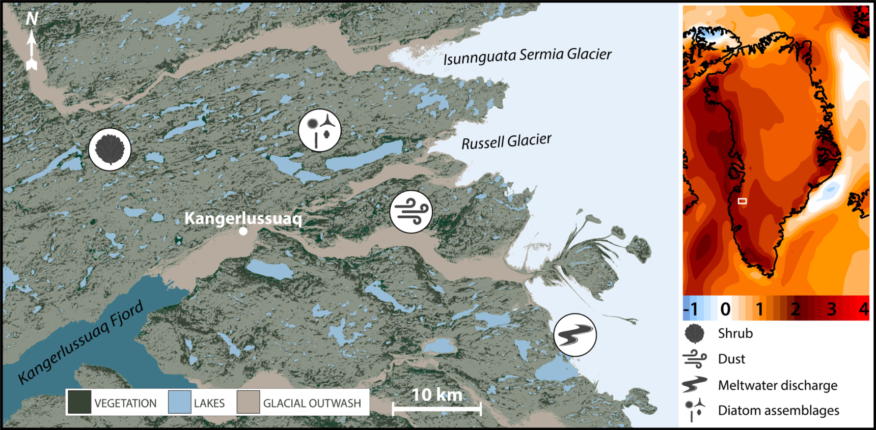
Greenland provides perhaps the most striking recent example of rapid climate change in the Arctic, where mean annual air temperatures between 2007 and 2012 were 3 °C higher than the 1979–2000 average (Mayewski et al 2014). In contrast to much of the Arctic, the area of Kangerlussuaq, West Greenland, exhibited no discernible warming during most of the 20th century but started warming rapidly in 1995 (Hanna et al 2012) (figure 1). Given that much of the Arctic was warming from ∼1950 (Kaufman et al 2009), prior to the initiation of systematic environmental monitoring, the more recent rapid warming in the Kangerlussuaq area provides a unique opportunity to assess the range of ecological response to rapid temperature increase.

Figure 1. The paraglacial landscape around Kangerlussuaq, West Greenland. Legends indicate key landscape features (bottom left) and focal environmental responses (lower far right). Inset depicts recent warming in Greenland as indicated by temperature anomaly (°C, indicated in color scale), annual 1995–2015 minus 1979–1994, based on European Reanalysis Interim (ERA-Interim) with map created using Climate Reanalyzer; location of Kangerlussuaq region indicated by white box.
Download figure:
Standard image High-resolution imageHere we assess the response of environmental conditions and biological communities to nonlinear changes in climate in West Greenland using long-term monitoring records and paleoecological reconstructions. Temporal extents of three of the environmental time series are extended using models developed from monitoring data. In addition to climate and environmental time-series analyses, we assessed chemical and biotic responses of lakes before and after the most recent warming event. This additional analysis of lakes was included because lakes are integrators and thus act as sentinels of change to their surrounding environment (Williamson et al 2009). We hypothesized that with nonlinear changes in temperature and precipitation, most environmental variables would exhibit delayed and/or linear responses, consistent with previous research (Bestelmeyer et al 2011, Williams et al 2011).
Methods
Climate
We conducted exploratory analyses of regional and local climate. Time series were analyzed over annual and seasonal (DJF, MAM, JJA, SON) scales. Mean air temperatures were also analyzed by month because of a significant (p < 0.05) result during JJA. These are three months that capture the summer season at lower latitudes, but in the Arctic, June captures part of the spring season. Results of all analyses are provided in supplementary information, available online at stacks.iop.org/ERL/14/074027/mmedia (figures S1–5).
Greenland Blocking Index (GBI)
The atmospheric high-pressure region that forms over Greenland (described by the GBI) affects regional air temperature and precipitation. Historical trends in GBI have been determined from direct measurements of synoptic pressure taken since 1851 (Hanna et al 2016). The monthly GBI record used in this study is based on a homogenization of the Twentieth Century Reanalysis version 2c product (20CRv2c) spliced with NCEP/NCAR Reanalysis GBI. The GBI record covers the period 1851–2015. For the common period, 1948–2015, all monthly correlation coefficients between the two unspliced reanalysis time-series are above 0.92. Before the splicing, seven potential artifactual breakpoints were corrected for by homogenization of the 20CRv2c data (Hanna et al 2016). The unspliced NCEP/NCAR Reanalysis product is used after 1948, while the spliced GBI time-series is used before 1948.
Atmospheric air temperature
Monthly air temperature data for Kangerlussuaq were obtained from WMO Station 04231, which has recorded hourly air temperature since 1942. The station was run under the auspices of the US Air Force from 1942 to 1972 and the Danish Meteorological Institute (DMI) from 1973 to present. The location of the meteorological station moved in 1973 but both ran concurrently for a number of years and the hourly temperatures at the two sites have a very high correlation (e.g. 1973, r = 0.99 (n = 1143); 1985, r = 0.99 (n = 1143)). Breakpoint analyses for all months for the full record (1942–2015) are provided in figure S4. Breakpoint analyses for all months using only the DMI record (1973–2015) are provided for comparison in figure S5 and demonstrate similar results.
Precipitation
Precipitation has been measured at the DMI 04231 station since 1976 using a Hellmann-type gauge. We used the monthly precipitation record covering the period 1976–2012, which has been corrected for systematic biases related to wetting loss and wind-induced undercatching (Mernild et al 2015).
Environmental response time series
To assess ecosystem responses, a combination of paleoecological and contemporary field observations, remote sensing and modeling were used. For modeled data, we: (1) indicate the time frame of observations used in model development and correction but only use the modeled data in statistical analyses; (2) compare observed versus modeled data here or in cited literature. Time frames covered in each series vary. We analyzed time series of GrIS discharge (Watson River; modeled 1979–2014 with corrections applied based on measurements spanning 2006–2015 (Mernild et al 2018)), GrIS outwash plain dust (observed 1973–2015 (Bullard and Mockford 2018), paleorecord 1860–2011), plant phenology (timing of 50% plant species emergence; observed 2002–2011, modeled 1979–2012 Kerby and Post 2013), Betula nana shrub ring chronology (Ring Width Index derived from measurements of multiple individuals between 1941 and 2013 Gamm et al 2018), lake ice out (Hundesø Lake; modeled 1973–2015 based on observed 1992–2015 on the ground and/or via satellite imagery), and lake sedimentary diatom fossils (three sediment cores spanning ∼1900 to 2010 or later, community change analyzed with principal components analysis).
GrIS discharge
The Watson River catchment covers approximately 12 000 km2 of the western sector of the GrIS (Lindbäck et al 2015) and c. 575 km2 of proglacial area (Yde et al 2014). We simulated annual runoff for 1979/80–2013/14 using the SnowModel software package and the ERA Interim reanalysis product as atmospheric forcing (Mernild et al 2018). Atmospheric variables from ERA Interim reanalysis, which are used as forcings in SnowModel simulations, are downscaled and adjusted to the ice sheet topography using a 5 km horizontal grid DEM. SnowModel also uses albedo and sublimation, as well as the flow residence time and flow velocities, which depend on travel distance, glacier surface slope and density of surface depressions, porosity and temperature of the snow and ice matrix, temporal development of the snowpack, and temporal changes in the size of the supra- and subglacial drainage channels. Modeled runoff was adjusted to observed runoff (van As et al 2018). Observed runoff from Watson River was monitored at a hydrometric station located close to the river outlet into the fjord Kangerlussuaq (Hasholt et al 2013), and was derived from a stage-discharge relation, where discharge was measured by a propeller current meter at low discharge and by float measurements and acoustic Doppler current profiler at high discharge. Data gaps in the observed runoff record were filled by applying an air temperature-based relation between runoff and air temperature measured at the DMI 04231 station. Modeled and observed records are compared in figure S6 (R2 = 0.99, RMSE = 11.4 × 10⁷).
Dust
GrIS outwash plain dust records include paleo records spanning 1860–2011 and an instrumental record spanning 1973–2015 (Bullard and Mockford 2018). The minerogenic flux in 210Pb-dated lake sediment cores, corrected for sediment focusing, is used as a proxy for the regional atmospheric dust loading (n = 55). This is a valid approach as the four lakes (SS901, SS903, SS904, SS16) used to calculate the regional average have limited if any inflow streams that might deliver minerogenic sediments that would compromise the use of lake mineral accumulation rate (minAR) as primarily reflecting atmospheric inputs. The dry mass accumulation rate was multiplied by the proportion of sediment that was determined to be inorganic (as the mass remaining after ignition at 550 °C). The carbonate fraction in the four lakes is minimal as they are too dilute to precipitate carbonate (Whiteford et al 2016) and diatom concentrations suggest that the biogenic silica fraction in the sediments is <5% and therefore can be ignored. The minAR was corrected for sediment focusing using the 210Pb flux method (Lamborg et al 2013) to make the results from an individual lake directly comparable; a LOESS smoother was then fitted to the combined profiles. For the modern dust record, WMO SYNOP Present Weather dust codes (07-09 and 30-35) recorded at Kangerlussuaq airport from 1973 to 2015 were used to calculate the dust storm index (DSI) for the area (n = 43) (O'Loingsigh et al 2014). The DSI weights different types of dust events according to their relative intensity, provides a composite measure of the changing frequency and intensity of dust events, and is calculated by:
where: DSI = dust storm index at n stations where i is the ith value of n stations for I = 1−n. In this case n = 1 (WMO Station 4231). SDS = Severe Dust Storm days (daily maximum dust codes 33-35), MDS = Moderate Dust Storm days (daily maximum dust codes 30-32) and LDE = Local Dust Event days (daily maximum codes 07-09).
Terrestrial plant responses
We examined two metrics of terrestrial plant response to climate: plant phenology and Betula nana growth. The terrestrial plant phenology (timing of 50% plant species emergence) record is based on observations in the Kangerlussuaq area from 2002 to 2011, used to model a time series spanning from 1979 to 2012 (n = 34) (Kerby and Post 2013). The model uses Arctic-wide sea ice extent (ASIE) from winter and early summer as the predictor of timing of 50% plant species emergence (R2 = 0.80; RMSE = 3.2); ASIE was a stronger predictor than any local weather, large-scale temperature or regional sea-ice cover metrics tested (R2 < 0.30 in all cases). Correlations between monthly ASIE and mean June temperatures in Kangerlussuaq were weak (Pearson's r ≤ ±0.20). Betula nana shrub ring chronology (Ring Width Index derived from measurements of multiple individuals) spans from 1941 to 2013 (n = 72) (Gamm et al 2018).
Lake ice out
The date of lake ice out in spring was modeled for the period 1973–2015 (n = 43) using the DMI weather station data and a record of ice out dates spanning from 1992 to 2015. The ice out record was constructed for a pair of lakes (Hundesø Lake and Lake SS85; Lat 66.98, Long −51.06) using a combination of satellite imagery, in situ thermistors, and direct observation on the ground. The inter-annual timing of ice out changes is one of the most coherent responses of lake ecosystems to climate, i.e. changes in the timing are highly synchronous across lakes in a region (Magnuson et al 2000). Between 1992 and 2015, ice out (i.e. date of final ice melt on lakes) was determined for 22 of the 24 years using satellite imagery (from Landsat 5, Landsat 7, Terra or Aqua satellites, depending on the year, time frame and cloud cover). These satellite observations of ice out were independently confirmed in four of the years by in situ thermistor readings (2002, 2003, 2005, 2007) and in an additional four years by on the ground observation (2000, 2011, 2013, 2014). Multiple linear regression was used to assess relationships among weather station data and ice out dates; the strongest model included only average May temperature (Ice Out Date = −3.167(mean May temperature) + 167.3; R2 = 0.62, RMSE = 7.15). This relationship was used to model ice out dates for 1973–2015. Modeled and observed records are compared in figure S7. Only the modeled dates were used in the breakpoint analysis. With the coherence of the ice out breakpoint with the mean June temperature breakpoint, we assessed whether mean May and mean June temperatures were correlated in the 1973–2015 weather station data, and found weak but significant correlation (Spearman's rank correlation ρ = 0.39, p = 0.01).
Sedimentary diatom assemblages
Diatom assemblages were determined in sediment cores from three lakes (SS15, SS901, SS903), spanning 1900 to at least 2011 (n = 11–29 per core). While there are many sedimentary diatom profiles available for this region (Perren et al 2009), those were collected in the late 1990s and hence only capture time prior to the recent period of climate change. Age models were determined using 210Pb profiles. Sediments were analyzed for diatom assemblages by digestion with hydrogen peroxide followed by microscopic counts (1000× magnification). Community change is quantified with Principal Components Analysis (PCA) axis 1 scores.
Pre-post breakpoint lake response
Contemporary changes in physical, chemical, and biological features of lake ecosystems were investigated more extensively given the sentinel (i.e. often earlier and more rapid than those of terrestrial systems) responses of lakes to climate change (Williamson et al 2009). Pelagic limnological measurements were conducted during summers over two time periods that bracket the summer GBI 2006 breakpoint (figure 2(D)): 1998–2002 (pre-breakpoint) and 2013–2015 (post-breakpoint). Measurements included temperature of the surface mixed layer, water transparency (measured by Secchi disk), specific conductance, total phosphorus and dissolved organic carbon (DOC); number of observations for each indicated on figure 4(A). The diatom assemblages of lake surface sediments were also quantified across 18 lakes sampled during two time periods: 1980–1998 and 1993–2013 (ages determined by 210Pb dating). The earlier period primarily integrates time prior to and during the ∼1994 breakpoint, while the latter period captures all breakpoints plus post-breakpoint time.
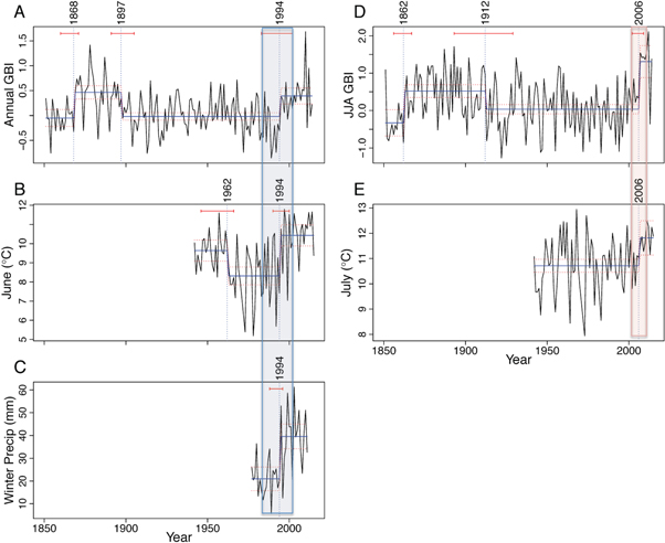
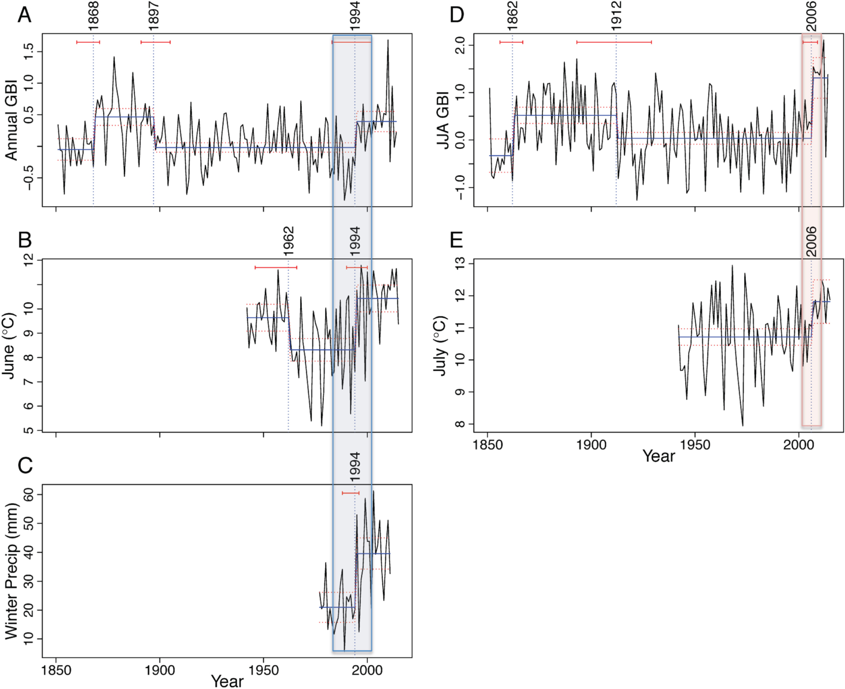
Figure 2. Nonlinear changes in the Greenland Blocking Index (GBI) and climate of the Kangerlussuaq region over time. Horizontal red bars depict significant breakpoints with 95% confidence intervals; when significant breakpoints were found, blue bars across data depict the average before and after breakpoints and red dashed lines show 95% confidence intervals around the fitted mean values of the response for periods between each break point.: (A) annual GBI with breakpoints (BPs) at 1868, 1897 and 1994; (B) mean June air temperatures from local weather stations, with BPs at 1962 and 1994; (C) winter precipitation (DJF) from local weather station, with BP at 1994; (D) summer (JJA) GBI with BPs at 1862, 1912, and 2006; and (E) mean July air temperatures from local weather stations, with BP at 2006. The period denoted as Winter/Spring BP indicated with blue box; period of Summer BP indicated by red box.
Download figure:
Standard image High-resolution imagePelagic limnological measurements
To evaluate shifts in physical and chemical lake water properties across the summer GBI breakpoint, pre- and post-2006 data were matched by lake and month of collection and log10 transformed. Pre-2006 lake water data were collected from 1998 to 2002; post-2006 were collected from 2013 to 15 (data and sample months provided in table S2). Conductivity and temperature were measured at a depth of 2 m using submersible probes. DOC concentration was analyzed in previous work (Saros et al 2015). Unfiltered total phosphorus (TP) samples were measured as soluble reactive phosphorus on a Lachat QuickChem 8500 following persulfate digestion. Secchi depth was used as a measure of water clarity, following the methods of (Saros et al 2016b).
Surface sediment diatom assemblages
The upper 0.5 cm of sediments from 18 lakes across the region were sampled for diatom analysis from the deepest part of the lake in 1998 and again in 2013. These surface sediment slices capture 1980–1998 and 1993–2013, respectively (ages determined by 210Pb dating). The earlier period primarily integrates time prior to and during the ∼1994 breakpoint, while the latter period captures all breakpoints plus post-breakpoint time. Samples were analyzed as described above. Diatom traits were determined following published procedures (McGowan et al 2018) and weighted averages of assemblages were calculated to summarize assemblage trait characteristics.
Statistical analyses
Piecewise linear breakpoints were used to identify significant fluctuations in the mean of each climate and environmental time series. Breakpoint analysis tests for the deviation from the null hypothesis of a simple linear regression model by minimizing the residual sum of squares through fitting subsets of the data to multiple regression coefficients. This method allows for multiple breaks and uses a Bai–Perron test (Bai and Perron 2003) to determine the optimal number of breaks using Bayesian information criterion (BIC, Schwarz 1978) and the residual sum of squares, given the minimum segment size of the time series (set at ∼5% of the observations). The location of these breakpoints can be attributed to the timing of non-linear changes in the observed environmental variable through time. Ninety-five percent confidence intervals were calculated for the observations associated with each breakpoint date (Bai and Perron 2003). All breakpoint analyses were conducted using the 'strucchange' package in the R Statistical Software (Zeileis et al 2002, R Core Team 2003), following published methodology (Zeileis et al 2003). For pre- and post breakpoint lake responses, differences between the two time frames were analyzed using paired t-tests.
Results and discussion
Time series analyses of regional climate systems (as GBI (Hanna et al 2016)) reveal few sudden changes in the atmospheric high-pressure region over Greenland until late in the 20th century. Using breakpoint analyses of the annual and seasonal GBIs spanning from 1851 to 2015, we document shifts during the period spanning from the end of the Little Ice Age into the early 20th century (figures 2(A), (D)). The next breakpoints do not occur until recent decades. Shifts to higher GBI values occurred in the annual series in 1994 (95% CI: 1988–2002; figure 2(A)) and in the summer series (JJA) in 2006 (95% CI: 2002–2009; figure 2(D)). Recent changes in the GBI are thought to relate to a more amplified northern polar jet stream owing to rapid surface warming in the Arctic, also known as the Arctic amplification (Francis and Vavrus 2015, Hanna et al 2016).
The climate of Kangerlussuaq shifted synchronously with the GBI (figure 2). Specifically, breakpoint analysis of mean monthly temperatures spanning 1942–2015 revealed shifts to higher values in June and July (figures 2(B), (E)); no other months were significant. Mean June temperatures shifted up 2.2 °C (from 8.3 to 10.5 °C) after 1994 (95% CI: 1991–2001; note an earlier breakpoint in 1962 indicated a decline from 9.6 °C to 8.3 °C). Mean July temperatures were more variable over the record prior to 1985, and rose 1.1 °C (from 10.7 °C to 11.8 °C) after 2006 (95% CI: 2004–2015). A winter (DJF) precipitation breakpoint at 1994 (95% CI: 1989–1997) indicated doubling of winter precipitation from 21 to 40 mm (figure 2(C)). Collectively, these results indicate two major shifts in West Greenland continental climate over the past 30 years: first, a shift to more snowfall and higher mean temperatures at the end of the spring thaw (June) since 1994 ± 6 years (hereafter referred to as the Winter/Spring Breakpoint (BP)), and later a shift to warmer conditions in summer (July, spanning 2004–2015; hereafter referred to as the Summer BP).
Nonlinear environmental responses occurred in coherence with these climate shifts (figure 3), suggesting strong extrinsic forcing of these responses. Lake ice out and terrestrial plant phenology are some of the ecosystem features most directly responsive to late winter and spring temperatures (Schindler et al 1990, Walther et al 2002); accordingly, they changed coherently with the Winter/Spring BP (figures 3(C), (E)). Modeled lake ice out shifted to 6 days earlier in 1993 (95% CI: 1979–2007; figure 3(C)). The modeled mean date of 50% plant species emergence advanced to 10 days earlier after 1992 (95% CI: 1989–1997; figures 3(E)). The Summer BP elicited an additional shift in plant phenology, with the modeled mean date of 50% plant species emergence shifting to 13 additional days earlier in 2009 (95% CI: 2008–2011). However, the plant phenology record represents community-averaged green-up dates, hence the first shift in phenology may be dominated by responses of early-season species, while the latter shift may be more dominated by the phenology of late-season species. A species-specific analysis in this region showed that early-season species underwent the most rapid advances in emergence timing, while late-season species showed slower or no advance at all (Post et al 2016). Later-season species may be more responsive to later season warming, in which case their phenology may be accelerated to a greater extent by summer warming compared to early-season species. We also note that in the case of the plant phenology response over time, both linear (R2 = 0.59, p < 0.001) and nonlinear (i.e. breakpoint analysis; R2 = 0.59, p < 0.001) goodness of fits were equal (table S1).

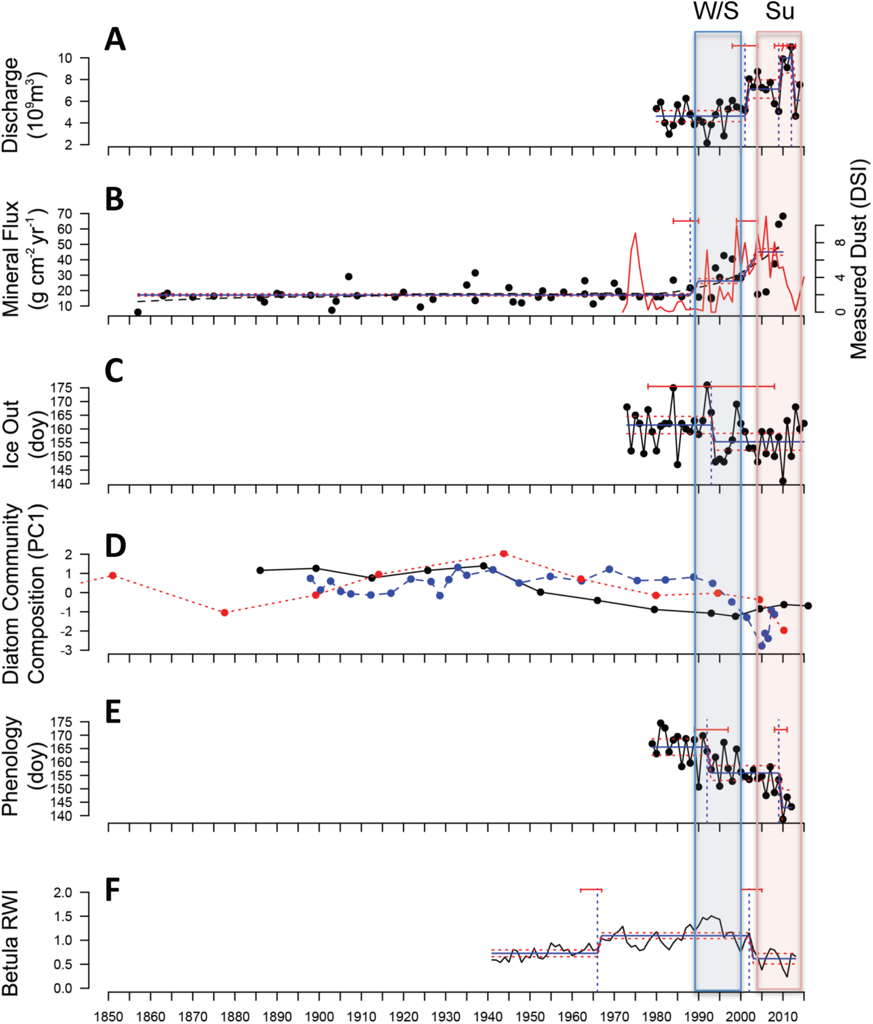
Figure 3. Environmental response across the Kangerlussuaq landscape over at least the past four decades. (A) Water discharge from the Greenland Ice Sheet; (B) dust (as mineral flux to lake sediments (black line) and as the instrumental Dust Storm Index (DSI; red line)) (C) day of year (DOY) of lake ice out; (D) diatom community turnover (as indicated by Principal Components (PC) Axis 1 scores, explaining 12%–21% of variance) in lake sediment records from SS901 (red), SS903 (blue), SS15 (black); (E) plant phenology (DOY of 50% species emergence across the entire local plant community); (F) shrub (Betula nana) stem Ring Width Index (RWI). Breakpoints are as defined in figure 2: period of Winter/Spring (W/S) Breakpoint indicated with blue box; period of Summer (Su) Breakpoint indicated by red box. Horizontal red bars above each response depict significant breakpoints with 95% confidence intervals; when significant breakpoints were found, blue bars across data depict the average for that period. Red dashed lines show 95% confidence intervals around the fitted mean values of the response for periods between each break point. Analysis of the dust record is only on the mineral flux record.
Download figure:
Standard image High-resolution imageOther nonlinear environmental responses occurred shortly after these climate shifts, with observed response lags consistent with internal system dynamics. Compared to 1979–2000, modeled GrIS discharge increased by 54% after 2001 (±3 years; figure 3(A)); the timing of this increase is coherent with a shift in observed discharge from nearby Tasersiaq catchment, where an abrupt 80% increase in discharge occurred in 2003 compared to 1976–2002 (Ahlstrøm et al 2017). This lag in response to the Winter/Spring BP may be expected as GrIS discharge responds to air temperatures, but during the first half of the year (which includes June), ice sheet snow cover further influences meltwater retention and retardation (van As et al 2017). Discharge rose another 40% in 2009 (95% CI: 2008–2011), overlapping with the Summer BP, although this additional increase was not sustained after 2012 (figure 3(A)). The mineral accumulation rate (min AR) of glacial outwash plain dust in lake sediment records increased by 53% in 1988 (95% CI: 1984–1990; figure 3(B)) compared to the period 1860–1988; this further increased 37% in 2000 (95% CI: 1999–2004).
The annual atmospheric DSI is shown for comparison to the min AR (figure 3(B)), and incorporates both the magnitude and frequency of observed dust events. Annual DSI was higher during 2000–2010 compared to 1973–2000 and driven by an increase in the number of severe dust events rather than the frequency of dust events. The second BP in the dust record (2000) coincides with the BP marking an increase in the GrIS discharge record. Sediment supply is primarily controlled by meltwater delivery from the ice sheet to the outwash plains although glacier dynamics may have contributed: since 2000, the glacier margin has thinned and areas with ice-cored moraines and debris-covered dead-ice have formed and increased the amount of debris available for deflation and enhanced dust events. Lake sediment records spanning from 1900 to 2014 showed the greatest changes in diatom community composition after 1990, however patterns varied across lakes (figure 3(D)). Change in diatom community composition gradually increased in lakes SS901 and SS15 from 1940 to 2000, accelerating in Lake SS901 during the Summer BP; in Lake SS903, it accelerated during the Winter/Spring and Summer BPs. These patterns underscore the multiple drivers, both external and internal to lake ecosystems, that determine diatom community responses, and consistently reveal that the greatest changes occurred after 1990. Based on shrub dendrochronology, Betula nana growth declined between the Winter/Spring and Summer BPs, with a shift to lower stem ring width index values by 0.11 in 2002 (95% CI: 2000–2005; figure 3(F)). Recent increases in herbivory with moth outbreaks and greater abundance of musk oxen are also considered important factors contributing to the decline in B. nana growth rate (Gamm et al 2018).
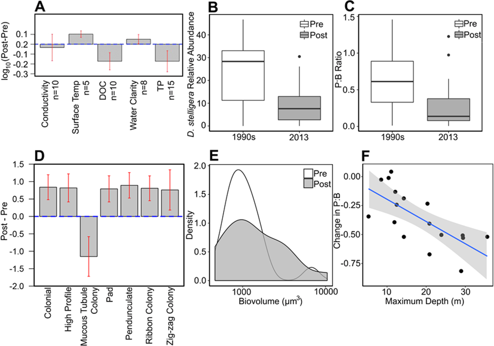
After the Summer BP, lakes became clearer and warmer during the open-water season (figure 4(A)). Comparing lake ecosystem features pre- and post-Summer BP, the temperatures of surface mixed layers increased, DOC concentrations declined and water clarity increased. Surface lakewater temperatures in this area are directly responsive to air temperatures (Kettle et al 2004). Declines in DOC increase water clarity and may be mediated by photooxidation (Cory et al 2014), which is amplified by earlier ice-out and prolonged light exposure. Lower DOC may also result from reductions in terrestrial subsidies to lakes (Anderson et al 2017), which can occur with warming-induced deepening of the soil active layer (Streigl et al 2005). Lakewater conductivity did not change over this period, indicating that declining DOC concentrations were not caused by dilution. Shifts in lake conditions altered habitat structure and rapidly led to major changes in primary producer communities. Earlier ice-out leads to deeper lake mixing depths in the summer (Olsen et al 2012). Pelagic diatom species responses are consistent with increased mixing depths: Discostella stelligera, an indicator taxon of shallower lake mixing depths (Saros et al 2016a), declined after the climate breakpoints (figure 4(B)). There was also a shift in diatom abundance from pelagic (P; open water) to benthic (B; lake bottom) habitats as indicated by a decline in the P:B diatom ratio (figure 4(C)). Functional traits of the diatom community diversified and became more complex after this BP, with increases in high profile (vertically elevated position in the biofilm) guilds including pad-attached, pedunculate (stalked) and ribbon/zig-zag colonial taxa (figure 4(D)) and a broader distribution of diatom cell size (biovolume) (figure 4(E)). These shifts suggest an expansion of the lake littoral zone into deeper waters leading to an increasing diversity of benthic habitats and complexity of diatom assemblages, indicating a broad change in ecosystem processes termed 'benthification' (Zhu et al 2006). Lake levels have changed heterogeneously across this landscape since 1995 (Law et al 2018). The mechanisms underlying the expansion of the littoral zone were therefore most likely initiated by the increases in water clarity, as well as lower average light exposure for plankton that results from deeper mixing depths (Olsen et al 2012). In agreement with this, P:B diatom ratios have changed the most in deeper lakes, which have a larger area available for littoral expansion and benthification (figure 4(F)). The increase in benthic taxa led to a positive feedback in which P recycled from sediments is sequestered by these taxa, reducing the amount available to phytoplankton (figure 4(A)) and reinforcing the clear water state (Genkai-Kato et al 2012). Increased dust inputs (figure 3) may further promote the benthic state, with dust sinking onto and fertilizing lake sediments (Shoenfelt et al 2017).

Figure 4. Lake response to the climate breakpoints. (A) Comparison of water column characteristics pre- and post-Summer BP, including dissolved organic carbon (DOC) and total phosphorus (TP), with number of lakes for each parameter indicated by n, red bars indicate 95% confidence intervals for the two-sided t-tests. Data for (B)–(F) are comparisons of fossil diatom assemblages in surface sediments of 18 lakes sampled in 1990s (integrate ∼1980–1998) and re-sampled in 2013 (integrate ∼1993–2013): (B) percent relative abundance of the indicator taxon Discostella stelligera, black bars represent the interquartile range of the data; (C) pelagic:benthic (P:B) of assemblages, with lower P:B suggesting greater proportion of benthic diatom taxa, black bars as in (B); (D) change in functional traits of diatom communities expressed as Post-Pre, red bars as in (A); (E) density plot of the distribution of diatom cell size (biovolume); and (F) change in P:B with lake depth, shaded area is 95% confidence region.
Download figure:
Standard image High-resolution imageConclusions
Numerous environmental features across this Arctic landscape were highly responsive to rapid climate change, revealing sensitive responses to abrupt extrinsic forcing of these ecosystems (figure 5). Two implications emerge from these results. First, nonlinear environmental responses driven here by extrinsic forcing were previously considered far less common than those arising from intrinsic nonlinear dynamics, often involving threshold-type responses driven in part by gradual change in drivers (Bestelmeyer et al 2011, Williams et al 2011). Some of the clearest examples from prior research came from paleoecological records spanning abrupt climate change events such as the transition from the Last Glacial Maximum (LGM)(Williams et al 2011) and the 8.2 ka cooling event (Tinner and Lotter 2001). Magnitudes of shifts in air temperature, atmospheric circulation and precipitation during the transition from the LGM were larger than those observed at present in Greenland, yet the nearly synchronous environmental response of this Greenland landscape to climate shifts in recent decades underscores the strength of climate forcing and the importance of the magnitude of these recent climate changes for ecosystem response. Second, tight coupling of environmental responses to climate shifts suggests strong, pervasive environmental changes in high latitude systems are expected with future abrupt climate change. Integrating this knowledge with tools that identify early warning signs of approaching threshold changes in the climate system (Lenton et al 2012) will better inform strategies to anticipate and manage future environmental response in the Arctic.
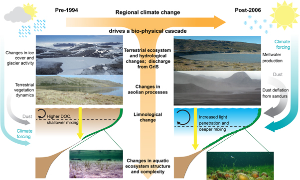
Figure 5. Conceptual model of the key components of the Kangerlussuaq landscape that have changed as a result of rapid regional climate change (indicated by the horizontal orange arrow and detailed in the main text). There are strong links among the key ecological and geomorphic systems (see Anderson et al 2017) which are illustrated by the four photographs: cryosphere changes, in the Greenland Ice Sheet (GrIS), snow cover and ice duration on lakes (upper left); changes in terrestrial vegetation and biogeochemistry (lower left); changing fluvio-glacial-hydrology indicated here by late-summer (August) meltwater discharge of the Watson River (upper right); changes in aeolian processes—intensity and frequency of dust storms (lower right). Subsequent shifts in ecological functioning and ecosystem structure in lakes indicated by the lake cross sections and the photographs of littoral zones of lakes. See main text for details of the process changes. Photograph credits: John Anderson, Jacob Clement Yde, Ole Pedersen.
Download figure:
Standard image High-resolution image
Acknowledgments
We thank Gordon Hamilton for assistance with satellite imagery, Johanna Cairns for figure rendering, and Peter Leavitt for constructive comments. Research funded by the US National Science Foundation (grant nos. 1203434, 1144423, 1525636, 1107381, and 0902125) and UK Natural Environmental Research Council (nos. NE/K000349/1 and NE/G019622/1) contributed to this work. This manuscript resulted from activities of the Kangerlussuaq International Research Network (KAIRN) at two workshops, funded by the Climate Change Institute of the University of Maine and by the Western Norway University of Applied Sciences.