

Abstract
Buildings and the atmosphere are intrinsically connected via cooling and heating systems. Global climate is projected to grow warmer, with an increasing fraction of the population living in urban centers. This introduces the challenge for new approaches to project future energy demand changes in cities. In New York City (NYC), the focus of our study, while air conditioning only accounts for 9% of all building energy end use, it is the main driver of annual peak electric demand. Here, we present end of century building cooling electric demand projections for NYC using a high resolution (1 km) configuration of the Weather Research and Forecasting model coupled to a building energy model and forced by bias-corrected CESM1 global simulations. High resolution urban canopy parameters such as building height and plant area fraction derived from a public tax-lot level dataset are used as input to the urban physics parameterization. Cooling demand increases in RCP4.5 ranged between 1% and 20% across all days, with largest increases on days below 50th percentile demand. Results show that end of century building cooling demand on days below the 50th percentile may be up to 80% higher than the 2006–2010 period in the RCP8.5 scenario. The largest percent increases per unit area were found over less densely populated boroughs of Brooklyn, Queens, and Staten Island. Maximum summer cooling demand for the entire city is projected to increase between 5% and 27% for RCP4.5 and RCP8.5, respectively. Overall, analysis shows a close to 8% increase in cooling demand per 1 °C increase in temperature.
Export citation and abstract BibTeX RIS

Original content from this work may be used under the terms of the Creative Commons Attribution 3.0 licence. Any further distribution of this work must maintain attribution to the author(s) and the title of the work, journal citation and DOI.
Introduction
Energy demand for building air conditioning is a considerable fraction of electric demand in the US. With temperatures in the Northeast US projected to increase throughout the 21st century (Hayhoe et al 2008), building energy demand and consumption are slated to also increase (Sailor 2001, Amato et al 2005). In New York City (NYC), summer air conditioning accounts for only 9% of annual energy consumption, yet it is the main driver of annual peak electric demand (NYISO 2017). Moreover, the New York Independent System Operator (NYISO) expects peak demand increases to outpace energy consumption change due to the larger need for space cooling under warming weather conditions. Additionally, cities are often warmer than their surrounding rural areas, a phenomenon called the Urban Heat Island (UHI), which may lead to larger cooling loads (Hsieh et al 2007, Santamouris 2014, Santamouris et al 2018). These UHI impacts on local temperatures have been shown to increase during extreme heat events (Li and Bou-Zeid 2013, Ramamurthy et al 2017, Ortiz et al 2018) due to positive feedbacks related to anthropogenic heat release and reduced urban soil evaporation.
Many studies of climate impacts on cities' energy demand have focused on statistical or physical process based methods to quantify building or total energy demand. In NYC, Howard et al (2012) modeled annual energy end-use by tax-lot with a multiple linear regression model, using building floor area and building function as the main predictors. Others have used neural networks to perform short term (24 h) forecasts at the utility-scale, obtaining errors of <5% in predicted peak loads (Park et al 1991). Beccali et al (2004) used an unsupervised neural network trained on multiple climatic variables to model suburban energy loads in Italy. Olivo et al (2017) quantified NYC energy consumption with a single building energy model (SBEM) applied to the city's entire building stock forced by weather data from the Typical Meteorological Year database. Ahmed et al (2017) followed a similar approach for Manhattan in NYC, forcing SBEM simulations with an actual weather forecast. They studied end-use energy demand and consumption based on 51 building archetypes for a single heat wave event.
A common approach involves using climate-derived indices such as cooling degree days (CDD) to relate climate impacts on cooling demand. This method has been used for Switzerland (Christenson et al 2006) to find potential increases in CDD between 13% and 17% across a multi-model ensemble. Cooling loads in tropical areas were derived from a multi-model ensemble (Angeles et al 2017) in low to medium emissions scenarios, finding mean total increases of over 8 GW for the Caribbean region. Lebassi et al (2010) used historical records to study CDD, demand, and consumption in California, finding large sensitivity to regional scale phenomena (e.g., increased sea-breeze impacting demand near the coast). Mukherjee and Nateghi (2017) found that mean dew point temperature was a better predictor of cooling and heating loads than CDD, with other climatic variables like wind speed and precipitation playing an important role.
A third method involves numerical weather prediction coupled with urban canopy models to study spatial-temporal variation of urban climate and cooling loads. This method has the advantage of accounting for feedbacks in the atmosphere-building envelope system, which might not be quantified with other techniques. In Japan, urban climate projections coupling the Weather Research and Forecasting (WRF) model to a single-layer urban canopy model across a multi-model ensemble (Kusaka et al 2012) found that heat stress hours were projected to increase by 62% by the 2070s. The single-layer urban canopy model was used to study cool roofs as a climate mitigation technology (Vahmani et al 2016) across RCP2.6 and RCP8.5 scenarios. This study found that cool roofs could offset city-scale climate-related temperature changes by up to 1 °C. Tewari et al (2017) studied combined impacts on cooling demand from climate change and urban expansion in the Phoenix and Tucson metropolitan areas using the WRF model coupled with a multi-layer urban canopy—building effect parameterization, (or BEP) and building energy models (BEM). They found that cooling demand per unit area may increase by up to 42.6% under the highest emissions scenario. Bueno et al (2011) coupled an SBEM to the town energy balance urban canopy model to quantify these impacts in Toulouse, France.
Quantification of energy demands at city scales has either focused on the use of statistical (Park et al 1991, Beccali et al 2004, Howard et al 2012) or process based (Ahmed et al 2017, Olivo et al 2017) models. One inherent limitation in these approaches is the lack of atmosphere-building envelope feedbacks that may take increased roles under a warming climate. An approach to resolve these impacts involves coupling numerical weather prediction to BEM (Bueno et al 2011, Kusaka et al 2012, Vahmani et al 2016, Tewari et al 2017). However, possibly due to computational cost and lack of detailed urban morphology data, studies have been limited to short time periods (<1 summer). Here, we present a study of end of century climate change impacts on summer cooling demand for NYC, using the WRF model coupled with a modified BEM across two emissions scenarios for a multi-year period.
Methods
Simulation setup
This study uses a high resolution configuration of the WRF model (Skamarock et al 2008) coupled with a modified multi-layer urban canopy and BEM parameterization as a tool to study changes in building cooling demand under climate change conditions. Regional-to-local scale projections are developed using bias-corrected runs of the Community Earth System Model version 1 (CESM1) (Brúyere et al 2015) dataset as initial and boundary conditions. Their work adjusts GCM by splitting data output into a seasonal signal and 6-hourly varying perturbation term representing the climate signal. The GCM's seasonally varying climatological signal is then substituted by its counterpart from ERA-Interim reanalysis between 1975 and 1994:

Here, CESMBC is the bias corrected CESM1, Obs is the reanalysis climatological mean, and CESM' is the CESM1 6-hourly perturbation term. Bias-correction of Global Circulation Models (GCMs) was shown to improve results of regional modeling forced with global models (Bruyère et al 2014). Sea surface temperatures from bias corrected CESM are updated daily. Specifically, temperatures over the continental US showed a decreased cold bias when all boundary condition variables were corrected with reanalysis data. Model physics used in this work follow the work of Gutiérrez et al (2015b) and Ortiz et al (2018) and are detailed in table 1. As the study concerns summer peak energy demand by end of century, only summers (1 June–31 August) were modeled, with a spin-up period of 3 days. Simulations are conducted for a historical (2006–2010) and end of century (2095–2099) periods. The domain extent (D01, figure 1) at a grid spacing of 9 km (119 points by 119 points) covers the Northeast Unites states and adjacent portions of the Atlantic Ocean. Domain resolution was increased via two-way nesting to 1 km (81 points by 84 points) horizontal grid spacing over the New York Metropolitan Area (D03, figure 1), with an intermediate 3 km (120 points by 120 points) resolution domain (D02, figure 1). The cumulus parameterization was turned off for the 1 km domain, as WRF can resolve convective processes explicitly at this resolution. There are 50 vertical levels, with 35 of them below 2 km height.
Table 1. Model physics parameterizations used in WRF simulations.
| Model physics | Parameterization |
|---|---|
| Land surface model | NOAH LSM (Tewari et al 2004) |
| Cumulus | Kain–Fritsch (Kain 2004), off in D03 |
| Microphysics | WSM6 (Hong and Lim 2006) |
| Urban canopy | Building effect parameterization (BEP) (Martilli et al 2002) |
| Building energy model (BEM) (Salamanca et al 2010) | |
| Cooling tower parameterization (Gutiérrez et al 2015a) | |
| Variable urban drag coeff. (Gutiérrez et al 2015c) | |
| Shortwave radiation | Dudhia (1989) |
| Longwave radiation | RRTM (Mlawer et al 1997) |
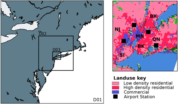
Figure 1. WRF simulation domains (left) and PLUTO-derived land use index inside D03. The boroughs of NYC are denoted shown: Brooklyn (BK), The Bronx (BX), Manhattan (MN), Queens (QN), and Staten Island (SI), as well as New Jersey (NJ) across the Hudson River.
Download figure:
Standard image High-resolution imageUrban canopy parameters are an important component in urban canopy models like BEP, providing urban morphology data necessary to compute energy and momentum exchanges with the atmosphere. Traditionally, these parameters have been estimated for different urban land use categories via use of look-up tables. Recent developments include disaggregation of urban land use classes from the commonly used 3-category classification (low/high density residential and commercial) to more a varied and descriptive scheme based on satellite imagery and a supervised classification algorithm, as in the WUDAPT project (Brousse et al 2016). A more costly approach involves measurements (often from aerial imagery) of urban canopy parameters at city-scales, as employed by NUDAPT (Ching et al 2009) for most major US cities. This work follows Gutiérrez et al (2015c), which employs a combination of tax-lot data with the existing NUDAPT database. High resolution urban canopy parameters, including building plant area fraction, height, surface to plant area ratio, and urban land use were derived from the NYC property land use tax-lot output (PLUTO), made available by the NYC Department of City Planning. PLUTO compiles building information at the tax-lot level, including floor area, number of floors, and facade width. Building parameters were interpolated into the D03 grid at 1 km spacing. PLUTO only provides information within NYC limits, so urban canopy parameters for grid points outside city limits were taken from NUDAPT. Figure 2 shows the 1 km resolution building area fraction and building height. PLUTO-derived parameters capture densely packed buildings in NYC, as well as the spatial heterogeneity of building heights, with expected maxima over downtown and midtown MN.
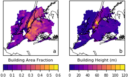
Figure 2. Building plant area fraction (a) and building height (b) parameters used in all simulations. Data is aggregated at 1 km grid spacing.
Download figure:
Standard image High-resolution imageWe consider two projection cases based on the representative concentration pathways (RCPs) (van Vuuren et al 2011): a stabilization scenario (RCP4.5) and a 'business as usual' scenario (RCP8.5). The RCP4.5 scenario projects increasing radiative forcing which stabilizes at 4.5 W m−2 by 2100, while RCP8.5 projects rising radiative forcing, reaching 8.5 W m−2 by end of century. Urban canopy parameters and land use classification in the projections are unchanged from the historical period.
Model evaluation
Model output is evaluated at the city-scale using load data from the NYISO. NYISO archives electric load at 5 min intervals for each of its load zones. NYISO divides New York State into 11 zones, with Load Zone J spanning the entirety of NYC. Load records can be found as far back as May 2001. Since NYISO only records the city's bulk load, and WRF only models building energy related to cooling and heating loads, a baseline load was computed based on Salamanca et al (2013). Baseline loads are calculated from the average of the day with minimum total load and the day with the lowest intra-day variability. For NYC, this typically occurs during May, when historical mean maximum temperature ranges between 19.4 °C and 23.8 °C (67–75 °F). This method has been used to successfully forecast total short-term (0–24 h) city-scale peak demand in NYC (Ortiz et al 2016). Simulated daily maximum temperatures and wind speeds are evaluated with station observations from four airports surrounding NYC (figure 1, right panel). For wind speeds, airport stations report any value < 1.5 m s−1 as calm conditions, so data points below this threshold in both WRF and CESM1 datasets are not considered. As peak demands occur on work days, all weekend and local holidays were removed from the dataset.
Results
Electric load and near-surface climatic variable evaluation
Historical period simulations are evaluated against both bulk city-scale daily peak load data from the NYISO and airport station temperature observations (figure 3). Simulated results are compared against kernel density estimates (KDE), an approximation of a dataset's distribution. One advantage of KDE is that they do not require bins to group data samples. Results show WRF total mean daily peak demand of 9220.8 MW (figure 3(a)), overestimating mean daily peak demand from NYISO of 8962 MW, or by 2%. Model standard deviation (429 MW), however, underestimates observations' value (1070.2 MW) by 59%. NYISO recorded a maximum load of 11 305.5 MW, while the WRF maximum was 9569.6 MW, an underestimation of about 15%. Model performance is partly explained by lack of inclusion of non-building loads such as the NYC subway system and street lighting, which a constant baseline may not account for. For example, NYC Transit, including buildings and subway infrastructure, averages 200 MW electric load, growing to 350 MW during peak hours, with an additional 96 MW added from newly constructed subway lines (Metropolitan Transit Authority 2003). Other potential causes are failure to accurately capture building occupancy in simulations, which are assigned a simplified daily schedule in BEM for each urban class.

Figure 3. Kernel density estimates of (a) daily peak load, (b) 2 m temperature, and (c) 10 m wind speed for the historical simulation period from observations and WRF simulations. Meteorological variables also include bias corrected CESM1 (BC-CESM1) used as initial and boundary conditions.
Download figure:
Standard image High-resolution imageModel evaluation against weather station data shows that WRF simulated daily maximum temperature improves on the input CESM1 data in both model mean and standard deviation (figure 3(b)). Airport stations reported a mean daily maximum of 28.41 °C with a standard deviation of 3.69 °C. WRF simulations results, interpolated using nearest neighbor showed a mean daily maximum of 28.66 °C (0.88% error) with a 3.37 °C standard deviation (9.5% error), whereas BC-CESM1 showed a 26.54 °C mean (6.6% error) and 2.87 °C standard deviation (14.8% error). These results are consistent with Bruyère et al (2014), which found reduced cold biases in near surface temperature distributions when forcing WRF with bias-corrected climate data. Winds are, in general, underestimated in the WRF simulations for values below 5 m s−1, by nearly 0.5 m s−1, while overestimating occurrence of winds over 6.5 m s−1. While BC-CESM1 follows the shape of the observations' distribution, it does not capture high wind values (>10 m s−1), at all whereas WRF simulations reach values of 18 m s−1, where observations report a maximum of 21.9 m s−1.
Cooling load projections
Peak cooling demand projections are presented as percent (%) increases over 2006–2010 across different points in the distribution of cooling demand (figure 4). In RCP4.5 (figure 4(a)), cooling demand increase ranges from 1% to 20% across all values. Throughout the city, percent increases are larger in BK, QN, and SI. Manhattan, dominated by taller, more densely packed buildings, accounts for the highest absolute 2006–2010 cooling load per unit area (table 2), leading to lower percent increases. Cooling demand increases are highest, in general, at the 25th percentile, over QN and SI, reaching up to 18%. Demand increases are lower overall on days above 75th and 90th percentiles demand (figure 4, third and fourth panels), which average 11.13% and 10.73%, respectively, over the historical period, whereas the 25th and 50th average 9.1% and 8.9%, respectively. Maximum summer peak demand is an important metric for utilities, as it is indispensable for planning of generation and transmission resources. Maximum peak cooling demand for the projection period was 3016.7 MW, representing an increase of 5.4% over the simulated 2006–2010 value.
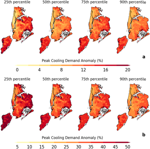
Figure 4. Peak air conditioning demand increase from 2006 to 2010 for 2095 to 2099 under (a) RCP4.5 and (b) RCP8.5.
Download figure:
Standard image High-resolution imageTable 2. Median building peak AC energy demand per building unit area (W m−2) for the historical and two projection scenarios (2095–2099). Values in parenthesis show percent increase over historical period. BHGT indicates mean building height in each borough.
| 2006–2010 | RCP4.5 | RCP8.5 | BHGT | |
|---|---|---|---|---|
| Bronx | 57.3 | 62.8 (9.9%) | 75.0 (31.7%) | 16.0 |
| Brooklyn | 42.9 | 46.8 (9.4%) | 56.15 (31.2%) | 13.8 |
| Manhattan | 81.1 | 86.5.5 (6.8%) | 102.1 (26.4%) | 47.7 |
| Queens | 42.9 | 47.3 (10.5%) | 57.9 (35.5%) | 11.0 |
| Staten Island | 42.11 | 46.9 (14.4%) | 58.3 (41.9%) | 9.2 |
In RCP8.5 (figure 4(b)), cooling demand increases are much larger than RCP4.5, reaching past 80% compared to 2006–2010. The largest changes are observed at the 25th (38% increase) and 50th (35% increase) percentiles, a reversal of the trend observed in RCP4.5. On the warmest days (figure 4(b), 90th percentile), percentage increases are not as large due to large historical period cooling demand, under 25% over MN and 35% over BK and QN. Increases are largest over relatively suburban SI, between 35% and 45%. Similar to RCP4.5, the largest cooling load anomaly occurs in the cooler half of all summer days, when percent changes reach up to 80%. Similarly to RCP4.5 projections, largest increases occur over BK, QN, and SI, and growing lower with distance to the southeastern shore. This scenario produces a significantly larger maximum total cooling demand of 3644.4 MW, a 27.3% increase over the historical period.
Temperature and cooling load
Simulated peak demand increases per NYC borough as summarized table 2 show spatial heterogeneity. This is due both to the geographical heterogeneity of the urban canopy across the city (figure 2) as well as spatial variability in climate projections. Larger baseline loads in the 2006–2010 period in areas with taller buildings (e.g., Manhattan), experience larger unit load increases, but lower percent increases in end of century scenarios. Although building stock characteristics are kept constant in all simulations, temperature changes are not. Defining a historical climatology for each grid point as the mean 16:00 LST temperature and cooling demand (T2hist and AChist), end of century anomalies were computed as

Here, T216lst,2095–2099 and AC16lst,2095–2099 represents temperatures and cooling loads at 16:00 LST for every grid point in D03. Results show a strong (figures 5(a) and (b)), almost linear relationship between T2anomaly and ACanomaly in both RCP4.5 and RCP8.5. For 4.5, a linear regression shows an increase of 8.1% cooling demand per 1 °C increase in temperature with a coefficient of determination (R2) of 0.89, and p-value < .001. For RCP8.5, a similar relationship was found, with an increase of 7.7% cooling demand per °C increase in temperature, coefficient of determination (R2) of 0.86, and p-value < .001. RCP8.5 results show more spread, with a standard error in the regression of 19.74 × 10⁻⁴, whereas regression for RCP4.5 has a value of 21.82, a 10.5% difference. RCP8.5 exhibiting more spread suggests a more variable climate, which may lead to challenges in building demand prediction and management.

Figure 5. Hex bin plot of percent increase per grid point AC demand as a function of near surface temperature (a), (b) and heat index (c), (d) anomalies for RCP4.5 and RCP8.5. Color map represents count number per hexagonal bin. Bins with counts < 100 have been omitted.
Download figure:
Standard image High-resolution image
Other possible predictors of cooling demand change may include a measure of air moisture content, an important component in air conditioning systems. One such estimator is the heat index (Rothfusz 1990), which combines relative humidity and temperature to measure temperature experienced by humans in shaded areas. AC demand increases anomaly was compared to simulated heat index anomaly (figures 5(c) and (d)). Results indicate that although a strong correlation exists with heat index, with coefficients of determination of 0.83 and 0.79 for RCP4.5 and RCP8.5, respectively, it is not as good an estimator of ACanomaly as 2 m air temperature. Additionally, ACanomaly is less sensitive to changes in heat index, showing increases of 6.5% and 5.8% per 1 °C in heat index for RCP4.5 and RCP8.5, respectively.
Conclusions and future work
In this study, a high resolution urbanized configuration of the WRF model was used to project building cooling demand for the city of New York by end of century. Two scenarios were explored, RCP4.5 and RCP8.5, representing stabilization and high emissions scenarios, respectively. As seen in the results section, changes in daily peak cooling demand shows strong geospatial heterogeneity across NYC. In general, locations closer to the southern coast (BK, QN, SI) show largest variability across cool and warm days. Largest increases are observed in days below the 50th percentile of cooling demand, more evident in the high emissions scenario, suggesting a decrease of cool summer days. Meanwhile, end of century summer maximum demand for cooling could increase by 5% in RCP4.5, and around 27% in RCP8.5 on average. Percent increases per unit area were found to be more sensitive to changes in temperature rather than heat index, with sensitivity ranging between 7.7% and 8.1% AC demand increase per 1 °C daily maximum temperature increase. This sensitivity is particularly important, as simulated maximum temperature anomaly could reach over 15 °C, leading to more than a doubling in peak demand on particular days.
One limitation of this impact study is the assumption that 100% of indoor spaces are cooled. This limiting assumption is due both to lack of information on air conditioning system adoption at the city scale as well as current technical limitations of the BEM parameterization. Many cities have begun to mandate benchmarking of energy use for certain buildings. NYC specifically, requires buildings with floor area of at least 500 00 (47% of all buildings) to report on energy use across several categories (e.g., hot water, cooling, heating), which may lead to better understanding of air conditioning adoption and trends (Local Law 84 of 2009). Recent work has addressed the latter limitation by introducing a cooled fraction parameter into BEM which can be assigned on a per grid point basis (Xu et al 2018). Moreover, this study only considers impacts of climate on NYC's current building stock. Potential urban expansion and re-development within the city may strengthen urban-atmosphere feedbacks (Georgescu et al 2012), while adaptation-focused policies (e.g., cool roofs/areas, AC efficiency measures) can potentially reduce them. For example, programs like the US Department of Energy Energy Star, incentivize building and equipment energy efficiency and may help offset some of the climate impacts on cooling loads. However, studies have shown that warmer conditions in urban neighborhoods may decrease air conditioning COP by over 15% (Gracik et al 2015), which might be exacerbated under increasingly warm summers. Finally, future work may expand simulations via use of an ensemble of GCM runs, which would allow for an estimation of uncertainty in projections of climate impacts.
Acknowledgments
The work presented here has been made possible through the NOAA-CREST Grant NA17AE1625. Computational resources were provided by the CUNY High Performance Computing Center, funded in part by grants from the City of New York, New York State, CUNY Research Foundation, and National Science Foundation Grants CNS-0958379, CNS-0855217, and ACI-1126113.