


Abstract
In the western United States, 27% of electricity demand is met by hydropower, so power system planners have a key interest in predicting hydropower availability under changing climate conditions. Large-scale projections of hydropower generation are often simplified based on regression relationships with runoff and they are not always ready to inform power system models due to the coarse time scale (annual) or limited number of represented power plants. We developed an enhanced process-based hydropower model to predict future hydropower generation by addressing the commonly under-represented constraints, including (1) the ecological spills, (2) penstock constraints to provide flexibility in electricity operations, and (3) biases in hydro-meteorological simulations. We evaluated the model over the western United States under two emission scenarios (RCP4.5 and RCP8.5) and ten downscaled global circulation models. At the annual time scale, potential hydropower generation is not projected to change substantially, except in California. At the seasonal time scale, systematic shifting of the generation patterns can be observed in snowmelt-dominated regions. These projected annual and regional trends are comparable to other regression-based relationships. However, the representation of more complex operations and constraints tend to reduce the uncertainties inherent to climate projections at seasonal scale. In the Pacific Northwest region where hydropower is the dominant electricity source, our predicted future change of hydropower generation is about 10% less than the regression-based projections in spring and summer. The model can also capture the seasonal non-stationary in hydrologic changes. The spatio and temporal scales of the model, increased accuracy and quantification of uncertainty allow one to use the products to inform power system models toward supporting energy sector planning activities and water-energy trade-offs.
Export citation and abstract BibTeX RIS
1. Introduction
Hydropower is a clean, affordable, and renewable energy source that has served the United States (US) for more than a century (US Department of Energy 2016). In the western United States, where the gross potential is relatively large due to the mountainous terrain, hydropower holds a significant role in the energy portfolio; it accounts for about 27% of total electricity generation (WECC 2017). Unlike fossil fuel power, the 'fuel' of hydropower is available river discharge that could enter the dam turbine, and discharge is sensitive to upstream hydrometeorological conditions. Previous research has shown that the spatiotemporal patterns of water resources are expected to shift under conditions of climate change, especially in snow-dominated regions because of the near-surface warming caused by increased greenhouse gas emissions (Barnett et al 2005, Hamlet et al 2010, Van Rheenen et al 2004). The non-stationarity of water resources availability induced by climate change will directly affect potential future hydropower production (Hamududu and Killingtveit 2012, Kao et al 2015, van Vliet et al 2016, Turner et al 2017).
There are two types of approaches that have been typically used to predict future hydropower generations. Regression-based approaches are based on linear regression relationships between observed historical natural runoff and hydropower generation (e.g. Kao et al 2015, Bartos and Chester 2015, Voisin et al 2016), with the advantages of being simple, providing projections that agree very well with observed historical means and representing historical inter-annual variability. The challenges with this approach however are that it fails to capture non-linearity in power generation response to changes in hydrology among other changes: the underlying assumptions of the linear regression are that constraints on operations are static (environmental, flood control, water supply, and spinning reserve versus generation operations) and that the reservoir storage can buffer the potential changes in hydrologic regimes.
In contrast, process-based hydropower projections are based on the regulated runoff with explicit daily to monthly reservoir storage simulations. These projections usually are informed by the same physically based hydrologic simulations as regression-based approaches, and they provide estimates of potential hydropower (actual generation and spinning reserve, i.e. if turbine flow rate is at its maximum capacity constantly). Hydropower generation (P, in MW) is usually computed using the following equation:
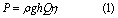
where ρ is the water density (1000 kg m−3), g is gravitational acceleration (9.81 m s−2), h is the hydraulic head of the dam (m), Q is the turbine flow rate (m3 s−1), and η is a non-dimensional efficiency term. This approach has been adopted in many large-scale energy assessment studies based on regulated or even natural runoffs (e.g. Lehner et al 2005, van Vliet et al 2013, 2016, Liu et al 2016, Turner et al 2017). This simple process-based model provides the total potential hydropower generation that could be used for both reserve and generation services to the electric grid. Hydropower is often not used with full turbine flow rate capacity in order to provide flexibility to electricity grid operations and allow for quick changes in electricity demand as well as contingency generation if a power plant in the system was to stop generating unexpectedly. This flexibility is referred to here as 'reserve'. By incorporating reservoir storage variations, the model can capture non-stationarity in power response to hydrologic regime shifts, which affect both streamflow and reservoir head levels. However, these approaches could be improved further with power plant fleet details (multi-reservoir systems), unbiased hydro-meteorological input data, and an expanded set of operating constraints (Fernandez et al 2013, van Vliet et al 2013, Kao et al 2015). Among the set of constraints, we note two here:
- Hydropower operations provide multiple services to the grid, including generation and reserve. According to the western electricity coordinating council's (WECC's) contingency reserve guidance (NERC 2015), the reserve should be the greater value between (1) power loss from single most severe contingency, or (2) 3% of load plus 3% of generation. Additionally, half of the reserve should be fulfilled as spinning reserve, which means no power will be generated. Without the representation of spinning reserve, projections of hydropower actual generation are most likely overestimated.
- Another constraint on hydropower generation operations is the mandatory ecological spill, which provides salmon access to their natural spawning and rearing habitats in river basins along the Pacific Coast (Leonard et al 2015). The Bonneville Power Administration, a federal power marketing agency based in the Pacific Northwest, reported an about $2.88 billion USD revenue loss from 1978–2012 related to aiding dam passage of juvenile and adult anadromous fish via water spilling (NPCC 2013).
In this study, we enhance the process-based hydropower modeling approach by explicitly representing these generation constraints in addition to addressing integrated hydro-meteorological simulations biases. The predictions of this model are consistent with power system model forcing requirements such as PROMOD4 and PLEXOS5 across spatial and temporal scales (all hydropower plants and daily time steps, with calibration at a monthly time scale), which can be directly used for holistic long term electricity grid operations planning. Table 1 summarizes existing approaches that also estimate hydropower generation, with associated assumptions and resolution used by a number of large scale studies. Table 1 also highlights the enhancements of this approach.
We combined the model with a two-step multiscale calibration approach first to address the errors in annual hydro-meteorological biases at the scale of hydrologic regions, and second to reflect the complexity in monthly multi-objective reservoir operations and daily generation constraints, such as penstock intake capacity, dynamic power grid reserve requirement to not use penstock at full capacity, and dynamic ecological spills at the scale of energy regions.
Table 1. Hydropower model used in this study compared with other commonly used models.
| Study | Method | Estimate | Simulated period | Spatial scale | Flow regulation | Storage head | Ecological spill | Grid reserve margin service | Power-plant-level estimates |
|---|---|---|---|---|---|---|---|---|---|
| Lehner et al 2005 | Simple process-based | Potential hydropower for every grid cell | 1 scenario, 2 GCMs | Europe, half deg | No | Fixed, based on DEM | No | No | No |
| van Vliet et al 2013 | Simple process-based | Potential hydropower for every grid cell | 2 scenarios, 6 GCMs | Europe, half deg | No | Fixed, based on DEM | No | No | No |
| Kao et al 2015 | Regression-based | Hydropower generation at plant level | 1 scenario, 1 GCM | Four regions across the US, 1/8th deg | No | N/A | No | No | Yes |
| Bartos and Chester 2015 | Regression-based | Hydropower generation at plant level | 3 scenarios, 2 GCMs | Western US, 1/8th deg | No | Fixed based on the dataset | No | No | Yes |
| van Vliet et al 2016 | Simple process-based | Potential hydropower at plant level | 2 scenarios, 5 GCMs | Global, half deg | River routing—water management model | Varies, simulated by water management model | No | No | No |
| Voisin et al 2016 | Regression-based (rescaling) | Hydropower generation at plant level | Historical | Western US, 1/8th deg | Observed monthly regulation rescaled based on simulated regulated flow deviations | N/A | No | No | Yes |
| Turner et al 2017 | Simple process-based | Hydropower generation at plant level | 2 scenarios, 3 GCMs | Global, half deg | Reservoir optimization model , no river routing | Varies, simulated by reservoir optimization model | No | No | Yes |
| This study | Enhanced process-based | Hydropower generation at plant level | 2 scenarios, 10 GCMs | Western US, 1/8th deg | River routing and water management model | Varies, simulated by water management model | Yes | Yes | Yes |
Using the enhanced hydropower model, we project hydropower estimates under future climate conditions over the western US. We systematically evaluate the contribution of calibration with respect to observed generations at two spatial scales: balancing authority (BA) scale and reserve energy region scale in order to provide an evaluation at scales that have direct impacts on power system dynamics. The BA scale is equivalent to province or country scales for economics and long term planning decision making, while the reserve energy region scale is an aggregation of BAs usually for systematic security assessment and monitoring.
The objective of this paper is to advance on the assessment of climate change impact on hydropower generation at scales and accuracy levels relevant to long term power system planning and policy-making (Tidwell et al 2016, 2018). The new modeling framework and analytics, which combine hydrological and energy scales and represent hydropower generation constraints, aim to provide a systematic approach to improving the understanding of the dynamics of co-evolving water and energy systems.
2. Method
2.1. Study area and data
Our study area covers the US part of the Western Interconnection (power grid), which is managed by the WECC (figure 1). The area encompasses five main hydrologic regions (Pacific Northwest, California, Great Basin, Upper and Lower Colorado River Basin) and headwaters of three other large regions (Missouri, Rio Grande, Arkansas-Red). The WECC domain can also be disaggregated into 36 BAs (excluding the two in Canada and one in Mexico), which correspond to the energy regions explicitly represented in power system models. In each BA, the energy demand must be balanced at all times first by local generation sources and then by external resources through the transmission system.

Figure 1. Study region with color-coded reserve regions across the WECC.
Download figure:
Standard image High-resolution imageThe BA regions in the study area have a combined nameplate capacity of about 55 400 MW contributed by more than 500 hydropower plants (WECC 2017). The database that includes the location, nameplate capacity, and BA dependency of the hydropower plants were extracted from the WECC TEPPC (Transmission Expansion Planning Policy Committee) 2024 common case and using infrastructure present in 20106. The database is used to set up commercial production cost models such as PLEXOS and PROMOD among others, and are widely used over the WECC (Ibanez et al 2014, Voisin et al 2018) to model the unit commitment and dispatch of generators to minimize the production cost of the power grid system. In this study, we simulated the flow regulation based on over 500 reservoirs operated for a range of purposes (water supply, flood control, etc) (Voisin et al 2017, Zhou et al 2018) and we explicitly simulate hydropower at the 149 individual hydropower plants that had a capacity greater than 50 MW, collectively accounting for about 51 000 MW or 92% of the total capacity across the WECC. These simulated power plants are located in 24 out of 36 BAs in the study area. The geometric information for the simulated power plants, such as the dam height and volume capacity of the associated reservoirs, were taken from the Global Reservoir and Dam database (Lehner et al 2011) or the National Inventory of Dam database (whichever was applicable).
Reserve regions represent another energy scale. They consist of aggregations of BAs, within which a reserve margin needs to be maintained (NERC requirement). We considered five reserve regions (i.e. the Northwest, California, Great Basin, Desert-Southwest, and Rockies) (WECC 2013). In our study, we developed a hydropower model with projections calibrated for BAs which include large simulated hydropower plants (total of 24). However, for simplicity, the analysis was performed at the scale of the five reserve regions (figure 1). The BA scale analysis can be found in the supplemental material.
2.2. Future climate and runoff projections
Future hydro-meteorological conditions and associated uncertainties were represented by 10 General Circulation Models (GCMs; CCSM4, GFDL-CM3, GFDL-ESM2M, INM-CM4, MIROC5, MIROC-ESM-CHEM, ACCESS1.0, HadGEM2-CC, HadGEM2-AO, and NorESM1-M) selected from the Coupled Model Intercomparison Project Phase 5 (CMIP5) (Taylor et al 2012). The selected models span a range of temperature and precipitation projections for the study region (figure S1 and S2 in supplemental material available at stacks.iop.org/ERL/13/074035/mmedia). We chose the representative concentration pathway (RCP) scenario in which anthropogenic radiative forcing reaches 8.5 Wm−2 by the end of the 21st century (RCP 8.5) (Moss et al 2010) to represent the most extreme scenario in terms of global greenhouse gas emissions with minimal efforts being placed on energy demand controls (Riahi et al 2011) and RCP 4.5 as a low scenario in which greenhouse gas emissions stabilize by mid-century and fall sharply thereafter (results of RCP 4.5 scenario are presented in the supplemental material). The ten GCM-projected precipitation and temperature data sets were first statistically downscaled and bias-corrected to 1/8th degree resolution relative to the observed (1950–1999) climate using a Bias Correction and Spatially Disaggregation approach (Wood et al 2004). Then, the Variable Infiltration Capacity model (Liang and Lettenmaier 1994) was forced to simulate the projected daily runoff fields across the western US at 1/8th degree resolution. These data were made available online by the Bureau of Reclamation (ftp://gdo-dcp.ucllnl.org/pub/dcp/archive/cmip5/hydro/). Readers are referred to Wood and Mizukami (2014) for details about this runoff data set.
2.3. Water management model and hydropower production model
The gridded runoff fields were then used to force a large-scale water management (WM) model (Voisin et al 2013a), coupled with a plant-level, enhanced process-based hydropower generation model (figure 2) for future hydropower predictions. The water management model consists of a grid-based river routing model: the Model for Scale Adaptive River Transport (MOSART; Li et al 2013), and a water management component, which was used to simulate future regulated river flow. The operating rules of the reservoirs are a set of monthly release and storage variations patterns that are associated with meeting primary water uses, i.e. flood control, or irrigation, or combined flow control and irrigation. The releases of reservoirs follow the operating rules and are further determined at seasonal, monthly and daily time scales based on water year conditions (wet, dry), reservoir storage characteristics (minimum and maximum storage), water demand associated with the reservoirs and other release constraints (minimum environmental flow release). Details about how the operation rules are determined can be found in Voisin et al (2013a). The WM model has been shown to represent seasonal variations in regulated river flows across the US (Voisin et al 2013a, 2013b, Hejazi et al 2015, Voisin et al 2017, Zhou et al 2018) and is similar to other large-scale water management applications in terms of handling water withdrawal and dam operations (Hanasaki et al 2006, Biemans et al 2011, van Vliet et al 2012, Döll et al 2012, Zhou et al 2016).
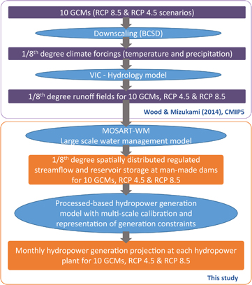
Figure 2. Model coupling scheme.
Download figure:
Standard image High-resolution imageThe WM model was forced by the Reclamation-projected runoff fields at 1/8th degree resolution in nine Hydrologic Unit Code 2 regions that cover our study area. The model simulated 950 reservoirs (yellow triangles in figure 1) with basic information (functionality, storage capacity) taken from the GRanD database and provide storage variations and release for the 950 reservoirs. Only 149 of those 950 are powered dams and the hydropower model leverages the MOSART-WM simulated storage variations and releases at those 149 reservoirs only. The gridded water demand was derived from the integrated Global Change Assessment Model (Hejazi et al 2015), which considers multiple water demand sectors and a number of socioeconomic variables such as population, labor productivity, and technology (Edmonds and Reilly 1985, Edmonds et al 1997, Kim et al 2006). We used the water demand at a fixed 2010 level, which had been calibrated and evaluated (Voisin et al 2013b, Hejazi et al 2015) with respect to the demands reported by the US Geological Survey (Kenny et al 2009). The MOSART-WM model was run at daily time steps from 1981–2095 after a 5 year spin-up period. The regulated flow rates at the 149 simulated hydropower plants (capacity >50 MW) were extracted as input for the process-based hydropower generation model. For power plants associated with reservoirs, the WM model-simulated storage time series were also extracted for the power model to derive the hydraulic heads.
The enhanced process-based hydropower generation model (figure 3) first determines whether the simulated power plant is associated with a reservoir. In the simulated 149 hydropower plants, 74 of them are Run of River (ROR) dams for which reservoir storage variations are not explicitly simulated, and only the flow is used to estimate generation. For ROR plants, the hydraulic heads (h, m) were assumed to be unchanged and equal to the dam height (H, m). For plants associated with reservoirs, the hydraulic heads at each time step were estimated based on the WM model-simulated storage (V, m3) time series by assuming the shape of the reservoir is a tetrahedron (Fekete et al 2010) as represented by
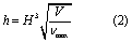
where Vmax is the volumetric capacity (m3) of the reservoir.
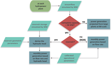
Figure 3. Flowchart of the enhanced process-based hydropower generation model developed in this study.
Download figure:
Standard image High-resolution imageAfter the hydraulic head was determined, a number of parameters were introduced into the power model to adjust the runoff and to constrain the generation at each simulated power plant. The parameter set included (1) a bias correction factor (fb, ranging from 0.5–1.5), which accounts for the bias of annual runoff and generator efficiencies; (2) 12 monthly spill correction factors (fs1, fs 2, ..., fs12, ranging from 0.5–1.5), which determine the mandatory spills for ecological purposes and spinning reserve; and (3) a penstock intake adjustment factor (fp, ranging from 0.5–1.5), which determines the actual maximum intake of the penstock relative to the reported penstock capacity. All 14 parameters were calibrated in a two-step multiscale calibration process (see details in section 2.4) and further applied to estimate the future hydropower generations in the 21st century under the RCP 4.5 and RCP 8.5 scenarios.
2.4. Power model calibration
We developed a two-step multiscale calibration process to meet the forcing requirements of power system models. The observation data used in the calibration were the monthly actual power generation totals for the 149 large hydropower plants reported by the US Energy Information Administration (EIA; available at www.eia.gov/electricity/data/eia923/). The target parameter of the first step was bf, which addresses overall bias in hydro-meteorological model simulations including WM and water demands at an annual time scale. The model was calibrated against the annual potential generation (PG, in MW), equivalent to the actual generation (G, in MW), plus the operating reserve (R) at the BA region scale. The R was assumed to be fixed at 4% of the total load (TL) of each BA region to be consistent with typical power system model applications (Schlag et al 2015). The TL was assumed to be fixed at the 2010 level throughout the calibration period (2001–2014). In a BA region with n hydropower plants, the fb was calibrated using the shuffled complex evolution (SCE) auto-calibration algorithm (Duan et al 1993) to minimize the mean absolute error between annual the time series of PGBA_sim and PGBA_obs, where

and

in which TL2010 was obtained from PLEXOS database and Gobs was the actual annual power generation from the EIA. In this step, the hydropower generation of the BA region was represented by aggregating only the large hydropower plants (>50 MW).
The second step aimed at improving the seasonal variation for each power plant by calibrating fs and fp. In this step, the fb calibrated in the previous step was set to be fixed for each plant. At each power plant, the SCE algorithm was again applied to reduce the Kling-Gupta Efficiency (Gupta et al 2009) between the simulated monthly power generation time series (Gsim) and Gobs over the calibration period with

where fs,m is the spill correction factor at m month, S is the turbine nameplate capacity, and S × fp reflects the maximum intake capacity of the penstock.
Given that the observed hydropower generation (from the EIA) is relatively short (14 years), we calibrated the model against the entire record and evaluated the model using the leave-one-(year)-out cross-validation (LOOCV) technique to determine whether the model was over-fitted. LOOCV is a repeating cross-validation process that uses each single-year observation as the validation data and the remaining 13 years of observation to build the model. The statistics evaluated using LOOCV for each validating year were also compared with the predictions from the final model (based on 14 years). The calibration results are presented in the following section.
3. Results
3.1. Model calibration results
We first evaluated the two calibration steps by comparing the observation with predicted hydropower generations before and after each step of calibration. The 'before calibration' setup is a physically based estimate that assumes all calibrated parameters are equal to 1, meaning there were no corrections to annual hydrology, no ecological and reserve spills on monthly runoff, and no adjustment of the maximum nameplate capacity. The 'after 1st calibration step' represents the potential hydropower generation estimates with realistic annual hydropower generation, but does not represent any constraints on monthly generation. The 'after 2nd calibration step' is the final product to be evaluated and includes monthly constraints. The comparisons were conducted at the seasonal scale (see figure S3) and with statistical metrics (mean absolute relative error and correlation coefficient) for all reserve regions summarized in figure 4. The results suggested that generation based on unbiased corrected integrated water modeling could lead to a large annual bias, while the two-step calibration substantially decreased the bias and improved the seasonality of the predictions. In the following analysis, we refer to the 1st step calibration estimate as 'a regression-based estimate' to represent studies based on regression analyses with observed hydropower generation, and evaluate the difference in projections when complex monthly generation constraints are represented.
Second, we checked the LOOCV results and compared them with the final model predictions at each validated year across the predicted BA regions (figure S4). The LOOCV results revealed that in 11 out of 14 years the median relative absolute error was less than 0.2, and in all years except 2001 the monthly correlation coefficients were over 0.6. This result suggests that the model was not over-fitted and the model parameters represent the physical processes of the hydropower generation. The statistics between the LOOCV models and the final model were similar, indicating that the overall prediction skill of the final model can be represented by the LOOCV models.
3.2. Projection of future hydropower generation
By applying the calibrated hydropower model to the WM model's simulated flow during the 21th century, we were able to examine the future hydropower generations in the western US. We analyzed the results at the BA scale by aggregating the model-predicted potential hydropower generations for large (>50 MW, total capacity of 55 400 MW in WECC) plants and projected generations for small (<50 MW, total capacity of 4400 MW) plants, as well as the pump storage plants (total capacity of 4500 MW). The generations of small and pump storage plants at each year were linearly projected based on their reported 2010 generations and the local hydrologic conditions at that year relative to their 2010 levels (Voisin et al 2016, 2018). Here, we analyze potential hydropower generation (PG = G + TL × 4%) instead of actual generation (G), because PG is the required input of the power system model, in which the hydropower reserve will be dynamically dispatched in the BA region.

Figure 4. Predicted monthly power generation evaluated versus observations before and after the two-step calibration processes. The statistical measures are mean absolute relative error and correlation coefficients. The boxplot indicates the distribution of the statistics across the simulated BA regions.
Download figure:
Standard image High-resolution imageWe picked three 30 year time windows (1981–2010, 2021–2050, and 2061–2090) to reflect the changes in the future under RCP 8.5 scenario relative to the historical period (figure 5, figure S5 for RCP 4.5). For each reserve region the PG were aggregated from all the BA regions across the GCM models and median values were presented as solid lines and uncertainties as shades. The results showed that the future total potential hydropower generations show small changes at the annual time scale, except in California. This finding is consistent with other regional studies such as those by Hellmuth et al (2014) and Bartos and Chester (2015).

Figure 5. The model-predicted monthly averaged future potential hydropower generation during historical (1981–2010), and two future periods (2021–2050, 2061–2090) under RCP 8.5 in the five reserve regions. The solid lines represent the median and shading represents the range of uncertainties across the GCMs.
Download figure:
Standard image High-resolution imageOur approach also allows projection of seasonal changes in potential hydropower generation. In the Great Basin and the Northwest regions, under current hydropower operations, the peak of the potential power generation tends to shift earlier, inherited from the seasonal changes in the future hydrologic patterns. In California, generation is expected to increase by about 10% in early spring and decrease by about 20% in early summer by the end of the 21st century. Note that these estimates were based on fixed power system operations. Impacts on power system operations themselves, and changes in hydropower operations in response to the penetration of new technologies is the subject of future work.
3.3. Comparison with regression-based results
We compared the power generation predictions under RCP 8.5 scenario from a regression-based model and the enhanced process-based model across the study area at seasonal and annual scales at the reserve region scale (figure 6, figure S6 for RCP 4.5). The hydropower generation estimates from the regression-based model in figure 6 (and figure S6) are calculated by developing a linear equation (1) between the reported generation and the simulated streamflow. Note that we leverage the output from the 1st step calibration step of our hydropower model so that we can compare estimates calibrated using reported hydropower generation at the same scale (balancing authority). The predictions were scaled to the median of the historical (1981–2010) level. In most regions, the constraints applied on the hydropower generation created some resilience to future changes in the runoff by maintaining the total annual generation over time. At the seasonal scale, the general trends in future hydropower productions were found to be similar relative to both predictions. The differences are that in almost all the regions and seasons, process-based generation tends to have smaller inter-annual variabilities (i.e. closer to the historical median, figure 6). In the Pacific Northwest, where the hydropower is the dominant electricity source, our analysis showed that both regression-based and process-based model projections increase in spring and decrease in summer, but spring increase is attenuated by 10% and summer decrease is attenuated by 8% in the process-based model projections under RCP 8.5 scenario (5% and 4% under RCP 4.5 scenario, respectively). We also found that the uncertainty ranges across the GCMs and RCP scenarios are reduced by 10%–50% among seasons after considering the monthly generation constraints in the process-based predictions. Power system models are sensitive to inter-annual variability in water availability (Voisin et al 2016, 2018). Those seasonal estimates will allow us to investigate the sensitivity of regional operations to evolving seasonal variations in available hydropower. Within the western US, relying on Northwest hydropower in the summer time, the representation of complex hydropower operations can support more realistically the analysis of power system resilience under future drought conditions.

Figure 6. Seasonal and annual potential hydropower generation projected by the regression-based model and enhanced process-based model in the five reserve regions under RCP 8.5 scenario. The generations were normalized by the historical median (blue line).
Download figure:
Standard image High-resolution image
4. Summary
In this study, we developed new projections of potential future hydropower generation in the western US by using a process-based hydropower model that considers a number of generation constraints, i.e. generation needs to match observed generation and electric grid reserve requirements. Generation is also constrained by ecological spill requirements and penstock capacities. The inclusion of these operational parameters improves the model representation of the power generation processes and can provide more accurate estimates than the regression-based models, in particular in the estimation of seasonal and regional inter-annual variability. However, uncertainties inherited from the integrated hydro-meteorological modeling still exist, which is similar to other approaches to providing hydropower generation estimates. Changes in reservoir evaporation has not been considered and is presently considered small with respect to other simplifications. Nonetheless for watershed specific analysis it should be considered. In addition, the reserve capacity associated with hydropower was set to be fixed at 4% of the load at the 2010 level of each BA. In reality, the reserve capacity fulfilled by hydropower varies across regions and time, and is dependent on the energy source profile, reserve market, and grid energy usage. Despite these uncertainties, the approach supports the translation of climate information into engineered systems and soft coupling between models to further explore the interaction between water and energy dynamics.
The analysis of the effect of hydropower operations regulation on annual and seasonal hydropower projections has been presented at the reserve region scale and BA scales. Note that the annual total generation analysis in the supplemental materials at the BA scale might differ from utility-based analysis at the BA scale. Indeed the calibration step represents the seasonal processes and therefore the seasonal effect of hydropower operations regulation is representative. However, the calibration of the annual generation is at the HUC2 scale and the distribution of the annual generation adjustment to the BA scale might need further adjustment in the future for smaller scale studies.
In summary, we project minor changes in regional annual potential hydropower over the western US and more pronounced dynamic changes at seasonal and regional scales. The process-based power model, and in particular the representation of generation constraints, reduced the uncertainties carried over from the GCM and suggested lower opportunities in spring (MAM) and higher opportunities in summer (JJA) hydropower generation with respect to the normally used regression-based estimates. The developed estimates meet the accuracy, complexity, and spatiotemporal scales required for forcing power system models and point to supporting more research to understand water and energy system dynamics and associated resilience.
Acknowledgment
This research was supported by the US Department of Energy, Office of Science, as part of research in Multi-Sector Dynamics, Earth and Environmental System Modeling Program.
Footnotes
- 4
PROMOD IV, vendor Ventyx, an ABB company. More information available at: https://new.abb.com/enterprise-software/energy-portfolio-management/market-analysis/promod.
- 5
PLEXOS Integrated Energy Model, vendor Energy Exemplar, More information available: https://energyexemplar.com/products/plexos-simulation-software/.
- 6
More information available at www.wecc.biz/SystemAdequacyPlanning/Pages/Datasets.aspx.