


Abstract
Since at least the 1980s, many farmers in northwest India have switched to mechanized combine harvesting to boost efficiency. This harvesting technique leaves abundant crop residue on the fields, which farmers typically burn to prepare their fields for subsequent planting. A key question is to what extent the large quantity of smoke emitted by these fires contributes to the already severe pollution in Delhi and across other parts of the heavily populated Indo-Gangetic Plain located downwind of the fires. Using a combination of observed and modeled variables, including surface measurements of PM2.5, we quantify the magnitude of the influence of agricultural fire emissions on surface air pollution in Delhi. With surface measurements, we first derive the signal of regional PM2.5 enhancements (i.e. the pollution above an anthropogenic baseline) during each post-monsoon burning season for 2012–2016. We next use the Stochastic Time-Inverted Lagrangian Transport model (STILT) to simulate surface PM2.5 using five fire emission inventories. We reproduce up to 25% of the weekly variability in total observed PM2.5 using STILT. Depending on year and emission inventory, our method attributes 7.0%–78% of the maximum observed PM2.5 enhancements in Delhi to fires. The large range in these attribution estimates points to the uncertainties in fire emission parameterizations, especially in regions where thick smoke may interfere with hotspots of fire radiative power. Although our model can generally reproduce the largest PM2.5 enhancements in Delhi air quality for 1–3 consecutive days each fire season, it fails to capture many smaller daily enhancements, which we attribute to the challenge of detecting small fires in the satellite retrieval. By quantifying the influence of upwind agricultural fire emissions on Delhi air pollution, our work underscores the potential health benefits of changes in farming practices to reduce fires.
Export citation and abstract BibTeX RIS

Original content from this work may be used under the terms of the Creative Commons Attribution 3.0 licence.
Any further distribution of this work must maintain attribution to the author(s) and the title of the work, journal citation and DOI.
1. Introduction
Residents of the heavily populated Indo-Gangetic Plain (IGP) in India experience elevated health risks due to poor air quality. The National Capital Territory of Delhi (hereafter referred to as Delhi) sits within the IGP and has a population of ~16.5 million. The larger National Capital Region of Delhi which is centered on Delhi but also includes regions of Haryana, Uttar Pradesh, and Rajasthan is estimated to exceed a population of 46 million (Registrar General India 2011). Daily mean levels of surface particulate matter (PM2.5) pollution in Delhi often exceed the World Health Organization threshold for unhealthy air (24 hour average of 25 μg m−3) as well as the daily mean threshold set by the Indian Central Pollution Control Board (CPCB, 60 μg m−3). Exceedances of PM2.5 standards in Delhi occur year-round, with an annual mean PM2.5 concentration of more than 100 μg m−3 (Tiwari et al 2013). During the post-monsoon season (October–November), ambient PM2.5 concentrations are subject to large episodic spikes. Pollution from anthropogenic sources (Guttikunda and Jawahar 2014, Gurjar et al 2016) is known to influence a variety of health ailments for Delhi residents (Dey et al 2012). Nagpure et al (2014) estimated a ~60% increase in Delhi mortality due to the degradation of air quality between 2000 and 2010. Residents of Delhi have been found to suffer from diseases related to air pollution at a rate 12 times higher than the national average (Kandlikar and Ramachandran 2000). One major uncertainty is the extent to which smoke emissions from post-monsoon agricultural fires in rural areas influence the already high concentrations of urban air pollution in the IGP. This study aims to quantify the magnitude of the contribution of these fire emissions to PM2.5 pollution in Delhi during the post-monsoon burning season over the 2012–2016 time frame. The attribution of surface PM2.5 due to fires versus other anthropogenic sources is critical in developing strategies to reduce overall pollution exposure.
India's agricultural 'breadbasket' is located in the northwestern-most region of the country, mostly in the state of Punjab but also in the neighboring state of Haryana. Agriculture in these states is typically characterized by two growing seasons: a predominantly winter wheat crop, harvested in April–May, and a predominantly summer rice crop, harvested in October–November (Vadrevu et al 2011). Increasing utilization of mechanized harvesters over the last 30 years has decreased costs and improved efficiency for farmers, and studies have found that more than 75% of rice is harvested using a combine harvester in Punjab (Kumar et al 2015). However, this harvesting method leaves more crop residue on the fields than traditional methods using a sickle, and many farmers burn this residue to ready fields for the next growing season (Kaskaoutis et al 2014). Smoke from these fires consists of black carbon and organic particulate matter. The post-monsoon rice harvest season coincides with post-monsoon conditions that favor stagnation and weak surface northwesterly winds in the IGP (Singh and Kaskaoutis 2014). These conditions allow smoke to slowly permeate throughout the IGP, including Delhi, about 350 km downwind from Punjab.
Previous work has diagnosed co-variability between fire emissions in Punjab and observed urban pollution levels in the region and downwind. For example, using ground-based sensors in the Punjab city of Patalia, Mittal et al (2009) reported PM2.5 enhancements as high as 547 μg m−3 during the 2007 burning season of October-November. Using satellite data from the Moderate Resolution Imaging Spectroradiometer (MODIS), Mishra and Shibata (2012) found enhancements of 0.1–0.3 in 850 nm aerosol optical depth (AOD) during the 2009 post-monsoon burning season over the IGP. Consistent with this study, Kaskaoutis et al (2014) found daily maximum MODIS 550 nm AOD to often be in excess of 2.0 during the 2012 post-monsoon burning season. Observations from two Aerosol Robotic Network (AERONET) sites in the IGP show that aerosols tend towards larger volume and smaller particle size during the post-monsoon burning season (Kaskaoutis et al 2014); such attributes are characteristic of fresh soot. Our previous work (Liu et al 2018) used back trajectory analysis to define an airshed region upwind of Delhi during both pre-monsoon (April–May) and post-monsoon burning seasons. The study focused on relating available data on PM10 and other air quality measurements to fire radiative power (FRP) in the airshed for both burning seasons, accounting for meteorological conditions. We found that post-monsoon MODIS FRP within the airshed correlates with observed concentrations of surface PM10, visibility, and AOD in Delhi, suggesting a coupling between upwind fires, meteorology, and urban pollution.
Missing from recent studies is an estimate of the magnitude of surface PM2.5 in Delhi that can be attributed to agricultural fire emissions. Building on the work of Liu et al (2018) and other studies, this study aims to address this gap by combining analysis of surface PM2.5 observations in Delhi with particle dispersion modeling. We find that our model can capture much of the weekly observed PM2.5 variability in Delhi, as well as at least some of the extreme peaks in daily PM2.5 during the post-monsoon burning season. We further fine-tune these simulated PM2.5 estimates with a statistical model fit with local meteorology. Discrepancies between the model and observed PM2.5 in Delhi point to the difficulty in detecting small fires from satellite, especially when clouds and/or smoke interfere with detection. Smoke from satellite-detected fires that are detected can contribute more than half the total observed PM2.5 across Delhi during the post-monsoon burning season.
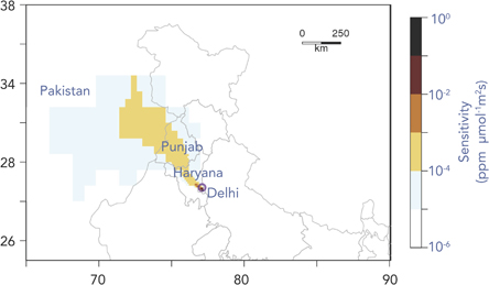
Figure 1. Median 2012–2016 STILT sensitivities of PM2.5 observations in Delhi (28.62°N, 77.21°E, purple circle) to fire emissions in the surrounding grid cells during the post-monsoon burning season (October 17–November 30). Sensitivities below 10−6 ppm μmol−1 m2 s are not shown.
Download figure:
Standard image High-resolution image2. Data and methods
2.1. Surface and satellite observations
The CPCB provides online hourly observations of a variety of pollutants including PM2.5 at 12 sites within Delhi (www.cpcb.gov.in/CAAQM). We focus on observed PM2.5 during the post-monsoon burning season (here defined as October 17–November 30) during 2012–2016. We find that at least 90% of October–November FRP over the northwestern IGP during 2012–2016 is detected during this time window. No CPCB site provides a complete record of PM2.5 observations during the entire course of 2012–2016. The US Embassy in Delhi (https://in.usembassy.gov/embassy-consulates/new-delhi/air-quality-data/) also provides daily PM2.5 from 2013–2016, and is mostly complete during that time span. Finally, we rely on observations from a new monitoring network, #Breathe (http://api.indiaspend.org/dashboard/), launched in 2016 by IndiaSpend, a grassroots initiative to monitor air quality at ten sites in Delhi and elsewhere in India. Figure S1 shows the spatial configuration of all surface sites where PM2.5 was available sometime during 2012–2016. We aggregate and validate these surface observations with satellite AOD (described in section 3.1) retrieved from the MODIS Level 3 Aqua Deep Blue algorithm (MYD08D3; Hsu et al 2013). The Deep Blue algorithm is designed to provide AOD retrievals over bright surfaces, and was found to correlate well with the AERONET station in Kanpur, India (0.70 ≤ R ≤ 0.86; Sayer et al 2013).
2.2. Fire emission inventories
In situ information that can be used to quantify regional fire emissions on the daily scale in Punjab and Haryana is limited. Thus, we consider top-down fire emission inventories that are based on satellite information. The inventories considered in this study are the Fire Inventory from NCAR (FINN; Wiedinmyer et al 2011), the Global Fire Emissions Database version 4 with small fires (GFED4.1s; van der Werf et al 2017, Giglio et al 2013, Randerson et al 2012), the Global Fire Assimilation System (GFAS; Kaiser et al 2012), and The Quick Fire Emissions Dataset (QFED; Darmenov and da Silva 2013). Each of these fire emission inventories are based in part on thermal anomalies detected by MODIS (Giglio et al 2006). However, they each differ in their treatment of emission factors and land cover that translate these thermal anomalies into emission estimates, and they also have different methods for treating gaps in the MODIS record. We include another inventory, called GFED+Agriculture, where increase the GFED4.1s emission factors associated with agricultural burning by a factor of three. More detailed information about each inventory is contained in appendix S1 available at stacks.iop.org/ERL/13/044018/mmedia.
2.3. Particle dispersion, chemical transport, and statistical modeling
We perform 2012–2016 simulations of daily surface PM2.5 in Delhi using the Stochastic Time-Inverted Lagragian Transport (STILT) model (Lin et al 2003), driven by 0.5° × 0.5° Global Data Assimilation meteorology (GDAS; https://ready.arl.noaa.gov/gdas1.php). STILT is a receptor-oriented Lagrangian particle dispersion model (appendix S2), and has been used previously to assess the influence of wildfires on urban air pollution (Mallia et al 2015). Figure 1 shows the spatial footprint of the median 2012–2016 sensitivities of a Delhi receptor (28.62°N, 77.21°E) to the surrounding emissions during the burning season. Sensitivities are derived from particle back-trajectories (appendix S2). We see that Delhi is highly sensitive (~10−3 ppm μmol−1 m2 s) to the upwind burning regions in Punjab. Similar to Koplitz et al (2016), we assume that the PM2.5 reaching Delhi from upwind fires is in its primary BC or OC form.

Figure 2. (Top) Number of daily-averaged PM2.5 observations available at the Central Pollution Control Board (CPCB), US Embassy, and India Spend sites during the post-monsoon burning season (October 17–November 30) for each year during 2012–2016. (Bottom) Correlations R between observed PM2.5 and satellite aerosol optical depth (AOD) over Delhi. The horizontal line at R = 0.5 corresponds to the threshold used to determine if a site is included in the PM2.5 network average. All correlations above R = 0.5 are statistically significant (p < 0.05).
Download figure:
Standard image High-resolution imageUsing STILT footprints, we simulate the urban fate of primary PM2.5 from fires and assume no chemistry. To account for additional PM2.5 production from other anthropogenic sources, we determine a background or baseline from observations (described further in section 3.1). We compare this baseline to a simulated anthropogenic PM2.5 from the 3D global chemical transport model, GEOS-Chem (geos-chem.org; appendix S2).
We tune the STILT simulation of PM2.5 for a certain receptor using the least absolute shrinkage and selection operator (LASSO; Tibshirani 1996, appendix S3), which is a statistical model that here relies on local variables that may not be well captured in the 0.5° reanalysis, e.g. local precipitation, mixing layer height, and wind speed. All variables are taken from the Integrated Global Radiosonde Archive (Durre et al 2006) and the Global Historical Climatology Network (Menne et al 2012).
3. Results
3.1. Creating a network-average and anthropogenic baseline of PM2.5
Due to data inconsistencies among the CPCB sites, we employ data quality preprocessing before calculating a city-wide network average of urban PM2.5 for Delhi. Figure 2 shows the number of daily averaged PM2.5 observations available at each site during the burning season for each year. Few CPCB sites have a record of observations of more than three years during 2012–2016. To represent mean pollution exposure across the city through the years, and account for potential problems with instrumentation or local outliers, we implement a two-step data-cleaning procedure (appendix S4). In 2016, we have data from CPCB, US Embassy, and India Spend PM2.5 observations. We compare each data source (figure S2) and find close correlation between datasets (R = 0.91–0.92).
We next determine a PM2.5 baseline in Delhi to represent typical non-fire anthropogenic pollution levels in the absence of smoke from agricultural fires. Quantification of this baseline is important as we use it to derive a PM2.5 enhancement from observations (yobs = total observed PM2.5—baseline). Baseline anthropogenic PM2.5 in post-monsoon months consists of elemental carbon, organic matter, and secondary sulfate-nitrate-ammonium from gasoline exhaust, coal combustion, dust, and urban biomass combustion (Pant et al 2015). For simplicity, we assume that baseline levels are constant during a given burning season. However, we anticipate that baseline PM2.5 likely changes over the years due to changes in the surface monitoring network and local emission sources. For these reasons, we compute a unique baseline PM2.5 for each year during 2012–2016. We apply three different methods with different assumptions in order to test the robustness of our baseline estimates. Briefly (more details discussed in appendix S5), Method 1 determines the baseline by averaging all observations on the last day of N days of no fires in the Punjab. Method 2 compares overlapping fire and STILT sensitivity grid cells, and determines a baseline if little or no overlap is detected. Method 3 averages the lowest M weekly average PM2.5 observations.
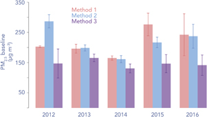
Figure 3. Estimates of the anthropogenic PM2.5 background in Delhi during the burning season (October 17–November 30). Method 1 determines the baseline by averaging all observations on the last day of N days of no fires in the Punjab. Method 2 compares overlapping fire and STILT sensitivity grid cells, and determines a baseline if little or no overlap is detected. Method 3 averages the lowest M weekly average PM2.5 observations. Error bars represent 1 standard deviation when baseline parameters (e.g. N, M) are varied, as described in the text.
Download figure:
Standard image High-resolution imageFigure 3 shows the interannual variability in baseline estimates of urban pollution in Delhi for 2012–2016. Depending on the year and method chosen, the baseline can vary from 130–290 μg m−3. The Method 3 baseline is consistently lower than the other baselines, however each baseline estimate is at least twice the CPCB daily air quality standard of 60 μg m−3. Method 3 shows the greatest interannual stability, and predicts an average baseline across 2012–2016 of about 150 μg m−3, which is within the annual average range of 122.3 ± 90.7 μg m−3 total PM2.5 reported by Tiwari et al (2013) for Delhi in 2011. The mean network averaged PM2.5 during the month prior to the post-monsoon burning season (here September 17–October 16) ranges from 90–150 μg m−3 during 2012–2016, which is slightly lower but near the Method 3 baseline estimate.
We compare these baseline estimates of Delhi PM2.5 to that provided by GEOS-Chem. For this comparison, we perform the GEOS-Chem simulation without the influence of fires. Figure S3 shows the resulting distribution of daily average urban PM2.5 during the burning season of 2012. The distribution is centered on a mean of 99 μg m−3, but is slightly skewed towards larger PM2.5 values, with a maximum at 200 μg m−3. Our observation-driven method for determining the 2012 PM2.5 baseline yields values ranging from 147 ± 47.9 μg m−3 to 287 ± 21.9 μg m−3 (figure 3), or about 1.5–3 times the mean GEOS-Chem simulated baseline.
3.2. Variability of surface PM2.5
We first probe how well the STILT modeling framework reproduces the variability of PM2.5 in Delhi during the burning season. Our approach is to couple daily STILT sensitivity maps to each of the fire emission inventories described in appendix S1 and compare the resulting PM2.5 enhancements in Delhi to those observed when averaged across the network and with the derived PM2.5 baseline subtracted. To reduce noise and variability arising from local emissions, we consider only weekly-averaged modeled and observed PM2.5 enhancements. Results show that each of the emission inventories to some degree captures the variability in the surface observed surface PM2.5 (0.29 < R < 0.50, table 1), suggesting that smoke from fires upwind drives at least part of the weekly variability of Delhi PM2.5. This modeling result agrees with previous studies that report significant correlations between urban AOD, PM10, visibility, and PM2.5 and MODIS FRP (Liu et al 2018, Kaskaoutis et al 2014).
Table 1. Correlation and root mean squared error (RMSE) between modeled and observed PM2.5 enhancements in Delhi for 2012–2016. Ranges are determined by the method (1–3) used to determine the anthropogenic baseline (see section 3.1).
| STILTa | STILT + LASSOb | |||
|---|---|---|---|---|
| Model | Correlation | RMSE | Correlation | RMSE |
| GFED | 0.43–0.50 | 80–109 | 0.72–0.78 | 53–62 |
| QFED | 0.41–0.46 | 79–101 | 0.69–0.72 | 59–65 |
| FINN | 0.29–0.45 | 80–98 | 0.70–0.73 | 59–64 |
| GFAS | 0.38–0.42 | 81–109 | 0.66–0.70 | 62–68 |
aCorrelation and RMSE between observed and modeled PM2.5. The PM2.5 enhancements are simulated using the Stochastic Time-Inverted Lagrangian Transport (STILT) model driven with several fire emission inventories. bCorrelation and RMSE between observed and modeled PM2.5. Here the results from STILT are combined with local observed meteorology from sondes (precipitation, wind speed, wind direction, mixing height) and fit to the observed PM2.5 enhancements using the least absolute shrinkage and selection operator (LASSO), a form of regularized linear regression.

Figure 4. Standardized regression coefficients (μg m−3 standard deviation−1) fit to daily PM2.5 enhancements, derived from three different baseline methods. See text for description of these methods. The GFED term is the PM2.5 prediction based on driving STILT with GFED4.1s. The other predictors are derived from surface or sonde observed meteorology.
Download figure:
Standard image High-resolution imageAs a measure of the mean bias of our predicted PM2.5 compared to Delhi observations, we compute the root mean squared error RMSE (table 1). We find that driving the model with STILT alone accounts for an RMSE between 79–109 μg m−3, depending on the baseline method and emissions inventory, revealing that even though we can predict much of the observed surface PM2.5 variability using STILT, we greatly underestimate the magnitude of the enhancements. A potential reason for this underestimate could be that the GDAS reanalysis used to drive STILT poorly characterizes the local meteorology. We add information from local meteorological sources and fit a statistical model to the observed PM2.5 enhancements. Results of the statistical model are shown in table 1. Adding local meteorological factors improves the correlation of predicted vs. observed PM2.5 in each fire emission scenario (0.66 < R < 0.78). Figure 4 presents the normalized regression coefficient weights for just the GFED4.1s simulation. Regression coefficients for other statistical models fit with different emission inventories are shown in figure S5. The STILT-GFED4.1s predictor is one of the most significant contributors, as expected by the presence of significant correlation (0.43 < R < 0.50) between observed and GFED4.1s STILT-derived PM2.5 enhancements. The next two dominant predictors of observed PM2.5 are wind speed below the boundary layer and precipitation. This result underscores the importance of local meteorology as drivers of urban PM2.5 variability and suggests that the assimilated GDAS meteorology may not capture such meteorological effects at 0.5° resolution. The statistical model yields RMSE values ranging from 53–68 μg m−3, substantially lower than those from the purely STILT-driven model, but still rather large. We hypothesize that other unaccounted factors (e.g. the smoke from small fires that escape satellite detection) could lead to model bias. We discuss this reasoning further in section 4.
3.3. Maximum daily enhancement of PM2.5 during burning season
While we capture the variability of PM2.5 with both STILT and the statistical model, in both cases we find a high RMSE when compared to observations. Here we focus on smoke extremes during each fire season to probe whether the model systematically underestimates surface PM2.5. We also quantify the contribution of smoke PM2.5 derived from observations or STILT to total PM2.5 during these extreme events.
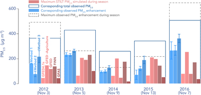
Figure 5. The maximum of daily simulated enhancements of PM2.5 due to fires upwind fires during each post-monsoon burning season. In parentheses is the day in which the STILT simulation of PM2.5 reached its maximum during each burning season from 2012–2016. In shades of red are the different model simulated PM2.5 enhancements using different fire emission inventories that correspond to the date in parentheses. In shades of blue are the different network-averaged observed PM2.5 enhancement estimates above the anthropogenic baseline for three different baseline methods that correspond to the date in parentheses. The outlined dark blue box represents the total observed PM2.5 for the date in parentheses. The outlined grey box represents the maximum observed PM2.5 enhancement regardless of the date when the STILT simulation predicted largest enhancement during the post-monsoon burning season.
Download figure:
Standard image High-resolution imageFigure 5 shows the model simulated maximum daily smoke enhancement in each burning season—i.e. the enhancement on that day each season characterized by the greatest simulated PM2.5 value. For years when STILT simulations disagree on which day should produce maximal PM2.5, we choose the day for which most models agree. The plot also shows the observed PM2.5 enhancement and total observed PM2.5 that correspond to the day where the STILT simulation predicted the maximal urban pollution enhancement. We compare these values in figure 5 to the maximum observed PM2.5 enhancement for each burning season, regardless of when the STILT simulation predicted a large enhancement. The largest observed PM2.5 enhancements occur in 2012 and 2016 (492 and 648 μg m−3 respectively, averaged across all baseline methods). The maximum observed enhancements are much lower during 2013–2015 (130–264 μg m−3), which could be a result of lower fire activity or other local pollution-causing events. The magnitude and interannual variability in the maximum observed PM2.5 enhancement differs from STILT, for which the largest simulated PM2.5 enhancement occurs in 2013 (65–232 μg m−3). The STILT simulated enhancements show roughly interannual consistency during 2012–2016 when averaged across all inventories (99–160 μg m−3). However, several of the days over 2012–2016 where the observations alone predict the largest seasonal enhancements are not consistent with the days STILT predicts. When we instead compare the maximum STILT enhancements to the same-day corresponding observed PM2.5 enhancement (108–299 μg m−3), we find closer agreement. The FINN and GFED + Agriculture emission inventories often give the largest estimate of magnitude of the PM2.5 enhancement in Delhi (145–231 μg m−3 and 147–255 μg m−3, respectively). We find the largest mismatch between observed and modeled enhancements during 2012 and 2016 across all models. In these years, depending on emission inventory, the maximum STILT derived enhancements are 45–147 and 37–255 μg m−3, respectively.
Table 2. The percentage of the maximum PM2.5 simulated STILT enhancements to corresponding total observed PM2.5 for each burning season in Delhi during 2012–2016. OBS refers to the range of PM2.5 enhancements derived using the three baseline methods (see section 3.1). Each of the other columns reports simulated PM2.5 enhancements from STILT.
| Maximum enhancement | ||||||
|---|---|---|---|---|---|---|
| Year | OBSa | GFED | GFED + AGRIb | QFED | FINN | GFAS |
| 2012 | 21%–60% | 13% | 40% | 33% | 38% | 12% |
| 2013 | 54%–61% | 15% | 48% | 45% | 54% | 24% |
| 2014 | 36%–50% | 24% | 78% | 18% | 68% | 7.0% |
| 2015 | 21%–56% | 19% | 62% | 58% | 42% | 15% |
| 2016 | 52%–72% | 16% | 50% | 16% | 34% | 7.3% |
aOBS corresponds to the network-averaged PM2.5 enhancement that was observed on same day that the maximum STILT-simulated PM2.5 enhancement occurred. bGFED+AGRI is an emissions inventory based on GFED dry matter emissions, with 100% agriculture landcover assumed and emissions factors increased by a factor of three.
Table 2 shows the percent contributions of smoke PM2.5 to total PM2.5 on extreme smoke days predicted by STILT—i.e. the day during the season where STILT predicts that the smoke enhancement is greatest. This provides a metric of the contribution of fires during the largest predicted episodes each season to total surface particulate pollution observed in Delhi. The observed PM2.5 enhancement on days when STILT predicted a pollution maximum accounts for 21%–72% of the total observed PM2.5, depending on the year and baseline method used, implying that PM2.5 from a regional source (here assumed to be fires) can constitute a large fraction of the total PM2.5 concentration. For STILT PM2.5, the GFED + Agriculture and FINN simulations provide large PM2.5 estimates, and can account for as much as 78% and 68% percent of the total corresponding observed PM2.5 in 2014, respectively. In other years, these two inventories can account for as much as and 40%–62% and 28%–54% of the total corresponding observed PM2.5, respectively. This result means that on days when STILT predicts a large enhancement in Delhi from agricultural fires, the smoke from these fires constitutes a large portion of the total PM2.5. On the lower end, the GFAS simulation accounts for just 7.0%–24% of the corresponding total PM2.5. Since all inventories use MODIS fire detections to constrain emissions, the variability in PM2.5 estimates that arise from these inventories can be attributed to differing emission factors, allocation of additional fires from burned area maps, model assimilation, and MODIS gap-filling methods. Figure 5 and tables 1–2 show the large sensitivity in our PM2.5 estimates to the underlying assumptions used to translate satellite retrievals to actual emissions.
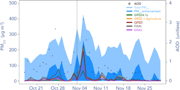
Figure 6. Time series of observed and modeled PM2.5 during the 2013 burning season. The blue envelopes represent the observed total PM2.5 and the PM2.5 enhancement derived by subtracting the daily PM2.5 by the mean PM2.5 of the lowest week during the season. Each colored line represents a model simulation with a different fire emission inventory. The black dots are the MODIS AOD retrievals during the burning season. The dashed vertical line on represents the start of the Diwali festival for 2013 (November 3rd).
Download figure:
Standard image High-resolution imageThe results of figure 5 and table 2 show that STILT can at times reproduce much of the observed PM2.5 enhancement in Delhi (depending on the emission inventory used), a result that appears at odds with the very high RMSE between observed and modeled enhancements in table 1. To further investigate the reasons driving the discrepancies between observed and modeled PM2.5 enhancements, we plot the time series of observed and simulated PM2.5 enhancements for the 2013 post-monsoon burning season (figure 6). We show observed and simulated PM2.5 for 2012 and 2014–16 in figure S5 and include the daily GEOS-Chem simulation of PM2.5 for 2012. For 2013, three versions of the STILT model—those driven by FINN, QFED, and GFED + Agriculture emissions—are able to match the PM2.5 enhancement on November 5th almost exactly. However, during the days before and after this large pollution enhancement, these models predict little or no PM2.5.
There are several potential reasons for the mismatches between modeled and observed enhancements in smoke PM2.5. On the days preceding the November 5th maximum, MODIS may have been unable to detect many small agricultural fires upwind. Only when a sufficient number of these small fires become detectable is a pollution enhancement predicted by the STILT model. The challenge in detecting small fires from satellites is a well-known problem (Randerson et al 2012). November 3rd was also the start of Diwali in 2013, a Hindu religious holiday celebrated with an abundance of firecrackers and sparklers. However, we find that although it can be a contributor, Diwali is not a principal driver of sustained post-monsoon PM2.5 enhancements (appendix S6). For the days succeeding the November 5th PM2.5 enhancement, local meteorology may have deviated from the coarser 0.5° GDAS winds, favoring increased stagnation within the city and potentially amplifying surface PM2.5 exposure. Stagnation could have been further amplified by boundary layer stabilization from enhanced PM2.5 aloft, a feedback previously examined as an amplifier of pollution in China (e.g. Petäjä et al 2016, Wang et al 2014, Ding et al 2016).
We also hypothesize that dense smoke from fires may sometimes obscure the signal of fire activity at the earth's surface. Figure 7(a) shows True Color Terra reflectance imagery from MODIS as well as MODIS Aqua + Terra fire detections on a sample day over the IGP (November 6, 2016). Figure 7(b) shows the Visible Infrared Imaging Radiometer Suite (VIIRS) reflectance imagery with VIIRS fire detections. VIIRS detects many more fires on this day than does MODIS, perhaps because VIIRS has a finer resolution and different fire detection algorithm than MODIS (375 m compared to 1 km; Schroeder et al 2014). The MODIS cloud product misidentifies the thick smoke plumes over the Punjab as clouds on this day. The Collection 6 MODIS fire product accounts for thick smoke from fires by relaxing the thresholds that determine whether a pixel is cloud-obscured (Giglio et al 2016). In fact, on the day illustrated in figure 7 (November 6th, 2016), the MODIS fire product assumes that no pixels over Punjab and Haryana are obscured by clouds, even though the MODIS cloud product reports cloud cover (figure 7(c)). Even so, fire detections still appear minimal in regions where the smoke is thickest. Thus we hypothesize that the large model underestimates of smoke PM2.5 enhancements in 2016 may be due in large part to layers of dense smoke interfering with satellite detection of thermal anomalies.

Figure 7. MODIS or VIIRS surface reflectance maps for November 6, 2016 overlaid with different fire and cloud detection algorithms. The top panel (A) shows the Terra and Aqua MODIS 1 km fire counts used in part to drive the fire emission inventories used in this paper. The middle panel (B) shows 375 m VIIRS day and night fire detections. The third panel (C) shows MODIS fire detections with MODIS Terra daytime cloud fraction overlaid. Comparison of the top and middle panels show that the resolution of the satellite sensor could influence the number of fires detected, meaning that many smaller fires may be undetected with current MODIS capabilities. Comparison with the bottom panel shows that thick smoke in the Indo-Gangetic Plain may be detected as clouds, which may interfere with surface thermal anomalies.
Download figure:
Standard image High-resolution image
4. Discussion
We estimate the contribution of smoke from upwind agricultural fire emissions to PM2.5 exposure in Delhi during the burning season (October 17–November 30). We apply two methods: (1) an observationally based method using CPCB and other surface observations, in which we determine daily enhancements above background levels, averaged over Delhi, and (2) application of the Lagrangian particle dispersion model STILT, in which we implement a suite of fire emission inventories. We find that the two approaches yield timeseries of weekly-averaged PM2.5 that correlate significantly (0.29 < R < 0.50) with each other, implying that smoke from agricultural fires upwind accounts for much of the weekly variability of PM2.5 in Delhi during the burning season. Addition of local meteorological factors (precipitation, wind speed, wind direction, temperature, and mixing heights) improves the correlation further (0.66 < R < 0.78). The maximum PM2.5 smoke concentration calculated by the STILT model during each burning season is of similar magnitude as its corresponding observed PM2.5 enhancement. For example, in 2013, the maximum simulated PM2.5 enhancements (occurring on November 5th) from GFED + Agriculture, QFED, and FINN are 48%, 45%, and 54% of the corresponding observed maximum PM2.5, respectively, close to the 54%–61% range derived from observations (table 2). This result implies that smoke from agricultural fires contributes significantly to PM2.5 pollution in Delhi during intense episodes. However, in general, the PM2.5 simulations greatly underestimate the enhancements implied by the observations over the entire burning season, with RMSE of 79–109 μg m−3, indicating that further improvements to fire emission inventories are needed.
We find that although we can predict the magnitude of the maximum PM2.5 enhancement during most seasons using STILT, we miss many smaller PM2.5 enhancements. In the case of 2013, many smaller fires were likely undetected due to limitations in the resolution of the MODIS retrieval. Active fire detection using higher resolution (375 m) VIIRS data may provide a promising new avenue to quantify the contribution from small fires. For other fire seasons, as in 2016, STILT underestimates the maximum PM2.5 enhancement more severely, even though Delhi experienced much greater concentrations of PM2.5 than compared to previous seasons. The fires in 2016 were especially strong, but analysis of visual MODIS imagery, fire counts, and cloud cover suggests that many fires were either missed due to the coarse resolution of MODIS detection or were not observed by satellites due to interference of thick smoke. If there are missed fires due to the interaction of thick smoke with surface thermal anomalies, this could potential represent a large source of underestimation in assimilated fire emission inventories. As GFAS and QFED estimate FRP in cloud-obscured pixels by using information from adjacent non-obscured pixels, an omitted or false-negative thermal anomaly under thick smoke would not be assimilated in the fire emission inventory. In Punjab and Haryana, where thick smoke is prevalent during the post-monsoon season due to agricultural fires and low boundary layers, this problem could particularly exacerbate low fire emission estimates.
Some uncertainty in this analysis can be traced to the methods of obtaining a seasonal PM2.5 baseline. We incorporate three different methods to isolate the PM2.5 enhancement due to fires. However, each of these methods shows considerable sensitivity to its various threshold parameters, and there is much variability between each of the methods (e.g. the baseline for 2016 ranges from 140 to 240 μg m−3). As more monitors become available in Delhi, distinguishing a regional signal from local enhancement will become less challenging. Inversion methods to optimize emission factors or the spatial allocation of emissions could then be applied with more confidence, since these methods rely on the accuracy of the observed PM2.5 enhancement. Instead of computing the baseline from the observations, one could instead simulate the PM2.5 baseline using a chemistry model such as GEOS-Chem over the entire time domain. However, the result of such simulations would depend strongly on the quality of the emissions used to drive the model and on the extent to which we understand pollution chemistry in this region. In our 2012 GEOS-Chem simulation, we find that the model underestimates the PM2.5 baseline by at least a factor of 2, compared to the baselines derived from observations.
Many studies have assessed the human health impact of elevated particulate pollution in Delhi (Nagpure et al 2014, Kandlikar and Ramachandran 2000). Our work builds on these studies by quantifying the contribution of agricultural burning in the Punjab and Haryana to the degradation of Delhi air quality. Although officially banned nationally and enforced on the state level by the National Green Tribunal Act of 2010 (Nain Gill 2010), the practice of agricultural burning is cheap and commonplace for farmers after harvest. India's population is expected to surpass China 2022, and reach 1.7 billion by 2050 (United Nations 2015). Delhi is projected to grow to a population of 36 million by 2050 (Hoornweg and Pope 2013). Thus the need for efficient and inexpensive agricultural production is paramount to feeding the increasing population. However, the adverse effects of fire emissions need to continue to be seriously considered and more accurately quantified as the populations of Delhi and the greater IGP continue to grow, leaving more people at risk. Building on the approaches in previous studies (e.g. Liu et al 2018), the modeling approach presented in this paper can be used to infer not just the co-variability of urban pollution and upwind fires, but also the percent contribution of smoke to the already intense urban PM2.5 in Delhi. As estimates of fire emissions improve and the distribution of air quality monitors in Delhi expands, such an approach will reduce uncertainty in the impacts of current agricultural practices that involve fire. This information can provide policymakers with a quantitative sense of the consequences of current agricultural burning practices in regions upwind of the city in order to inform decision-making.