

Abstract
Widespread, drought-induced forest mortality has been documented on every forested continent over the last two decades, yet early pre-mortality indicators of tree death remain poorly understood. Remotely sensed physiological-based measures offer a means for large-scale analysis to understand and predict drought-induced mortality. Here, we use laser-guided imaging spectroscopy from multiple years of aerial surveys to assess the impact of sustained canopy water loss on tree mortality. We analyze both gross canopy mortality in 2016 and the change in mortality between 2015 and 2016 in millions of sampled conifer forest locations throughout the Sierra Nevada mountains in California. On average, sustained water loss and gross mortality are strongly related, and year-to-year water loss within the drought indicates subsequent mortality. Both relationships are consistent after controlling for location and tree community composition, suggesting that these metrics may serve as indicators of mortality during a drought.
Export citation and abstract BibTeX RIS

Original content from this work may be used under the terms of the Creative Commons Attribution 3.0 licence.
Any further distribution of this work must maintain attribution to the author(s) and the title of the work, journal citation and DOI.
Corrections were made to this article on 5 January 2018. Extra acknowledgments were added.
1. Introduction
With the increased prevalence and severity of hot droughts, our ability to anticipate tree mortality has grown in importance to forest ecology and management. A growing body of literature indicates that the frequency and impact of hot droughts are increasing as the planet warms (Overpeck 2013, AghaKouchak et al 2014, Cook et al 2014. With an increased frequency of hot droughts comes risk to forests. At the planetary scale, global warming is likely to raise background rates of mortality and die-off within forests (van Mantgem et al 2009, Allen et al 2010). Critically, drought stress has been shown to increase the vulnerability of most forest biomes to drought, irrespective of precipitation levels (Choat et al 2012). However, the full extent of forest vulnerability to water stress remains unknown.
Multiple studies have demonstrated that remotely sensed metrics can be used to describe different forest mortality events, including piñon-juniper forest die-offs in the Interior West of the US in 2002–2003 (Breshears et al 2005), aspen forest mortality in Colorado from 2009–2011 (Huang and Anderegg 2012), and semiarid subtropical dry zone canopy loss in Texas in 2011 (Schwantes et al 2016). To our knowledge, however, remote sensing techniques have not yet demonstrated the ability to predict mortality risk from water stress and other drought-related factors in advance. Consequently, we explore the influence of remotely sensed canopy water content (CWC), a measure of tree physiological response to drought (Asner et al 2016), on tree mortality in order to examine a more direct link between drought and mortality.
Risks from hot drought are particularly relevant to the US state of California. In recent years California has been victim to its most severe drought in over a millennia (Griffin and Anchukaitis 2014). Remote sensing has been used to quantify the impact of California's 2012–2016 drought, indicating that 58 million large trees had suffered severe water stress by 2015 (Asner et al 2016). Tree mortality from this drought has been particularly acute in dense stands and in forests where the 35 year mean annual climatic water deficit or CWD has been high (Young et al 2017). Tree mortality rates have been demonstrated to be species specific within regions of the Sierra Nevada, and have been shown to be correlated with multiple, spatially nested environmental variables (Paz-Kagan et al 2017 in press). Given the increasing probability of warm-dry conditions in California due to anthropogenic warming (Diffenbaugh et al 2015), understanding how water stress is linked to future tree mortality across a broad range of forest types is important for forest management, conservation, and resource policy (Edmund G Brown 2015).
We aimed to predict mortality in conifers throughout the Sierra Nevada mountain region using changes in remotely sensed CWC. We asked (1) can we use remotely measured changes in water stress to predict gross tree mortality over the course of a drought, and (2) can changes in CWC between years be used to predict future mortality in an ongoing drought? We used high-fidelity, laser-guided imaging spectroscopy data from flights in 2015 and 2016 to identify mortality throughout the Sierra Nevada, as well as to derive changes in annually modeled CWC between 2010 and 2016. The broad sampling coverage achieved through remote sensing allowed us to determine robust links between CWC decline and tree mortality that proved consistent across both space and tree community.
2. Materials and methods
We combined multiple data sets with different native spatial resolutions in order to link CWC declines through time with increases in tree mortality. The first data set is composed of 2 m resolution imaging spectroscopy and LiDAR data from spatially overlapping collections in August 2015 and July 2016. These data were used to identify live and dead tree cover in both years. The second data set is a 30 m resolution CWC time series from 2010–2016 (excluding 2012). The CWC time series is generated using a deep-learning model which relates a suite of satellite and terrain data to CWC observed during the flights in 2015 and 2016, and is then used to retrospectively model CWC from 2010–2014 (Asner et al 2016). This section will first describe the flight data collection, followed by a detailed discussion of both data sets, and then conclude with a description of the analysis techniques applied to the data.
2.1. Data collection
High-fidelity imaging spectroscopy (HiFIS) and LiDAR data were collected by the Carnegie Airborne Observatory (CAO) throughout California in both August 2015 and July 2016. The HiFIS and LiDAR are obtained using the Airborne Taxonomic Mapping System (AToMS), which is carried onboard a Dornier 228 aircraft (Asner et al 2012). The HiFIS spectral data were collected in 427 channels over the 350–2485 nm wavelength range in 5 nm increments (full-width at half max). The data were collected from approximately 2000 m above ground level, corresponding to a 2 m ground-level spatial resolution. We transformed the HiFIS data from radiance to apparent surface reflectance, and applied a bidirectional reflectance distribution function to correct for collection artifacts (Asner et al 2012). The LiDAR data covered a similar ground-level swath with a density of approximately 4 laser shots per square meter, obtained using a 34° field of view, a pulse repetition frequency of 50 kHz per laser, and a beam divergence of 0.56 mrad per laser. The LiDAR data were used to derive tree canopy height at 1 m ground-level resolution (later averaged to 2 m to match the HiFIS data) (Lefsky et al 1990), as well as an inter-canopy shade mask for the HiFIS data at 2 m ground-level resolution (Asner et al 2007).
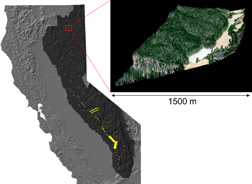
Figure 1. Locations with HiFIS and LiDAR data from both 2015 and 2016 (yellow), totaling 26 706 ha made up of 59.7 million 2 m ground-level resolution data points. The area shown in dark gray is designated as the Sierra Nevada Conservancy by the State of California (Schwarzenegger 2004, State of California 2017). The inset plot shows the 2 m ground-level resolution RGB reflectance overlaid on the LiDAR for a single intersection of the 2015 and 2016 flight data.
Download figure:
Standard image High-resolution image
Figure 2. NDVI histograms of conifers within the Sequoia and Kings Canyon National Parks. The live and dead classifications were determined by (Paz-Kagan et al 2017). The threshold of 0.4 used to classify mortality in this work is drawn in black on top of the histogram.
Download figure:
Standard image High-resolution image
Figure 3. Illustration of the procedure used to classify each NDVI pixel (2 m ground-level resolution) within each CWC pixel (30 m ground-level resolution). Black pixels indicate areas that are either shaded in one of the two years, or where the tree canopy height is below 5 m. Following the classification, we calculate the mortality fraction within each CWC pixel.
Download figure:
Standard image High-resolution imageTo measure changes in mortality, we used all locations where data were collected in both the 2015 and 2016 flights throughout the Sierra Nevada. Most sampling flights were oriented North–South in 2015 and with a 46 degree counter-clockwise rotation in 2016, resulting in a large number of intersections scattered throughout the Sierra Nevada (figure 1). The inset in figure 1 demonstrates that each intersection location, while small with respect to California, includes many hundreds of thousands of individual grid cells. Some specific areas of interest, such as Sequoia National Park, were measured thoroughly in both years, leading to a higher level of intersected coverage.
We limited this study to the Sierra Nevada mountain region or 'conservancy' (Schwarzenegger 2004, State of California 2017). We also excluded any location where a fire occurred between 2010 and 2017 (USGS 2016). To focus specifically on conifers, where we believe major direction shifts in NDVI (which we use to indicate mortality) are less likely to be phenological, we used the CALFIRE FVEG database to delineate conifer forest cover (CALFIRE FRAP 2015). We selected only pixels where the California Wildlife Habitat Relationships (CWHR) system indicated a conifer habitat (i.e. a conifer community), with no oaks listed as primary species (CDFW 2014). The set of conifer communities used, and the dominant species within each, are shown in table S1. Finally, we selected pixels where the canopy exceeded 5 m in height, and which were not shaded by the surrounding canopy in either the 2015 or the 2016 flight. In total this resulted in 26 706 ha of data with coverage in both 2015 and 2016, with over 59.7 million individual grid cells at 2 m ground-level resolution.
2.2. Mortality measurements
We use the term mortality to indicate portions of a canopy where the foliage dropped below an NDVI of 0.4. The NDVI was calculated from the HiFIS data using 10 nm wide reflectance bands centered at 680 and 800 nm, after excluding shaded areas and vegetation of less than 2 m in height. To select this threshold, we examined mortality classification maps of 13 000 ha of Sequoia and Kings Canyon National Parks presented in Paz-Kagan et al (2017) in press. The mortality maps in Paz-Kagan et al were constructed using HiFIS and LiDAR data from the 2015 flights, and were demonstrated to be 99% accurate in identifying actual full-tree mortality observed in the field. Figure 2 shows a histogram of NDVI of the conifers within the study area for both live and dead classes (normalized to a maximum of one). To be conservative when classifying mortality, we selected an NDVI threshold of 0.4, which corresponds to a dead misclassification rate of less than 1% and a live misclassification rate of 32%. Using an NDVI threshold to determine mortality allows for the classification to be extended beyond the Sequoia and Kings Canyon National Parks in a computationally efficient manner, and without the introduction of potential artifacts caused by using a complex model outside of the sample area.
Figure 3 illustrates a set of example NDVI data within the extent of a single CWC time series pixel, and demonstrates how we classified the NDVI and rectified the difference in resolution between the mortality classification (2 m), and the CWC time series (30 m). First, we applied the NDVI threshold of 0.4 to all unmasked pixels in both the 2015 and 2016 data. We then calculated the mortality fraction of both the 2015 and 2016 as

where M is the mortality fraction, p is the mortality classification of each 2 m pixel, s is a binary mask with a value of 1 if the pixel is excluded (due to shade or insufficient height), and Cp is the set of 2 m resolution pixels within a given CWC pixel. We then calculate the mortality increase, ∆M, as
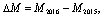
where the subscript indicates the year. As defined above, a positive ∆M means an increase in mortality, while a negative ∆M indicates foliar growth and/or recovery. Both ∆M and M2016 are used as independent variables in the predictions, and are calculated for each CWC time series pixel. It is important to note that M, and consequently ∆M, is a measurement of mortality fraction, indicating the number of pixels that are below the NDVI threshold of 0.4. This fraction is distinct from the fraction of dead individual trees, as it may include partial foliar dieback.
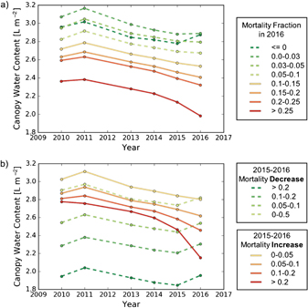
Figure 4. Canopy water content through time for different mortality fractions in 2016 (a) and for different levels of mortality change between 2015 and 2016 (b). Each point represents the mean CWC of all data points within the denoted mortality fraction (a) or mortality fractional change (b) for a given year. In total 26 706 ha of data are included.
Download figure:
Standard image High-resolution image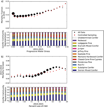
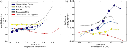
Figure 5. Relationships between progressive water stress from 2011 to 2015 and mortality fraction in 2016 (a) and between percent difference in canopy water content between 2014 and 2015 and the fractional mortality increase between 2015 and 2016 (b). The dot size in the top plot shows the relative quantity of data within each bin (approximately 300 000 data points were used in total). Controlled sampling, shown by the red dots, was performed using Latin Hypercube Sampling over space and conifer community. The bar graphs at the bottom of (a) and (b) show conifer community representations corresponding to each average point immediately above.
Download figure:
Standard image High-resolution image2.3. CWC time series
Canopy water content, or CWC, is the amount of liquid water in the canopy in volumetric and/or mass units, and can be estimated based on spectral absorption features (Gao and Goetz 1990, Ustin et al 1998, Green et al 2006). We calculate CWC from HiFIS data using the software package ACORN (Green 2001), which produces CWC during the atmospheric correction process. The retrieval of CWC from the spectra is performed by ACORN through an iterative method which isolates both the quantity of water vapor in the atmosphere between the sensor and the ground as well as the amount of liquid water in the canopy (CWC) (Gao et al 2009). In Asner et al (2016), we introduced the concept of using changes in CWC through time as a remotely sensed indicator of the physiological response of trees to drought.
In order to examine the CWC in years prior to 2015, we used a sequence of modeled CWC maps produced from 2010 through 2016 (excluding 2012) as in (Asner et al 2016). This time series of CWC was generated by training a deep-learning model to correlate a suite of GIS data, including satellite (Landsat), terrain, and location information, to the CWC of each year, as in (Asner et al 2016). CWC in each year corresponds to the July-August time period. CWC from 2012 is excluded due to the gap between Landsat 5 and Landsat 8 coverage. The CWC time series in this work is updated from (Asner et al 2016) to incorporate training data from the 2016 flights as well, and as such the root mean squared error of CWC predictions on holdout data sets from both years is below 0.35 L m−2, and the r-squared of the modeled versus measured data exceeds 0.88. More detail about the development and application of the deep learning model is available in the supplementary information available at stacks.iop.org/ERL/12/115013/mmedia.
2.4. Controlled Sampling
While much of the intersected flight data are well distributed throughout the Sierra Nevada, several areas of interest have significantly greater representation than others (as shown in figure 1). Consequently, in addition to performing our analysis on the entire intersected dataset, we also used a controlled sampling technique to normalize for the influences of space and conifer community. We drew random points using a Latin Hypercube Sampling method with dimensions of space (north-south and east-west) and community (Swain et al 1992). Each spatial dimension was split into ten evenly divided sections, across the entire extent of samples collected. Within each spatial-dimension bin, and within each conifer community, we drew 200 randomly selected points. In locations where an insufficient number of data points was available, the maximum number available were used. This method allows us to control for the influences of a particular conifer community or spatial region and prevent over-representation.
2.5. Analysis
In order to examine the relationship between a CWC time series and tree mortality, we performed two basic analysis on all data points with CWC and mortality data from both 2015 and 2016, approximately 300 000 data points at the final 30 m resolution. First, to determine which portions of the time series were relevant for further investigation, we divided the data into 8 evenly spaced classes based on M2016. We then averaged all CWC values within each year and within each M2016 class and plotted the results, in order to examine trends through time. This process was then repeated with the classes based on ∆M.
Based on these results, presented below, we then selected two metrics to explore further: progressive water stress (PWS) between 2011 and 2015, and the percent difference in CWC between 2014 and 2015 (%∆ CWC14−15). PWS is calculated by summing the absolute value of the per-pixel percent losses in CWC between 2011 and 2013, between 2013 and 2014, and between 2014 and 2015, as in Asner et al (2016). We split the data into 20 evenly spaced bins based on PWS, and plotted the mean PWS and mean M2016 for each. Additionally, we examined the distribution of conifer communities within each bin, and plotted those on the same axis. This analysis was then repeated for %∆ CWC14−15 and ∆M. Finally, we examined both of these relationships (PWS and M2016 as well as %∆ CWC14−15 and ∆M) on a conifer-community specific level for the five most prevalent conifer communities.
3. Results
Figure 4(a) shows the changes in CWC for different mortality fractions in 2016. CWC generally decreases across all classes of M2016 throughout the drought (2011–2016). Except for the lowest mortality class (where regrowth occurred), trees with lower levels of CWC exhibit higher rates of M2016. We also observe that the classes with the greatest decreases in CWC through time appear to have the greatest increase in M2016. Figure 4(b) shows even more distinct patterns of CWC through time for different classes of ∆M. The strong relationship between changes in CWC from 2015 to 2016 and ∆M is expected given that after mortality, the CWC of a tree declines towards zero. More interesting, however, is that the change in CWC from 2014 to 2015 also appears to be related to increases in mortality, motivating further exploration of %∆ CWC14−15 as an indicator of ∆M.
We examine the relationship between PWS from 2011 to 2015 and M2016 in figure 5(a). The additional change in PWS between 2015 and 2016 is excluded in order to specifically examine the predictive, rather than the descriptive, influence of PWS on M2016. To create figure 5(a), we split the range of observed PWS values into 20 bins, and present the mean PWS and M2016 for each. Figure 5(a) shows a strong positive trend between PWS and M2016, though the trend fails at low levels of PWS due to mortality events unrelated to water stress. These relationships are consistent when considering all data and when using the controlled sampling method (section 2.4). The conifer community representation of all pixels within each PWS bin, shown in the bottom plot of figure 5(a), shows a greater representation of the Closed-Cone Pine-Cypress community, and a lower representation of the Subalpine Conifer community with increasing PWS and M2016.
In figure 5(b), we investigate the relationship between %∆ CWC14−15 and ∆M. We observe a base ∆M rate of about 1% which expands to a mortality rate of approximately 5% with increase %∆ CWC14−15. While this relationship, like that observed in figure 5(a), is robust under controlled sampling, there is a higher degree of deviation in ∆M at high rates of %∆ CWC14−15. This suggests that some spatial regions or conifer communities have higher increases in mortality under water stress. A significant shift in community representation is also evident in figure 5(b), with the Sierran Mixed Conifer community becoming significantly more prevalent and the Red Fir community becoming less prevalent as %∆ CWC14−15 increases.
Figure 6. Relationships between progressive water stress from 2011 to 2015 and mortality fraction in 2016 (a) and between the percent difference in canopy water content between 2014 and 2015 and the fractional mortality increase between 2015 and 2016 (b) for each of the five most common conifer communities in the sampled data. Dot size shows the relative quantity of data at each point (approximately 218 000 data points were used in total).
Download figure:
Standard image High-resolution image
To investigate community-specific mortality fraction trends, we show the same relationships between PWS and M2016 as well as between %∆ CWC14−15 and ∆M for the five most prevalent conifer communities independently in figure 6. While each conifer community has a strong increase in M2016 at high levels of PWS, the trends at lower PWS are quite distinct (figure 6(a)). The Ponderosa Pine community shows a particularly strong relationship between PWS and M2016, which is consistent with expectation (Ganey and Vojta 2011). The Closed-Cone Pine-Cypress community, however, shows an almost inverse relationship between PWS and M2016, indicating a much more substantial tolerance to sustained water loss. The relationships between water stress and mortality within a drought shown in figure 6(b) are different from the community-specific relationships of long-term drought stress in figure 6(a). Sierran Mixed Conifers, which are by far the most prevalent conifer community in our data, show significant increases in ∆M with increasing %∆ CWC14−15. In contrast, the Closed-Cone Pine-Cypress community shows a slight inverse relationship and very little change in ∆M.
4. Discussion
Our results indicate that progressive water stress estimated from remotely sensed data is a strong correlate with gross conifer mortality over the course of a drought within the Sierra Nevada. Independent work has demonstrated a relationship between mortality and a climatological indicator (climate water deficit) at coarse resolution (~4 km) (Young et al 2017). By using remotely sensed measurements of changes in canopy water content, rather than measures of climatological metrics (which indicate a potential for canopy water content changes), we generate a more direct examination of the physiological response of trees to drought. Additionally, by using 30 m resolution data, we are able to examine spatially explicit relationships between mortality and sustained water stress in different conifer communities. Despite the clear overall relationship between mortality and progressive water stress (PWS), we found dramatically different patterns within different conifer communities, ranging from severe rates of mortality with increasing PWS in the Ponderosa Pine community, to almost no relationship in the Closed-Cone Pine-Cypress community. These findings give quantitative support to qualitative claims that trees with high PWS are more vulnerable to mortality (Asner et al 2016).
We also demonstrate that changes in CWC during drought are strongly related to subsequent tree mortality (figures 5(b) and 6(b)). Critically, this relationship is predictive in that the remotely sensed observations indicated where mortality will occur in the future, not simply where it has already occurred. However, we do not claim that high fractional changes in CWC necessarily lead to mortality in subsequent years; rather, high fractional changes in CWC lead to increased vulnerability to future mortality. In the absence of continued environmental stress, it is not certain that trees stressed from drought would subsequently die. It is also significant to note that drought itself is only one of several potential mechanisms of mortality (Meddens et al 2015). In many cases, drought induces stress within trees, which then succumb to death due to attacks from bark beetles (Breshears et al 2005, Raffa et al 2008). Consequently, while changes in CWC may facilitate conditions that lead to mortality, water stress alone is often not the cause of mortality which leads to further uncertainty when predicting future mortality events.
At the highest levels of water loss, we observe a slight reversal of the trend shown by the rest of the data; tree mortality rates level off and then decline as water loss increases (figures 5(b) and 6(b)). We speculate that this decline may be caused by mortality that occurred between 2014 and 2015. Mortality between 2014 and 2015 would increase the CWC loss between those two years, but not affect the mortality increase between 2015 and 2016 in the same way that CWC loss in living canopies would. However, without a third year of overlapping high-fidelity imaging spectroscopy (HiFIS) data, we cannot test this hypothesis.
We chose to examine the percent change between CWC and subsequent mortality increase, but we note that the absolute difference in CWC showed generally similar results (figures S1 and S2). Das et al discuss a similar difficulty in distinguishing between climate indicators of mortality over longer time periods, and indicate that their study could not extend that statement of difficulty to severe, short-term drought (Das et al 2013). While we use remotely-sensed CWC rather than a climate indicator, our work supports the notion that neither absolute nor relative difference is distinctly preferable at short time scales in the midst of an ongoing drought. We contend that this is due to the fact that both absolute and relative changes in CWC are approximations of vulnerability. The true indication of mortality is likely a minimum value of CWC. After a tree falls below this CWC threshold, continued water loss would likely result in mortality. However, because this minimum threshold is probably species, location, elevation, and age-specific, we are yet unable to determine these CWC minimums in a statistically significant way.
Compared to observed or modeled changes in meteorological variables, remotely sensed changes in CWC offer a different perspective on ecosystem response to drought. Our findings of rapid water stress effects do not necessarily conflict with previous observations of a multi-year time-lag in observed mortality due to drought (Das et al 2013, Young et al 2017), because this rapid water stress occurs in the midst of an ongoing drought. However, our approach highlights the value of using remote sensing techniques to anticipate mortality effects due to and exacerbated by drought as a potential alternate to more commonly used meteorologically-based models (e.g. Anderegg et al 2013, Das et al 2013).
Our results open the possibility for a variety of future studies. Climatic water deficit is an indicator of general drought risk, and CWC is a measure of physiological response to drought that can be used to anticipate mortality. It is likely that changes in climatic water deficit lead to changes in CWC which ultimately lead to mortality, and future work could explore the temporal and spatial relationship between the three data sets. The use of microwave data to measure CWC could also potentially be used to quantify mortality risk at large spatial scales, particularly in areas prone to heavy cloud cover (Konings et al 2017). Additional overlapping HiFIS and LiDAR data in the future could potentially provide considerable insight into continued drought and/or recovery, as well as the robustness of using CWC changes in a predictive manner. Future work could also explore the link between species traits and the community-specific relationships between CWC change and mortality. Finally, further investigation into fundamental, remotely-sensed limits of CWC could make these findings more concrete and universal.
Acknowledgments
This manuscript is a product of The Leaf to Landscape Project, in collaboration with the US National Park Service and US Geological Survey. Data collection was funded by the David and Lucile Packard Foundation, the US National Park Service—Sequoia and Kings Canyon National Parks, the US Geological Survey's Southwest Climate Science Center, and the US Forest Service—Sequoia National Forest. The authors would like to thank the Carnegie Airborne Observatory staff for their assistance in data collection. Analysis was supported by the Avatar Alliance Foundation and the Carnegie Institution for Science. The Carnegie Airborne Observatory has been made possible by grants and donations to G P Asner from the Avatar Alliance Foundation, Margaret A Cargill Foundation, David and Lucile Packard Foundation, Gordon and Betty Moore Foundation, Grantham Foundation for the Protection of the Environment, W M Keck Foundation, John D and Catherine T MacArthur Foundation, Andrew Mellon Foundation, Mary Anne Nyburg Baker and G Leonard Baker Jr, and William R Hearst III.